Publishing Director / Yayın Yönetmeni: Muhammet Özcan
Editors/ Editörler: Assoc. Prof. Dr. Halil İbrahim KURT
Asst. Prof. Dr. Tamer Saraçyakupoğlu
Cover Design / Kapak Tasarımı: Emre Uysal
ISBN: 978-625-7813-13-6
Asos Yayınevi
1
stEdition / 1.baskı: October/Ekim 2020
Address / Adres: Çaydaçıra Mah. Hacı Ömer Bilginoğlu Cad. No:
67/2-4/MERKEZ/ELAZIĞ
E-Mail: asos@asosyayinlari.com
Web: www.asosyayinlari.com
İnstagram: https://www.instagram.com/asosyayinevi/
Facebook: https://www.facebook.com/asosyayinevi/
Twitter: https://twitter.com/Asosyayinevi
BOARDS / KURULLAR
Kongre Düzenleme Kurulu Başkanları
Prof. Dr. Murat ODUNCUOĞLU, Yıldız Teknik Üniversitesi/Gaziantep Üniversitesi, Türkiye
Doç. Dr. Halil İbrahim KURT, Gaziantep Üniversitesi, Türkiye
Düzenleme Kurulu
Prof. Dr. Aleksandar Kadijević Belgrad Üniversitesi, Sırbistan
Dr. Öğr. Üyesi Aziz BAŞYİĞİT, Kırıkkale Üniversitesi, Türkiye
Dr. Öğr. Üyesi Can ÇİVİ, Manisa Celal Bayar Üniversitesi, Türkiye
Dr. Engin ERGÜL, Dokuz Eylül Üniversitesi, Türkiye
Bilim ve Hakem Kurulu
Prof. Dr. Aleksandar KADİJEVİĆ Belgrad Üniversitesi, Sırbistan
Prof. Dr. Claudio ROSSİ, Università di Siena, Italya
Prof. Dr. Diana ILİEVA Kopeva, University of National and World Economy, Bulgaristan
Prof. Dr. Karima BOUAKAZ, Ecole Normale Supérieure – Kouba, Cezayir
Prof. Dr. Murat ODUNCUOĞLU, Yıldız Teknik Üniversitesi, Türkiye
Prof. Dr. Sıddık KESKİN, Van Yüzüncü Yıl Üniversitesi, Türkiye
Prof. Dr. Tanja SOLDATOVİĆ, Novi Pazar Devlet Üniversitesi, Sırbistan
Prof. Dr. Yahya BOZKURT, Marmara Üniversitesi, Türkiye
Prof. Dr. Zana C. DOLICANIN, Novi Pazar Devlet Üniversitesi, Sırbistan
Prof. Dr. Zlatko KARAČ Zagreb Üniversitesi, Hırvatistan
Doç. Dr. Erdal YABALAK, Mersin Üniversitesi, Türkiye
Doç. Dr. Firudin AGAYEV, Teknoloji Bilimleri Enstitüsü, Azerbaycan
Doc. Dr. Flaminia VENTURA, Università degli Studi di Perugia, Italya
Doç. Dr. Halil İbrahim KURT, Gaziantep Üniversitesi, Türkiye
Doç. Dr. Nurhan KESKİN, Van Yüzüncü Yıl Üniversitesi, Türkiye
Doç. Dr. Octavian BARNA, Universitatea Dunarea de Jos, Romanya
Doç. Dr. Osman BİCAN, Kırıkkale Üniversitesi, Türkiye
Dr. Öğr. Üyesi Ali YURDDAŞ, Manisa Celal Bayar Üniversitesi, Türkiye
Dr. Öğr. Üyesi Bedri BAKSAN, EskişehirOsmangazi Üniversitesi, Türkiye
Dr. Öğr. Üyesi Can ÇİVİ, Manisa Celal Bayar Üniversitesi, Türkiye
Dr. Öğr. Üyesi Dhia Hadi HUSSAİN, Mustansiriyah Üniversitesi, Irak
Dr. Öğr. Üyesi Emir TOSUN, İnönü Üniversitesi, Türkiye
Dr. Öğr. Üyesi Funda Irmak YILMAZ, Ordu Üniversitesi, Türkiye
Dr. Öğr. Üyesi Gordana ROVČANİN Montenegro Üniversitesi, Karadağ
Dr. Öğr. Üyesi Hanifi DOĞRU, Gaziantep Üniversitesi, Türkiye
Dr. Öğr. Üyesi İdris KARAGÖZ, Yalova Üniversitesi, Türkiye
Dr. Öğr. Üyesi Pınar ÇAM İCİK, Sinop Üniversitesi, Türkiye
Dr. Öğr. Üyesi Tuncay YILMAZ, Manisa Celal Bayar Üniversitesi, Türkiye
Dr. Erdin İBRAHİM, University of Bristol, U.K.
Dr. Olivier CUİSİNİER, University of Lorraine, France
Dr. Giacomo RUSSO, University of Napoli Federico II, Italy
Dr. Zuzana KOŠŤÁLOVÁ, Slovak Technical University, Slovakya
Dr. Radhouane KAMMOUN, University of Sfax, Tunus
Dr. Rim HACHİCHA, University of Sfax, Tunus
Dr. Sabrina ELBACHİR, University of Mascara, Cezayir
Dr. Lazaros KARAOGLANOGLU, National Technical University of Athens, Yunanistan
Dr. Geoges BOURAKİS, Mediterranean Agronomic Institute of Chania, Yunanistan
Dr. Fares HALAHLİH, Institute of Applied Research Galilee Society, Israil
Dr. Felix RABELER, Technical University of Denmark, Danimarka
İÇİNDEKİLER – CONTENTS
Conditional Volatility Models in Financial Markets and Its Application………...1
81 İldeki 2010-2013 Yıllarına Ait Trafik Cezalarının Karşılaştırılması………..………..16
Airyprime Işınının Güçlü Türbülansta Yayılması………...27
The Manufacturing and Qualification Methodology of the Aviation-Grade Parts………..32
Solutions of Ruban Universe in f(R,T) Gravitation Theory with Cosmological Constant (Λ)…………37
Kürlenme ve Kurutma Fırını Baca Gazı Atık Isısının Yenilenebilir Enerji Olarak Geri Kazanma Sistemleri………...………46
Ekonomizer Sistemi Kullanılarak Atık Isı Geri Kazanılması……….52
Saez-Ballester Teoride Domain Wall Bulunan Einstein-Rosen Evreni……….58
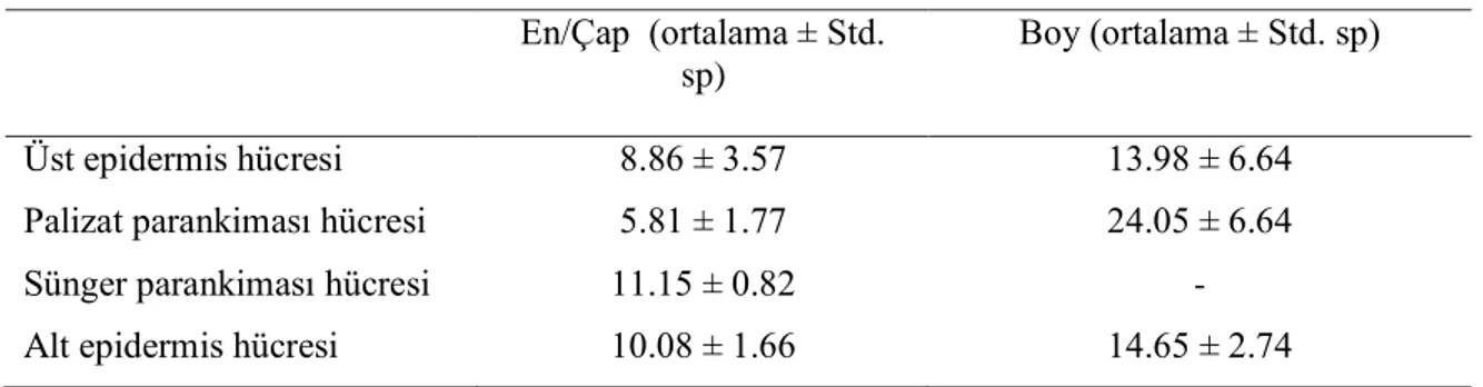
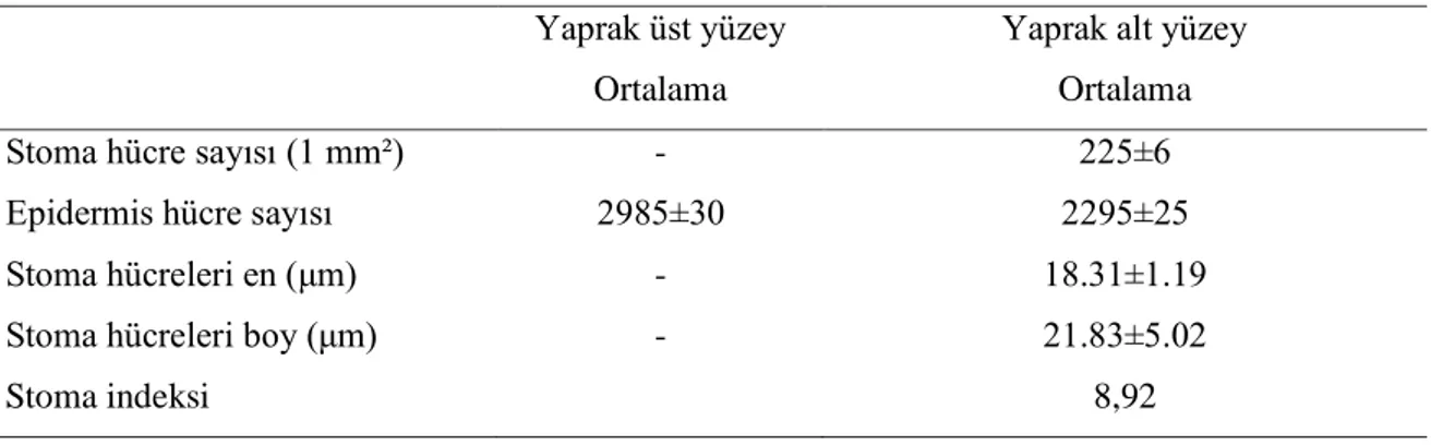
“Uzunmusa” Fındık Çeşidinin Yaprakları Üzerine Bir Araştırma………...65
Küresel Motor Çeşitleri………..70
Başlangıç Değer Problemi. Kirchhoff Formülü………...77
İnşaat Projelerinde Tespit Edilen Proje Risklerinin Proje Süresine Ve Maliyetine Etkisinin İncelenmesi……….93
Geciken Argümlü Adımlarla Ayrık Optimal Yönetim Olayının Araştırılması……….106
The Quantum Mechanical Rotation Operators Corresponding to Jz2 and J2 For All Spins………110
Makro-Sentetik Fiberli Betonların Mekanik Davranışının İncelenmesi………116
Simple Heliostat Design for Central Concentrated Solar Power System………...128
Artvin İlinin Madencilik Potansiyeli………...138
Farklı Sektörlere Ait Büyük Verinin Birliktelik Kuralları Yaklaşımıyla İncelenmesi………..155
The Quantum Mechanical Rotation Operators Corresponding to operators S + and S- For Spins 1/2 to 5/2………..165
Evaluation of Interfacial Maximum Stress Occurred Between Restorative Composite Resin Multilayer and Maxillary Tooth Surfaces By Using FEM………..171
Compressive Toughness Properties of Fly Ash Mortar Mixtures Containing Glass Powder as a Partial Replacement of Sand………...176
Determination of Surface Properties of Towel Samples in KES-FB4 Surface Friction & Geometric Roughness Test Measurement Device………182
Hidropolitik Açıdan Türkiye-Irak İlişkileri………...187
Ultrasonic Assisted Adsorption of Acid Red-1 Using Magnetic Zeolitic Tuff: Experimental Design Methodology……….205
Early Age Performance And Mechanical Characteristics of Concrete Which is Used in Service Buildings………...217
Using Frequency Selective Surface as a passive sensor in Structural Health Monitoring………227
Lyocell Liflerindeki Fibrilleşmenin Ultrasonik Yöntem Desteği İle Kontrolü………..233
The Effects of Biodiesels Produced from Edible and Non-Edible Plant Oil-Based Feedstocks on the Combustion Behaviors of Compression-Ignition Engines: A Review………245
Conditional Volatility Models in Financial Markets and Its
Application
Sakina I. BABASHOVA
Azerbaijan State University of Economics Turkish World of Economics Faculty, Department of Economics
E-mail: sbabashova@gmail.com
Abstract
Sudden and rapid changes in the economy leads to an increase in volatility. The fact that high volatility in financial markets brings along an increase in risk made it necessary to model it. Modeling volatility, which is accepted as a measure of risk, will benefit investors in their attitudes towards risk. The volatility of financial variables such as exchange rates, interest rates, and stock market indices is a measure of how far these variables deviate from their expected values.
ARCH-GARCH models, which are used in order to understand the dynamics of financial markets and to predict the changing volatility over time, have been expanded within the framework of some additional needs. Conditional volatility models are used extensively in modeling financial series. In general, ARCH models are models that relate the variance of error terms to the square of previous period error terms. The main feature of these models is that the variance of the error term in period t depends on the square of the error term in the period (t-1). In GARCH models, the error’s variance is not only associated with previous period errors but also with its own variance. The main feature of these models is that they allow varying variance of both autoregressive and moving average components. In order to model the volatility in financial time series, first it is necessary to test whether there is an ARCH effect in the model. If there is no ARCH effect in the model, the OLS estimation method can be used. However, if there is ARCH effect in error terms, the stage of estimating the variance model is started. Since the variance function is not linear, some iterative algorithms are used to maximize the likelihood function.
In this study, conditional volatility models that used in modeling the sudden and rapid changes in financial markets are discussed within the framework of other models that have been introduced in recent years. Then, conditional volatility models are applied on real data and obtained results are discussed.
Key Words: Volatility, ARCH-GARCH Models, Financial Markets
Introduction
In classical linear time series analysis, the variance of estimation errors is assumed constant, but it is seen that economic time series have fluctuation periods in most cases. Recent studies show that estimation with nonlinear time series models is more successful in explaining real life. Developments in nonlinear models day by day contribute to the expansion of application areas in the economics literature.
There are ups and downs in the economic conjuncture, and these dips are downsizing or stagnation, defined as a "recession regime", and downsides are a growth process, referred to as a "growth regime". The important point here is at what point the economy is in growth and contraction processes. Since classical linear time series techniques are not sufficient in this regard, nonlinear time series techniques are used in the analysis of these processes. The analysis tool is the reflection of developments in chaos theory in physics to statistics and economics. Here, the time series having a stochastic process is brought into a deterministic form.
Most of the economic variables consist of data in the form of time series. Time series analysis gives reliable results if many assumptions come true. One of these assumptions is the constant variance assumption. Therefore, it is important to determine and verify whether the error terms have a fixed variance.
If this problem is not solved, the coefficients have standard errors larger than necessary, while the constant variance assumption is not valid for most of the time series.
Choosing the comparative analysis of variance tests used in modeling nonlinear time series data as the subject of the study is important in terms of its currency. The main difference that distinguishes the study from the existing ones in the literature is the classification of variance tests; it is the comparison of five tests selected from different classes with different distributions based on the real data in terms of p value.
The aim of the study is to examine the theoretical structure of nonlinear time series models and to classify the heteroscedasticity tests used in these models. In addition, to determine the strengths and weaknesses of the tests during comparison, and to make interpretations on the usage areas of the tests based on real data.
Literature
Although the history of autoregressive conditional heteroscedasticity (ARCH) models is relatively short, the relevant literature has developed at a remarkable pace in this short history. Engle's original ARCH model (1982) and various extensions of this model have been applied to the economic and financial time series of many countries. Despite the awareness of the variance problem before the ARCH models were found, the problem was tried to be overcome by using processes not based on a specific model. Mandelbrot (1963) wanted to talk about the repeated estimates of variance over time, while Klien (1977) wanted to talk about the variance problem by using the five-period moving variances of the ten-period moving sample mean.
Financial time series have some general features. It has been observed that financial asset prices are generally not stable, asset returns are stable and do not show autocorrelation. Financial asset returns tend to be leptokurtic. The said return distributions are flatter than the normal distribution and have wider tails. This situation indicates that financial time series are more likely to change significantly than normal distribution. Another phenomenon frequently seen in financial asset returns is volatility clustering. It is seen that big changes follow big changes; small changes follow small changes in yield series. Essentially, the cases of thick tail and volatility clustering are interrelated. Finally, in the financial markets, market participants act differently against good and bad news. Bad news creates more volatility than good news. Hence, the direction of change in financial asset prices has an asymmetrical effect on volatility.
The ARCH model, proposed by Engle (1982), took its place in history as the first formal model to take into account the empirical findings in financial asset returns. The ARCH model is valuable not only because it takes into account some of the empirical findings in financial asset returns, but also because it finds application in different and multiple areas. For example, as used in asset pricing, it has also been used in measuring the maturity structure of interest rates, pricing options and modeling the risk premium. In the field of macroeconomics, the ARCH model has been successfully applied in forming the debt portfolios of developing countries, measuring inflation uncertainty, examining the relationship between exchange rate uncertainty and trade, investigating the effects of central bank interventions, and defining the relationship between macroeconomics and the stock market.
Bollerslev (1986) presented the Generalized Autoregressive Conditional Heteroscedasticity (GARCH) model by modeling conditional variance as an autoregressive moving average (ARMA) process unlike the ARCH model. The GARCH model is preferred over the ARCH model in terms of parameter conservation. Analyzing financial and economic time series data with ARCH and GARCH models has become widely used. Some of the studies on ARCH and GARCH models have been done by Bollerslev, Chai and Kroner (1992), Bollerslev, Engle and Nelson (1994), Bera and Hings (1993), Fountas, Karanasos and Mendoza (2004).
Engle et al. (1987) developed the Autoregressive Conditional Heteroscedasticity on Mean (ARCH-M) model by including conditional variance as an explanatory variable in the mean equation. The ARCH-M model is important in testing the relationship between uncertainty and return, which has an important place in finance theory.
Andersen (1996) developed the Mixture of Distribution Hypothesis and created a model by combining a stochastic volatility process with the GARCH method. He states that his model is useful in analyzing the economic factors behind the volatility cluster observed in financial returns.
Nelson (1991) developed the Exponential GARCH (EGARCH) model to explain the asymmetric volatility structure observed in financial markets. In this model, the conditional variance may vary depending
not only on the magnitude of the shock, but also on its sign. Another important model that takes into account the asymmetric volatility structure is the Threshold ARCH (TARCH) model proposed by Zakoian (1994).
The univariate ARCH / GARCH approach is criticized as it does not take into account the time dependence between conditional variance and covariance between various markets and assets. To explain the time dependence in question, Bollerslev et al. (1988) extended univariate ARCH / GARCH models to multivariate models under the name of VEC parameterization. The VEC-GARCH model has problems in terms of applicability since it requires a large number of parameter estimates and the positive definition of the covariance matrix cannot always be achieved.
The VEC-GARCH model can be transformed into a model in which the positive definition of the covariance matrix is provided. This transformed model is known as the BEKK-GARCH model as defined in Engle and Kroner (1995).
Engle et al. (1990) put forward the Factor GARCH (F-GARCH) model in which the conditional correlation matrix is generated by fundamental factors. Bollerslev (1990) proposed the Constant Conditional Correlation GARCH (CCC-GARCH) model in which the number of parameters to be predicted is considerably reduced and the estimation process is quite simplified when conditional correlations are constant.
Whether or not conditional correlations are constant is not always a satisfactory condition as it is a purely empirical problem. For cases where conditional correlations are not constant, Tse and Tsui (2000) and Engle (2001) created two separate dynamic conditional correlations (DCC) parameterizations. In addition, Tse (2000) and Engle and Sheppard (2001) developed two separate fixed conditional correlation tests to test whether the conditional correlations are constant.
Threshold Autoregressive (TAR) models have become common in econometrics literature in the last two decades. TAR models were first presented in the studies of Tong (1978), Tong and Lim (1980) and Tong (1983). The main reason for the popularity of models is the ease of application of these techniques and the interpretation of their results, and the prediction is relatively simple. Another important feature of TAR models is that even in the presence of a small number of regimes, a nonlinear cascade dependent structure can be explained by the threshold pipeline dependency.
The GARCH model and its various variations have been very useful in measuring the volatility in time series. However, when there are one or more breaks in the variance of the series, it has been revealed that the volatility measured by ARCH-GARCH models is higher than it is. Lamoureux and Lastrapes (1990) raised the question of whether the calculated volatility will be greater due to deterministic structural breaks in the series. For this purpose, considering the 30 exchange rate series, they revealed that when regime shifts are directly included in the ARCH / GARCH model, the variance persistence obtained in the GARCH model significantly decreases. Since there was no method to find the breakpoints in variance, they divided the sampling period into equally spaced, non-overlapping intervals as a solution, and tested how sudden changes in variance affect the parameters of the predicted models.
Aggarwal (1999) used the ICSS (Iterative Cumulative Sum of Squares) algorithm to detect volatility changes in stock returns and found that if these breaks are ignored, volatility persistence will be higher than it is. Fernandez (2005), in order to reveal the impact of the Asian crisis and September 11 attacks on international financial markets, using the ICSS algorithm, determined the variance breaking and compared the results with the Wavelets method. He revealed that the breaks he found with both methods caused decreases in volatility when taken into consideration.
Since ARCH (GARCH) models are an iterative estimation process, it can be decided by testing whether the model includes autoregressive conditional heteroscedasticity (ARCH) effect or not. The special test developed to determine whether ARCH effects exist in time series was developed by Engle (1982). This test, also known as the ARCH LM test, is a Lagrange Multiplier (LM) test that investigates whether the model has ARCH effects in error terms. The reason for the investigation of ARCH effects, which is a special form of heteroscedasticity, is that the current error term, which is observed in many financial time series and, if neglected, reduces the effectiveness of the estimates, and the fact that the recent error terms are more closely related than the error terms of the previous periods should be taken into account .
There are many other statistical methods used in determining the variance problem in the literature: White general variance test (1995), Park test (1964), Glejser test (1969), Goldfeld-Quandt test (1972), Spearman
rank correlation test (1904), Breusch -Pagan-Godfrey test (1979), Ramsey's Reset test (1969), BDS linearity test developed by Brock, Dechert and Scheinkman (1987), Bartlett's Equal Variance test (1937).
Methodology
Autoregressive Conditional Heteroscedasticity (ARCH) Model
Although the heteroscedasticity problem is generally known as a problem that occurs in cross-section data, it has been observed that the error variance can change over time in econometric models that aim to predict financial time series such as exchange rate, interest rate and stock price. In general, it is assumed that the error variance in time series models does not change over time. Therefore, it is important to determine and verify whether the error terms have a fixed variance. If this problem exists and cannot be solved, the coefficients will have standard errors larger than necessary (Enders, 2004: 82-84).
The econometric approach assumes that autocorrelation is a time series and variance is a cross-sectional data problem. In this case, according to traditional techniques, it is accepted that the variance of the error term is constant, that is, it does not change over time. However, it is seen that the time series of many macroeconomic and financial variables generally exhibit wide variability, and in time series of such macroeconomic variables, the assumption that the variance of errors is constant over periods is not appropriate. In fact, in such cases, some kind of autocorrelation is encountered in predictive variances. However, in the traditional econometric approach, it is mentioned that changing variance will occur mostly in models using cross-sectional data, while time series data are used in models with constant variance (Brockwell, Davis, 1991: 103).
With Engle's article published in 1982 using UK inflation data, an important step was taken in estimating conditionally heteroscedasticity models. Engle determined this conditional variance as a function of the squares of the error terms in cases where the conditional variance is time dependent while the unconditional variance is constant (Engle, 1982: 994). In order to stabilize the series in which the variance is not constant, the most popular nonlinear models that can be applied without transforming them with exponential transformation techniques such as Box-Cox transformation are ARCH (Autoregressive Conditional Heteroscedasticity) models in the literature.
Contrary to the common assumption in the literature, it has been proved by Engle that the variance of error terms in time series models is not constant by analyzing some macroeconomic data. Engle found that large and small estimation errors occur in clusters in inflation models, and as a result showed that the variance of estimation errors depends on the size of the previous period's error terms. He pointed out that autocorrelation, which is encountered in time series data and shows itself especially in predictions, should be modeled with a technique called ARCH (Engle, 1982: 987-1006).
The ARCH model leaves the constant variance assumption in traditional time series models, allowing the variance of the error term to change as a function of the squares of the previous period error terms. As one of the ways of modeling the volatility observed in time series, defining an independent variable related to volatility and estimating the volatility through this variable comes to the fore. As a simple example reflecting the case in which volatility is modeled by defining it as an independent variable,
t t
t x
y 1
1 (1) In this equation, xt is defined as an independent variable, while
t1 is a pure error term with 2 variance. If x takes a constant value regardless of time, the {yt} series becomes a white noise process with constant variance. However, the conditional variance of yt+1,
2 21 t t
t x x
y
Var (2) is not independent of the actual value of xt. In this case, the larger the xt, the greater the conditional variance of yt+1. If the consecutive values of the {xt} series are positively intrinsically correlated, the {yt} series will also be positively intrinsically correlated. In this way, the {xt} series will help explain the volatility in the {yt} series. However, one drawback of this approach is that it assumes a specific cause for the variance. It is not always possible to choose one among many candidates that seem reasonable and to relate the volatility in the relevant variable only to the preferred independent variable.
Engle (1982) showed that it is possible to model the mean and variance of any series simultaneously in order to eliminate this drawback. To reach the ARCH model, a stationary autoregressive model is predicted as t t o t y y
1 1
(3) In this case, the conditional estimate of yt+1,t t
t y y
E ( 1)
0
1 (4) If we use this conditional mean to estimate yt+1, the prediction error variance is,
2 2 1 2 1 0 1
t t t t ty
y
E
E
(5) On the other hand, the unconditional estimation and variance of yt+1 are, respectively,
yt1
0
1
1
E (6)
2 1 2 2 2 1 2 1 1 1 2 1 0 1 1 ... 1 t t t t E y E (7)As you can see, unconditional estimation has a greater variance than conditional estimation. Therefore, conditional estimation has smaller variance and becomes preferable in this context, since it takes into account past realizations known with the current period.
Similarly, if the variance of the {εt} series is not constant, ARMA model can be used to estimate the continuous movement in a certain direction in the variance. As an example of this situation, assuming that
t
is a residual series of the model
t t
t
y
y
0
1 1
, (8) so the conditional variance of yt+1 is
2 1 2 1 0 1 1 t t t t t t t y E y y E y Var (9) At this point, it is necessary to establish a structure where the conditional variance in equation (9) is not constant and changes over time. Modeling the conditional variance as an AR(q) process using the squares of estimated residuals is shown below. The model is the squared of estimated residuals, where νt is a white noise process, t q t q t t t2
0
1
21
2
22
...
2
v
. (10)If the parameters other than the constant value in the model were zero, the estimated variance would be equal to the constant value α0. In other cases, the conditional variance of yt will be determined within the framework of the autoregressive process in equation (1.10). In this framework, the conditional variance one term next is estimated using the autoregressive process,
2 1 2 1 2 2 1 0 2 1 t t
...
q t q t tE
(11) For this reason, equation (10) is called the ARCH (q) model.Defining vt as a multiplicative error term instead of linear definition in Equation (10) creates a structure that can be examined more easily. Engle (1982) proposed the simple model as an example of multiplicative conditionally variance type models,
2 1 1 0 t t t v
(12) Here, vt is defined as a white noise process whose variance is equal to one, and vt and
t1 are independent of each other. In addition, they take constant values of α0 and α1 under the constraints of α0>0 and 0<α1<1.When the properties of the
t series are examined, it is not difficult to show that each of the elements in the
t series has a zero mean and is intrinsically unrelated, since vt is a pure error term and is independent of
t1.Since Evt 0, unconditional expectation of
t is,
0 1 21
1/2
0 1 21
1/2 0 t t t t t E v Ev E E (13)Similarly, the unconditional variance of
t is calculated as
2
1 1 0 2 2 1 1 0 2 t t t t t Ev Ev E E
(14) Here, since the variance of vt is equal to one and the unconditional variance of
t is the same as the unconditional variance of
t1, the unconditional variance is calculated as,) 1 ( 1 0 2 t E (15) Therefore, the error process does not affect the unconditional mean and variance and they take constant values.
The conditional variance of
t ceases to be a fixed value and becomes dependent on its value that wasrealized a period ago. Since the variance of vt is equal to one, the conditional variance of
t is calculated as
2 1 1 0 2 1 2,
,...
)
(
t
E
t t t
th
(16) The conditional variance in Equation (16) is a first order autoregressive process. In order to prevent conditional variance from taking negative values, it is necessary to limit the coefficients α0 and α1. Accordingly, the coefficients α0 and α1 must be positive. In addition, in order to ensure the stability of the autoregressive process, it is necessary to limit the α1 coefficient to ensure inequality011.As a result, there is an error structure in the ARCH model in which the conditional and unconditional mean equals zero. In addition, although the series
t is not intrinsically related, the error terms are notindependent from each other because they are related through their second moments. Conditional variance itself is an autoregressive process that consists of conditional heteroscedastic errors. The greater the error term occurred a period ago from zero as the absolute value, the greater the conditional variance of
t.Weaknesses of the ARCH Model
Although the ARCH model captures some empirical findings seen in asset returns and proposes a parametric structure for estimating volatility in this framework, it also has some important weaknesses (Tsay, 1986: 112). These weaknesses are listed as follows:
1. Since the shocks of the previous period are included in the model by being squared, it is assumed that positive and negative shocks have the same effect on volatility. However, it is known that financial asset prices can respond asymmetrically to negative and positive shocks in real life.
2. The coefficients in the ARCH model are subject to very strict constraints.
3. The ARCH model does not make any new contribution to understanding the source of changes in financial time series; it only suggests a mechanical way to determine how conditional variance behaves.
4. Since ARCH models react slowly to large shocks to financial returns, they can predict the volatility of financial time series more than they are.
Definition of Heteroscedasticity Problem
One of the most important assumptions of the Least Squares (OLS) technique in Classical Linear
Model Analysis is the constant variance assumption. The OLS technique assumes that the variance
of the unit values of the dependent variable will remain constant while the unit values of the
independent variables change, and this assumption is called homoscedasticity in the statistics
literature (Gujarati, 1995: 73; Orhunbilge, 2000: 69; Tarı, 2006: 101). In other words, the error term
variance is not affected by the changes in the independent variables and remains the same. The
homoscedasticity assumption can be represented as follows:
N N N N i i i i I u u E N i u E u Var X u Var 2 2 2 2 2 2 2 0 0 0 0 0 0 1 0 0 0 1 0 0 0 1 ..., , 2 , 1 (17)
The assumption that the variance of the error term ui is equal for each explanatory variable Xi is expressed as follows:
2 i i i iX
E
u
E
u
u
Var
(18) Since
u
i
0
E
(19)
2
2 i i iX
E
u
u
Var
(20) It is also Var
ui VarYi 2. The meaning of this assumption is as follows: For each value of Xi, the conditional variance of the error term ui is a certain constant and is equal to 2. On the other hand
2i i X
Y
Var . Homoscedasticity is shown in Figure 1 below. In this way, it is seen that the conditional variance of Y is constant for the simple linear regression model with two variables.
Figure 1. The Case of Homoscedastic Error Term
Source: Gujarati, 1999:68
Despite the afore mentioned facts, in Figure 2 the values of X increase from left to right (X1, X2,...,Xi) and it is observed that mass variance of Y increase and curves are gradually spread and disperse in a wider area. This situation is called heteroscedasticity.
Figure 2. The Case of Heteroscedastic Error Term
Source: Gujarati, 1999:69
The difference in the variance of the error term indicates the undesired situation in regression analysis. In this case, the variance of the errors of the regression model is not constant, but may change by showing an increasing, decreasing or both increasing and decreasing distribution:
u
X
Var
u
E
u
f
X
i
n
Var
i i
i
i2
i2
i,
1
,
2
,
...,
(21) The heteroscedasticity problem can be represented by matrix as follows:
u
u
2
ve
1
E
(22) is the matrix, the non-diagonal elements are zero, but the variances on the diagonal are different. The Results of Heteroscedasticity
In cases where there is heteroscedasticity, the estimation results obtained by the OLS method preserve their non-deviating, consistent and linear properties, but they lose the feature of being efficient and the best estimator, that is, being the least variance to the class of estimators without linear deviation. In case of heteroscedasticity, parameter estimates are no longer the best and their variances are not minimal. In this case, standard errors calculated for model parameters do not give correct results. Therefore, test’s results and confidence intervals are misleading. If the variance of the error terms is gradually increasing, the estimates found by the OLS method may cause a lower variance and standard error than necessary. Therefore, t statistics will be higher than they should be, and confidence intervals will be narrower. As a result, it will be seen that there is more reliance on the forecast results than it should be. Conversely, if the variance of the error terms is gradually decreasing, the parameter estimates obtained by the OLS method may cause a larger variance and standard error than necessary.
Inaccurate estimation of the variances of the parameter estimators leads to inaccurate range estimates, t and F tests. After all, the statistics obtained will be less reliable than necessary.
How to Detect Heteroscedasticity?
Since heteroscedasticity can be a serious problem, the researcher has to know whether it exists or not. How we can answer the questions about whether there is heteroscedasticity in a particular situation or whether it exists is explained below.
As with multicollinearity, there are no precise rules for understanding the existence of heteroscedasticity, there are some finger calculation rules. Nevertheless, this situation is unavoidable, because i2 can only be
known if we know the entire Y population corresponding to the selected X's. But in most economic studies, such data are the exception rather than the rule. In economics research, there is often a single sample value Y for a given value of X. It is impossible to know i2from a single Y observation.
With the above warning in mind, a few formal and non-formal methods used in detecting heteroscedasticity are mentioned below. Most of these methods are based on examining the error terms of the model.
Tests for Determining ARCH and GARCH Effects
Tests to determine the effects of ARCH and GARCH are based on the assumption that the residuals' own past values lead to heteroscedasticity. This means the sequential dependence (autocorrelation) in the variance of the error term. Autocorrelation is a problem mostly encountered in time series and heteroscedasticity is
mostly encountered in cross-section data. However, forecasting errors in financial time series such as stock prices, exchange rates, inflation rates can be small in some periods and large in some periods, which shows that the variance of the error term is not constant but varies from period to period.
Before applying the ARCH method, it is necessary to test whether the ARCH effect is present or not for the series related to a variable. When the ARCH effect is ignored in time series, the effectiveness of estimates decreases (Engle, 1995: 201).
The error terms are not correlated in the series in which the ARCH structure is observed. However, the variance depends on past values. Therefore, meaningful DW statistics resulting from the ARCH effect are obtained. Durbin-h test is used in a first order autoregressive structure. It is appropriate to use the Lagrange Multiplier (LM) test, which is a more general test in higher order autoregressive structures (Maddala, 1992: 152).
The two most important tests suggested in the literature to test the presence of ARCH effect are Engle's (1982) ARCH LM test (Engle, 1982: 987-1006) and McLeod and Li's (1983) Q test (McLeod, Li, 1983: 269- 273). The ARCH LM test is the most preferred test in detecting the ARCH effect because it is easy to derive and gives good results. The purpose of ARCH LM testing on residuals is to test the presence of heteroscedastic errors in the model. Standard errors will be downwardly deviated along with the parameters in the model (Cromwell, Labys, Terraza, 1994: 73).
The Comparison of Heteroscedasticity Tests Based On Real Data
In this section of the study, numerous international A typed numerical data were used in the period before 30.12.2010 taking into consideration the increase in the net assets. While analyzing these funds, special attention was given to developing countries from America, Europe, Asia and other continents and among them, 11 A type stock funds were given attention in the study. Selected international funds are listed in Table 1.
Selected 11 funds consist of five different categories. Three of them are Diversified Emerging Markets whereas five are from Latin America. One of these 11 funds is from Pacific-Asia countries outside Japan. The nest two are from Turkey market and Europe.
Table 1: International A typed Mutual Funds FUN
D CODE
FUND NAME FUND CATEGORİES
1 DPC
AX Dreyfus Greater China A
Pacific-Asia countries outside Japan
2 FAF Finansbank A.Ş. A Turkey
3 FLA
TX Fidelity Latin America Latin America
4 FLT
AX
Fidelity Advisor Latin
America A Latin America
5 GTD
DX
Invesco Developing Markets
A Diversified Emerging Markets
6 LET
RX ING Russia A Europe
7 MDL
TX BlackRock Latin America A Latin America
8 PRL
AX T.Rowe Price Latin America Latin America
9 PTE
MX
Forward Emerging Markets
Instl Diversified Emerging Markets 1
0
QFF
OX Quant Emerging Markets Ord Diversified Emerging Markets 1
1
SLA
FX DWS Latin Amerika Equity S Latin America Descriptive Statistics and Stability Tests of Mutual Funds
For the international funds that have been mentioned in the study, 1510 observations covering the period between 01.01.2004 – 01.01.2010 were used. 1510 observation values are the price funds announce daily. The International funds’ series are shown in Figure 3.
With the purpose of getting the chance for the return series, first degree logarithmic differences of the prices of the funds announced daily between 01.01.2004-01.01.2010 were taken1. Descriptive statistics of 11
international A typed stock funds and the results of normality tests are shown in Table 2.
Figure 3. Series for International Funds. (2004-2009)
Table 2: Descriptive Statistics and Stability Test Results of Mutual Funds
Fund Code Ave. Med. Max Min S.D. Skewness Kurtosis AsymptoticTest N orma-lity Test RDPCAX 0,0006 0,001 0,09 -0,136 0,018 -0,662 10,12 3279,48 7 05 RFLATX 0,0009 0,002 0,208 -0,176 0,023 -0,249 13,63 7084,90 1 548 RFLTAX 0,0009 0,002 0,206 -0,176 0,023 -0,260 13,67 7127,82 1 547 RGTDDX 0,0006 0,001 0,096 -0,095 0,014 -0,581 9,28 2552,63 6 60 RLETRX 0,0004 0,002 0,188 -0,319 0,027 -1,671 24,89 30627,8 1668 RMDLTX 0,001 0,002 0,225 -0,189 0,024 -0,376 15,46 9740,39 1 821 RPRLAX 0,0008 0,002 0,220 -0,163 0,023 -0,249 14,32 8019,08 1 788 RPTEMX 0,0003 0,002 0,132 -0,127 0, 018 -0,666 13,36 682 2,50 1 557 RQFFOX 0,0005 0,002 0,114 -0,106 0, 016 -0,538 1 2,01 514 1,60 1 096,4 RSLAFX 0,0006 0,0023 0,213 -0,184 0, 024 -0,550 14,21 7931,59 1 480,9 RFAF 0 ,001 0,0008 0 ,095 -0,098 0,015 -0,132 4,80 1459 ,30 574,3
The critical value with 2 degree of freedom of
2table on the 5% confidence plane is 5.99 Summaries about the descriptive statistics on the base of Table 2 are as following;1) LETRX fund has high volatility level among the international funds. (S.D.=0,027).
1 1 ln t t t P P r 10 20 30 40 50 60 70 2004 2005 2006 2007 2008 2009 DPCAX 0 20 40 60 80 2004 2005 2006 2007 2008 2009 FLATX 10 20 30 40 50 60 70 2004 2005 2006 2007 2008 2009 FLTAX 10 15 20 25 30 35 40 2004 2005 2006 2007 2008 2009 GTDDX 0 20 40 60 80 100 2004 2005 2006 2007 2008 2009 LETRX 0 20 40 60 80 100 2004 2005 2006 2007 2008 2009 MDLTX 0 20 40 60 80 2004 2005 2006 2007 2008 2009 PRLAX 8 12 16 20 24 28 32 36 2004 2005 2006 2007 2008 2009 PTEMX 8 12 16 20 24 28 32 36 2004 2005 2006 2007 2008 2009 QFFOX 20 40 60 80 100 2004 2005 2006 2007 2008 2009 SLAFX .00 .02 .04 .06 .08 .10 2004 2005 2006 2007 2008 2009 FAF
2) On the basis of the differences between the Maximum and Minimum values, LETRX and MDLTX funds are the funds with the highest volatility.
3) In terms of the Skewness, all international funds have negative values. This values indicate that fund return series are skewed to the left. LETRX fund has the highest asymmetric structure.
4) When Kurtosis values are investigated it is observed that all international funds return series have fat tail structure. LETRX has the highest kurtosis value. When asymptotic test results are compared with value with 2 degree of freedom of
2table on the 5% confidence (5.99) it became clear that as all international funds have the value higher than 5.99, they are not normally distributed. This asymmetric structure of the international funds is revealed with clustering of volatility and extreme fluctuations in several periods. Return series for international funds are shown in Figure 4.Figure 4. International Funds Return Series (2004-2010)
As it is clear from Figure 4, in all international funds there was increase in volatility in the 2008s. The increases were for short term in 2006 but in 2008 they were for a long period. Especially in 2004-2010 period, the wild fluctuation was observed in FAF fund being different from other funds.
The Application of Heteroscedasticity Tests on Real Data
The results of stationary test show that return series of international funds are not stationary and they comprise asymmetric effects. As the financial asset return series lose normal distribution feature with the impact of shocks, the models should consider the volatility.
In the application section, normality test with the purpose of determining the conditional heteroscedasticity was made and return series’ was determined. Then working on each return series correlograms were examined and the information about autoregressive structure (AR) was obtained.
Several AR structures were tested for the return series and it was decided to choose models that suggest the lowest AIC and Schwarz criterion values. Then, errors given by the main models were studied, and Park, Glejser, BG LM, White and ARCH LM tests were applied and test statistics were obtained (see Table 3).
The comparison of Park, Glejser, BG LM, White and ARCH LM heteroscedasticity tests that were applied on the international funds were made in terms of p value. Here, the lowest probability value is given and H0 hypothesis for each observed test statistics is accepted and because of comparison of this probability
value with
significance level it is decided whether to accept or reject H0 hypothesis.Generally:
- When P value is below 1%, there is a very strong evidence that in this situation, alternative hypothesis is right;
- When P value is between %1 and %5 there is a strong evidence that in this situation, alternative hypothesis is right; -.15 -.10 -.05 .00 .05 .10 2004 2005 2006 2007 2008 2009 RDPCAX -.2 -.1 .0 .1 .2 .3 2004 2005 2006 2007 2008 2009 RFLATX -.2 -.1 .0 .1 .2 .3 2004 2005 2006 2007 2008 2009 RFLTAX -.10 -.05 .00 .05 .10 2004 2005 2006 2007 2008 2009 RGTDDX -.4 -.3 -.2 -.1 .0 .1 .2 2004 2005 2006 2007 2008 2009 RLETRX -.2 -.1 .0 .1 .2 .3 2004 2005 2006 2007 2008 2009 RMDLTX -.2 -.1 .0 .1 .2 .3 2004 2005 2006 2007 2008 2009 RPRLAX -.15 -.10 -.05 .00 .05 .10 .15 2004 2005 2006 2007 2008 2009 RPTEMX -.12 -.08 -.04 .00 .04 .08 .12 2004 2005 2006 2007 2008 2009 RQFFOX -.2 -.1 .0 .1 .2 .3 2004 2005 2006 2007 2008 2009 RSLAFX -.10 -.05 .00 .05 .10 2004 2005 2006 2007 2008 2009 RFAF
- When P value is between %5 and %10 there is a weak evidence that in this situation, alternative hypothesis is right;
As p0,01 is found for the Park and Glejser tests that are applied for the international return fund series, H0 hypothesis (H0: absence of heteroscedasticity) is strongly rejected; very strong decision can be made
about the correctness of alternative hypothesis (Ha: presence of heteroscedasticity). As the BG LM test
statistic is p < 0,05 for 8 series (besides MDLTX, PRLAX, SLAFT), H0 hypothesis is strongly rejected and it
Table 3: Heteroscedasticity Tests Results for International Funds
FUND CODE
Park Glejser BG LM White ARCH LM
tist N*R2 Pvalue tist N*R2 Pvalue tist N*R2 Pvalue tist N*R2 Pvalue tist N*R2 Pvalue
LETRX 2,98 8,88 0,0029 3,08 9,47 0,0021 3,09 11,82 0,0027 4,02 16,03 0,000 5,48 29,43 0,000 MDLTX 2,22 4,92 0,0264 2,42 5,87 0,0154 1,75 3,15 0,206 3,27 10,68 0,001 5,17 26,34 0,000 PRLAX 2,79 7,75 0,0054 3,21 10,26 0,014 2,37 7,69 0,213 3,52 12,35 0,000 5,34 28,02 0,000 PTEMX 2,68 7,14 0,0075 3,35 11,16 0,0008 2,37 6,46 0,0396 5,8 36,81 0,000 4,93 23,95 0,000 SLAFT 2,38 5,66 0,0174 2,52 6,36 0,0116 1,88 4,94 0,1756 2,83 8,01 0,004 5,04 24,99 0,000 FLTAX 2,68 7,19 0,0073 3,16 9,93 0,0016 2,55 6,52 0,0107 3,81 14,42 0,000 5,59 30,67 0,000 QFFOX 3,27 10,63 0,0011 3,31 10,92 0,011 2,03 4,11 0,0425 4,88 26,52 0,000 7,6 55,78 0,000 FLATX 2,85 8,1 0,0043 3,26 10,54 0,0012 2,08 7,99 0,0462 3,78 14,24 0,000 5,63 31,14 0,000 DPCAX 2,42 5,85 0,0156 3,36 11,26 0,0008 3,51 12,79 0,0051 4,59 30,81 0,000 3,96 15,54 0,000 GTDDX 2,42 5,85 0,0156 2,86 8,14 0,0043 3,49 13,03 0,0046 3,57 12,64 0,00037 6,07 35,97 0,000 FAF 3,02 9,099 0,0026 3,1 9,572 0,002 2,13 4,558 0,0328 4,45 22,632 0,000 6,08 36,17 0,000
When the probability of p rejecting values for White and ARCH LM test statistics are examined, for 11 international investment fund series p0,01 was found. As it was in the results of Park and Glejser tests, H0
hypothesis is strongly rejected because of application of White and ARCH LM tests. In this case, decisions can be made about the correctness of alternative hypothesis. However, when compared with Park and Glejser tests heteroscedasticity tests, p values of White and ARCH LM test statistics equal to lower values. For this reason, White and ARCH LM tests seem more advantageous than the others do.
Conclusion
White and ARCH LM heteroscedasticity tests were the strongest tests because of study; they had the lowest p value in the application section.
Taking into consideration the problems being encountered during the study and the results, I am of the opinion that if the following subjects are examined carefully, they will be very useful for the future investigator in this topic.
1) The same methodology can be used for the other nonlinear models except the comparison of variable variances that have been investigated in this study.
2) With the purpose of obtaining of nonlinear time series, full stationary nonlinear time series ARCH(1) and full stationary nonlinear time series ARCH(2) process’ were taken into consideration. This study can also be repeated for high-level nonlinear models.
3) The same methodology can be used for other heteroscedasticity tests.
References
Bates, D., Watts, D. (1988). Nonlinear Regression Analysis and It’s Applications. USA: John Wiley& Sons. Bollerslev, T., Engle, R. and Nelson, D. (1994). ARCH Models. Handbook of Econometrics.
Box, G., Jenkins, G., and Reinsel, G. (1994). Time Series Analysis: Forecasting and Control. 3rd edition. New Jersey: Prentice-Hall.
Breusch, T., and Pagan A. (1978). A Simple Test for Heteroscedasticity and Random Coefficient Variation.
Econometrica, 46:1287-1294.
Brooks, C. (2002). Introductory Econometrics for Finance. Cambridge: Cambridge University.
Campbell, J., Andrew W. and MacKinlay A. (1997). The Econometrics of Financial Markets. Princeteon: Princeton University.
Chatfield, C. (1989). The Analysis of Time Series an Introduction, New York: Chapman and Hall. Engle, R. (1995). ARCH Selected Readings. New York: Oxford University Pres.
Engle, R. (1982). Autoregressive Conditional Heteroscedasticity with Estimates of the Variance of United Kingdom Inflation. Econometrica, 50(4):987-1006.
Gallant, A. (1987). Nonlinear Statistical Models, USA: John Wiley & Sons.
Glejser, H. (1969). A New Test for Heteroscedasticity. Journal of American Statistical Association, 64:316-325.
Godfrey, L. (1978). Testing Against General Autoregressive and Moving Average Error Models When the Regressors Include Lagged Dependent Variables. Econometrica, 46:1293–1301.
Gourieroux, C. (1997). ARCH Models and Financial Applications, New York: Springer-Verlag New York. Granger, C. and Terasvirta, T. (1993). Modelling nonlinear economic relationships. New York: Oxford
University Press.
Hamilton, J. (1994). Time Series Analysis. New Jersey: Princeton University Press.
Murphy, K. and Myors B. (1998). Statistical Power Analysis. A Simple and General Model for Traditional
and Modern Hypothesis Tests. London, UK: Lawrence Erlbaum Assoc.
Park, H. (2008). Hypothesis Testing and Statistical Power of a Test. Working Paper. Indiana University: The University Information Technology Services (UITS) Center for Statistical and Mathematical Computing. http://www.indiana.edu/~statmath/stat/all/power/index.html
Park, R. (1964). Estimation with Heteroscedastic Error Terms. Econometrica, 34(4):888.
Pindyck, R. and Rubinfeld, D. (1991). Econometric Model and Econometric Forecast, 3rd Ed. Irwin: McGraw-Hill.
Priestley, M. (1988). Non-linear and Non-Stationary Time Series Analysis. New York: Academic Press. Resnick, S. and van Den Berg, E. (2001). A test for non-linearity of time series with infinite variance.
Extremes, 3, 145–172.
Stock, H. and Watson, W. (2020). Introduction to Econometrics, Global Edition, 4th Edition. Person
Stuart, A. and Ord, J. (1994). Kendall's Advanced Theory of Statistics. Volume 1: Distribution Theory. 6th edition. New York: John Wiley & Sons Inc.
Terasvirta, T. (2009). An Introduction to Univariate GARCH Models. Handbook of Financial Time Series. New York: Springer.
Terasvirta, T., Tjostheim, D. and Granger, C. (1994). Aspects of Modelling Nonlinear Time Series. Handbook of Econometrics, Oxford: Elseiver.
Tsay, R. (2002). Analysis of Financial Time Series. New York: John Wiley & Sons.
81 İldeki 2010-2013 Yıllarına Ait Trafik Cezalarının Karşılaştırılması
Ebru Arıkan Öztürk
Gazi Üniversitesi Trafik Planlaması ve Uygulaması ABD
eozturk@gazi.edu.tr
Özet
Günümüzde kentlerin en önemli sorunlarından biri de trafik güvenliğidir. Trafik denetimleri, trafik güvenliğinin artırılması için uygulanacak pek çok stratejiyle birlikte, temel bir strateji olarak karşımıza çıkar. Türkiye’de trafik denetleme görevi Trafik Polisi, Jandarma Trafik Birimleri ve Fahri Trafik Müfettişleri tarafından (FTM) gerçekleştirilmektedir. Çalışmanın amacı trafik cezalarının trafik güvenliğine etkisini ortaya koymaktır. Bu doğrultuda öncelikle Türkiye’deki 81 ilin ölümlü kaza verileri ortaya konulmuş, daha sonra 2010-2013 yıllarını kapsayan 4 yıllık süreçte Polis ve FTM tarafından sürücülere yazılan ceza miktarları il düzeyinde karşılaştırmalı olarak incelenmiş, yazılan cezalar ile trafik kazalarındaki ölüm miktarı değişimleri bir arada değerlendirilerek trafik cezaları-trafik güvenliği ilişkisi ortaya konulmuştur. Polis ve FTM’nin sürücülere yönelik denetleme faaliyetlerinin trafik güvenliğine olumlu katkı sağladığı sonucuna varılmıştır.
Anahtar Kelimeler: Fahri Trafik Müfettişi, Trafik güvenliği, Denetleme.
Abstract
Traffic safety is one of the most important problems of cities today. Traffic enforcement constitutes a main strategy in addition to several other strategies to be implemented for increasing traffic safety. In Turkey, traffic inspections are carried out by Traffic Police, Gendarmery Traffic Units and Voluntary Traffic Inspectors (VTI). The purpose of this study was to reveal the effects of traffic fines on traffic safety. For this purpose, the fatal accident data of the 81 provinces in Turkey were presented first, and the amounts of fines that were issued in the 4-year period of 2010-2013 by the Police and VTI on the provincial level were comparatively analyzed, The relationship between traffic fines and traffic safety were presented by assessing the fines that were issued and the changes in the fatality rates together. It was concluded that the inspection activities towards drivers by the Police and VTI provided positive contributions on traffic safety.
Keywords: Voluntary Traffic Inspector, Traffic safety, Enforcement
1. Giriş
Trafik kazalarında meydana gelen ölüm, yaralanma ve maddi kayıplar tüm dünyada olduğu gibi Türkiye’de de büyük önem taşıyan bir halk sağlığı sorunudur. Dünya Sağlık Örgütü’ne göre her yıl 1,35 milyon kişi trafik kazası nedeniyle hayatını kaybetmekte, onlarca milyondan fazla kişi de yaralanmakta ya da sakat kalmaktadır (DSÖ, 2018). Dünyadaki ilk on ölüm nedeni sıralamasında yol trafik kazaları 8. sıradadır ve gerekli önlemler alınmazsa 2030 yılına kadar 5. sıraya yükseleceği öngörülmektedir. (DSÖ, 2013). Ayrıca trafik kazaları ile miktarı ciddi boyutlara ulaşan toplumsal ve ekonomik kayıplar oluşmaktadır.
2017 yılında Türkiye’de meydana gelen trafik kazalarında 3534’ü kaza yerinde 3893’ü kaza sonrası olmak üzere toplam 7,427 kişi hayatını kaybetmiş, 300,383 kişi de yaralanmıştır. Ölü sayıları 2015 yılına kadar sadece kaza yerinde tespit edilen ölümleri kapsarken, 2015 yılından itibaren trafik kazasında yaralanıp sağlık kuruluşuna sevk edilenlerden kaza nedeniyle 30 gün içinde ölenleri de kapsamaktadır (EGM, 2017). 2017 yılı trafik kaza istatistikleri incelendiğinde meydana gelen kazaların; %90,3’ünün sürücü, %8,3’ünün yaya ve %0,4’ünün de yolcu kusurları olmak üzere toplam %99 oranla yol kullanıcı kusurlarından kaynaklandığı anlaşılmaktadır (KGM, 2017). Bu yüksek oran, trafik kazası tespit tutanağında yol ve araçla ilgili kusurların net olarak belirlenememesi nedeniyle istatistiklere böyle yansımış olsa da, meydana gelen ölümlü kazalarda sürücü hata ve ihlalleri önemli pay sahibidir.
Trafik ortamında denetim, güvenli olmayan yol kullanıcı davranışlarının bastırılması ya da caydırılması olarak tanımlanabilir. Bu tip davranışlarda yasal yaptırımlara maruz kalma ya da maruz kalma tehdidinden oluşan cezalar pekiştirici olarak işlev görmektedir (Köksal, 2011). Caydırıcılık teorisine göre cezaların caydırıcı olabilmesi için açık ve kesin olması, cezaların bireyi suçtan uzak tutacak kadar şiddetli olması ve suçtan hemen sonra uygulanıyor olması gereklidir (Paternoster ve Bachman, 2001). Caydırıcılık Teorisinin işleyebilmesi için suç işleyenin yakalanma algısının yüksek olması gerekir. Bu algı da denetimler ve denetimler sayesinde yapılan yakalamalarla sağlanabilir (Delice, 2012). Trafik denetimleri, özünde yol kullanıcılarını kural ihlali eğiliminden caydırmak amacıyla psikolojinin öğrenme kuramı ilkelerine uygun olarak kurallara uyumu artırmayı ve trafik güvenliği normunu oluşturmayı amaçlamaktadır (Porter, 2011). Yapılan denetimlerle, başta sürücüler olmak üzere yol kullanıcıların “algılanan yakalanma riskleri” arttırılarak, trafik güvenliği açısından tehlike oluşturan davranışlar üzerinde caydırıcı etki yaratılması amaçlanır (Çınarbaş ve ark., 2003). Tüm yol kullanıcıların trafik kurallarına uymaları durumunda trafik güvenliğinin maksimum düzeyde olması beklendiğinden, yaygın trafik denetimleri yoluyla trafik ihlallerini azaltmak trafik güvenliğinin artmasında temel ilke olarak kabul edilir (Bertelli ve Richardsan, 2008). Denetimin trafik güvenliğini artırdığını ortaya koyan çalışmalar, denetimin başarılı olması için sürekli ve tutarlı olması gerektiğini de vurgulamaktadır Türkiye gibi trafik ihlallerinin yüksek olduğu ülkelerde trafik güvenliğini sağlamanın en etkili aracı denetimlerdir (Sümer ve Kaygısız, 2014).
Literatürde farklı denetim türlerinin kazalara etkisini ölçen çalışmalar bulunmaktadır. Novoa vd., (2010) İspanya’da 2006 yılında trafik ihlallerine karşı getirilen ceza puanı uygulamasının etkilerini ölçmüş ve bu uygulama ile beraber alkolü araç kullanma, hız sınırını aşma ve cep telefonu ile araç kullanma ihlallerinin azaldığını ve dolayısıyla da trafik kazalarının ve bunları bağlı ölüm ve yaralamaların azaldığını tespit etmiştir. Akhtar ve Ziyab (2012) Kuveyt’te 2006 yılından itibaren uygulanan ceza puanı sisteminin trafik kazaları üzerindeki etkisini ölçmüş ve sistemin yol trafik kazalarında önemli düşüş sağladığını bulgulamıştır. Sümer ve Kaygısız (2014) çalışmalarında trafik cezalarının trafik denetimlerinden daha etkili olduğunu, toplam 41 denetim veya ceza türü göstergesinin çeşitli kaza göstergelerini istatistiksel olarak anlamlı düzeyde azalttığını, bunların %22’sinin denetim %78’inin ise ceza sayısına ilişkin göstergeler olduğunu bulgulamıştır. Sümer ve Kaygısız (2015) çalışmalarında ise yine trafik cezalarının trafik denetimlerinden daha etkili olduğunu, trafik güvenliğini arttırmak için riskin yüksek olduğu bölgelerde uygun denetlemeyi ve dolayısıyla cezalandırmayı arttırmanın, denetim sayısını arttırmaktan daha önemli olduğunu ayrıca alkol denetiminin en etkili denetim faaliyeti olduğunu bulgulamıştır. Literatürdeki çalışmalar, genel olarak denetimin tüm kazaları %5-25, yaralanmalı kazaları %16 ve ölümleri %35 oranlarında azalttığını göstermektedir (ESCAPE 2003).
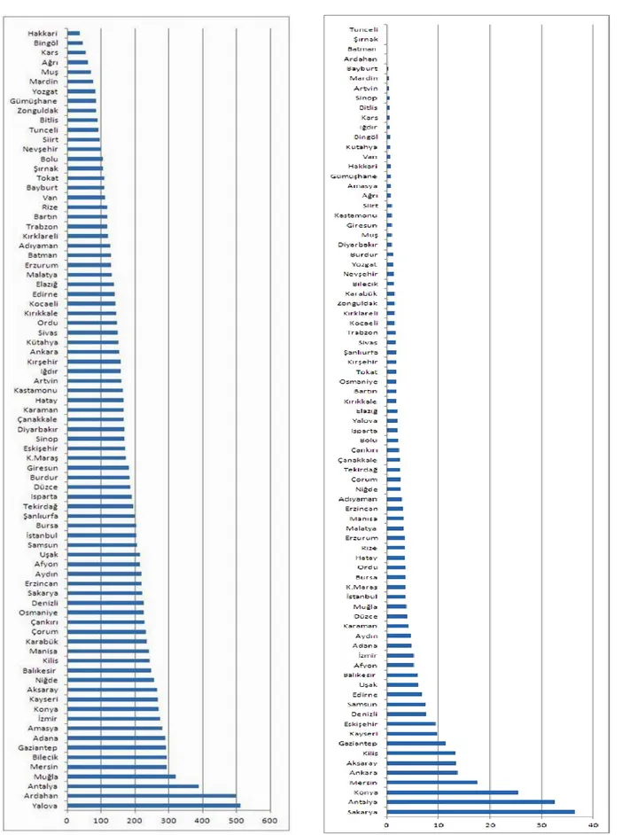
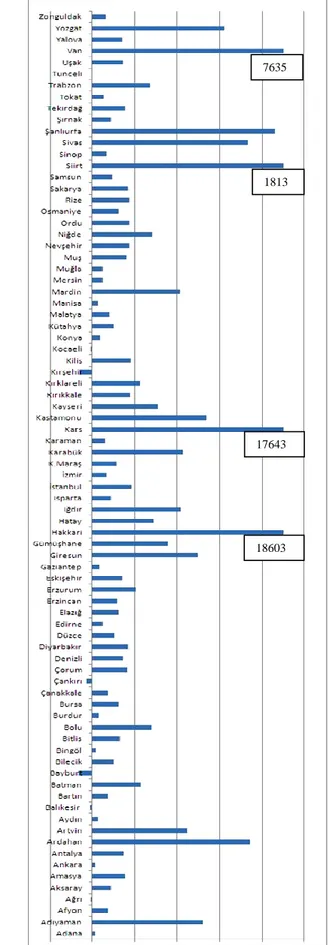
Türkiye'de mevcut mevzuata göre trafik denetimleri, İçişleri Bakanlığı Emniyet Genel Müdürlüğüne bağlı Trafik Denetleme Birimleri ile Jandarma Komutanlığına bağlı Jandarma Trafik Denetleme Birimlerinde görevli Trafik Zabıtasınca yapılmaktadır. Ayrıca, sürücülerin denetlenmesi faaliyetlerine yardımcı olmak üzere 1997 yılında hayata geçirilen ve gönüllülük esasına dayanan Fahri Trafik Müfettişliği sistemi mevcuttur. Türkiye’de trafik denetimlerinin ve cezaların ölüm, yaralanma ve kaza riskini azaltmadaki etkisini inceleyen az sayıda çalışma bulunmaktadır. Bu çalışmada, 2010-2013 yıllarını kapsayan 4 yıllık süreçte Polis ve FTM’ler tarafından sürücülere yazılan cezalar il düzeyinde karşılaştırmalı olarak incelenmiş, yazılan cezalar ile trafik kazalarındaki ölüm miktarı değişimleri bir arada değerlendirilerek trafik cezaları-trafik güvenliği ilişkisi ortaya konulmaya çalışılmıştır.
2. Yöntem
Çalışmada veriler 4 aşamada analiz edilmiştir. İlk aşamada, 2010, 2011, 2012 ve 2013 yıllarında 81 ilde meydana gelen kazalardaki ölü sayıları “Türkiye İstatistik Kurumu, İstatistik Yıllıkları”ndan, yine aynı yıllara ait, polis sorumluluk bölgesinde sürücülere yazılan cezalar ile FTM’ler tarafından sürücülere yazılan cezalar da “Emniyet Genel Müdürlüğü, Denetim Faaliyetleri Yıllıkları”ndan temin edilmiştir. İkinci aşamada temin edilen veriler Microsoft Excel programına aktarılarak bir veri tabanı oluşturulmuştur. Üçüncü aşamada verilerin birbirleri ile karşılaştırılabilmesi için 100.000 nüfus başına ölü [(ölü sayısı/nüfus)×100.000], 100.000 sürücü başına ölü [(ölü sayısı/sürücü sayısı)×100.000], 1000 sürücü başına ceza [(ceza sayısı/sürücü sayısı)×1000] değerleri dikkate alınarak değişkenler oluşturulmuştur. Son aşamada 100.000 sürücü başına ölü ve 1000 sürücü başına Polis ve FTM tarafından yazılan cezaların 2012-2013 yılları arasındaki değişimi hesaplanarak, 81 il için cezalar ve ölüm oranındaki artış ve azalış eğilimlerinin bir arada görülebileceği bir tablo hazırlanmıştır. Çalışmanın odağında Polis ve FTM’ler tarafından sürücülere yazılan trafik cezaları