THE IMPACTS OF THE KOSOVO WAR
ON NATO DEFENSE INDUSTRIES
A Master Thesis
By
EMİN ATEŞ
Department of Management
Bilkent University
Ankara
September 2002
THE IMPACTS OF THE KOSOVO WAR ON
NATO DEFENSE INDUSTRIES
The Institute of Economics and Social Sciences Of
Bilkent University
By
Emin ATES
In Partial Fulfillment of the Requirements for the Degree of
MASTER OF BUSINESS ADMINISTRATION in
THE DEPARTMENT OF MANAGEMENT BİLKENT UNIVERSITY
ANKARA September 2002
I certify that I have read this thesis and have found that it is fully adequate, in scope and in quality, as a thesis for the degree of Master of Business Administration.
--- Assist. Prof. Zeynep ÖNDER
I certify that I have read this thesis and have found that it is fully adequate, in scope and in quality, as a thesis for the degree of Master of Business Administration.
--- Assist. Prof. Aydın YÜKSEL
I certify that I have read this thesis and have found that it is fully adequate, in scope and in quality, as a thesis for the degree of Master of Business Administration.
--- Assist. Prof. Aslı BAYAR
Approval of the Institute of Economics and Social Sciences
--- Prof. Kürşat AYDOĞAN Director
ABSTRACT
THE IMPACTS OF THE KOSOVO WAR
ON NATO DEFENSE INDUSTRIES
Ateş, Emin
M.B.A., Department of Management Supervisor: Assist. Prof. Aydın Yüksel
September 2002
The purpose of this study is to examine the effects of the Kosovo War on the NATO countries defense industry stocks. The data set covers daily prices of stocks of 34 U.S., 12 U.K., 7 French and 3 Turkish companies, totaling 56 defense stocks. The analysis is conducted by using both standard event study methodology and multivariate regression model. The study provides evidence that the defense stocks reacted positively and significantly to the Kosovo War. The study shows that there is a significant difference between the abnormal returns of the U.S. defense stocks and European defense stocks. However, the analysis proves that there is no significant difference between the abnormal returns of aerospace stocks and non-aerospace defense stocks.
Keywords: The Kosovo War, event study, defense industry, multivariate
ÖZET
KOSOVA SAVAŞININ
NATO SAVUNMA SANAYİLERİNE ETKİSİ
Emin ATEŞ
YÜKSEK LİSANS TEZİ, İŞLETME FAKÜLTESİ Tez Danışmanı: Yrd.Doç. Dr. Aydın Yüksel
Eylül, 2002
Bu çalışmanın amacı Kosova Savaşının NATO ülkelerinin savunma sanayi hisselerine olan etkilerini araştırmaktır.Örneklem 34 Amerikan, 12 İngiliz, 7 Fransız ve 3 Türk olmak üzere 56 savunma sanayi şirketinden oluşmaktadır. Analizler olay etki çalışması ve çok değişkenli regresyon modeli ile yapılmıştır. Çalışma savunma sanayi hisselerinin Kosova Savaşı’na olumlu ve belirgin bir şekilde tepki gösterdiğini bulmuştur. Ayrıca çalışma, Amerikan ve Avrupalı şirketlerin anormal getirileri arasında belirgin bir fark olduğunu göstermiştir. Ancak, havacılık şirketleri ve diğer sektörlerdeki şirketlerin anormal getirileri arasında belirgin bir fark bulunamamıştır.
Anahtar Kelimeler: Kosova Savaşı,olay etki çalışması, savunma sanayi, çok
ACKNOWLEDGEMENTS
I am very grateful to Assist. Prof. Aydın Yüksel for his supervision, constructive comments, and patience throughout the study. I also wish to express my thanks to other committee members for their comments on the study. Finally, I am grateful to my wife and father, to whom this thesis is dedicated.
TABLE OF CONTENTS
Abstract ………. i
Özet ………. ii
Table of Contents ………. iv
List of Tables ………. vi
List of Figures ………. vii
CHAPTER 1: Introduction ………. 1
CHAPTER 2: The Kosovo War and NATO Defense Industries… 3
2.1 The Kosovo War: Review and Results ………. 3
2.2 U.S. and European Industries Comparison ……… 6
2.3 Aerospace Industry ……… 9
CHAPTER 3: Literature Review ………. 10
3.1 Market Efficiency ………. 10
3.2 Event Studies ……… 12
3.3 Studies Examining the Impacts of Wars ……….. 14
CHAPTER 4: Methodology and Data ……… 16
4.1 Hypotheses ……… 16
4.2 Methodology ………. 17
4.2.1 Standard Event Study Methodology …... 17
4.2.1.1 Defining Event Date …………. 18
4.2.1.2 Measuring Normal and Abnormal Returns 19 4.2.1.3 Statistically Testing the Abnormal Returns 22 4.2.2 Event Study Problems ……… 24 4.2.2.1 Standard Event Study Problems 25
4.2.2.2 Problems of Regulatory Event Studies 27
4.2.3 Jaffe Standardized Residual Test ………… 30
4.2.4 Multivariate Regression Model ………….. 31
4.1 Data ……… 36
CHAPTER 5: Results ……….. 40
5.1 Graphical Results ………..……… 40
5.2 Statistical Test Results ……….………… 43
5.2.1. Test of Hypothesis 1…….…..………… 43
5.2.2. Tests of Hypotheses 2 and 3……… 48
CHAPTER 6: Conclusion ……….. 54
LIST OF TABLES
Table 1 Final Cost of the Kosovo War………. 5 Table 2 Annual Defense Expenditures of NATO Members……… 6 Table 3 Major Arms Used in The Kosovo War……….. 8 Table 4 Summary of Hypotheses………. 17 Table 5 Chronology of Important Days for The Kosovo War……. 18 Table 6 Ratio of σX (Independence) / σX (Dependence) for Various
Levels of Cross-Correlation and Sample Sizes……… 29 Table 7 Distributions of Pairwise Correlations between ARs
Securities………. 29 Table 8 Hypotheses Testing in MVRM……….. 35 Table 9 Sample Companies List……… 38 Table 10 Chronology of Important Days for The Kosovo War… 42 Table 11 Test Of Hypothesis That The Event Had No Impact … 44 Table 12 Individual Parameter Estimates of MVRM…………. 46 Table 13 % Negative Reaction of Portfolios……….. 48 Table 14 Results of JSR Test and Average Effect Test of MVRM 49 Table 15 Results for the Comparison of U.S. and European Firms’
Reactions……….. 50 Table 16 Results for Market Value Comparison of U.S. and European
Firms Portfolios……… 50 Table 17 Results for the Comparison of Aerospace and Other Firms’
Reactions……….. 51 Table 18 Regression Results for the Comparisons …….……… 52
LIST OF FIGURES
CHAPTER 1
INTRODUCTION
In 1989, the first sparks of the Kosovo conflict are seen when the autonomy of the region is removed. After nine years, the conflict turned into an ethnic cleansing. NATO had to intervene the conflict for the stability of the region.
Although the cost of the war was high, it created new opportunities for marketing and selling defense products. Therefore, it is expected that the war affected defense industry firms positively. During the war, the superiority of U.S. products was observed. The feature of the Kosovo War is that it was mainly an air campaign. So it is expected that U.S. firms and aerospace firms benefited more than European firms and the firms that are not in the aerospace industry.
In this study, the impacts of the Kosovo War on NATO member countries’ defense stocks are investigated by using event study methodology. This is the first study that investigates the financial impacts of Kosovo War.
Event studies measure the impact of a specific event on the value of a firm by using financial market data (MacKinlay 1997). They are concerned with measuring abnormal returns around the date of the specific event. The role of news as determinant of stock returns has been the subject of interest, because efficient market hypothesis assumes that stock returns fully reflect all available information and adjust immediately to the arrival of new information. (Shapiro 1999) Thus, a measure of the event’s economic event impact can be constructed using security prices observed over a relatively short time period.
In order to measure the effects of this war on the defense firms of NATO countries, first the standard event study methodology is employed. The cumulative abnormal returns obtained are used to interpret the general effects of the Kosovo War.
As events, wars are similar to regulatory changes. The first similarity is that there is no single event date like those in merger announcements or stock splits. There are many days until the beginning of the war that increase the expectations of a war. The second similarity is that the event date is same for all firms and all of the firms are in the same industry. Same event date and the same industry issues create statistical problems that challenge the adequacy of using standard event study methodology to examine these types of events. Therefore, ten important dates were chosen and then Jaffe Standardized Residual Test (JSR) and Multivariate Regression Model (MVRM) are employed to deal with these problems.
The results of the analysis show that, defense companies reacted to the Kosovo War. The evidence indicates that the stocks of defense companies reacted positively and significantly to the attack of the Serbian Army to Albania. There is a significant difference in the reactions of U.S. and European firms portfolios to this event. However, the difference in the reactions of aerospace firms and the firms in other sectors is not significant.
CHAPTER 2
THE KOSOVO WAR & NATO DEFENSE INDUSTRIES
This chapter starts with a brief review of the Kosovo War. The rest of the discussion focuses on two major observations regarding the military capabilities of NATO member countries and the importance of the aerospace division within the defense industry.
2.1 The Kosovo War: Review and results
Kosovo lies in southern Serbia and has a mixed population of which the majority is ethnic Albanians. Until 1989, the region had a high degree of autonomy within the former Yugoslavia. In 1989, Serbian leader Milosevic altered the status of the region by removing its autonomy. Then, Kosovar Albanians were exposed to discrimination, since they opposed to the removal of autonomy. After nine years, discrimination turned into a systematic violent ethnic cleansing, and 1,500 Kosovar Albanians were killed and 400,000 people were forced to leave their homes in 19981.
These incidents led to the first international meeting for the Kosovo conflict, which was held on 28 May 1998 by foreign ministers of NATO countries. The next meeting was held on 12 June 1998 by the NATO Council. The alternative of solving the problem by a military operation was first consulted in this meeting. Following the deterioration of situation, on 13 October 1998, the NATO council authorized
Activation Orders2 for air strikes. At the last moment, the Serbian government agreed to comply and air strikes were called off.
Despite all past efforts, the situation in Kosovo flared up again at the beginning of 1999. Renewed international efforts were made to give new political impetus to the solution of the conflict. For this reason, the six-nation Contact Group3 and NATO declared the agreement on air strikes. Subsequently, the six-nation Contact Group established meetings in Paris, in February and March 1999. At the end of these meetings, the Kosovar Albanian delegation signed the proposed peace agreement, but the talks broke up without the signature of the Serbian delegation. Immediately afterwards, Serbian military and police forces stepped up the intensity of their operations against ethnic Albanians in Kosovo.
After a final ultimatum to Serbia, either to stop attacks or to face imminent NATO air strikes, which the Serbian government refused to comply with, the final order was given to start the air strikes on 23 March.
After an air campaign lasting seventy-eight days, the full withdrawal of Serbian forces from Kosovo began in June 1999. On the same day, the United Nations Security Council passed a resolution welcoming the acceptance by the Federal Republic of Yugoslavia of the principles on a political solution to the Kosovo crisis.
The Kosovo War was the largest combat operation in the history of NATO. Its cost was $ 49.27 billion. Only military costs reached to $ 4 billion.
During the conflict, NATO:
2 It is an order to be ready to attack when the final order is given.
3 The sixnation Contact Group consists of France, Italy, Germany, Russia, United Kingdom and United States
• Dropped more than 23,000 bombs and missiles
• Spent more than $ 225 million on fuel in the first week
• Destroyed almost half of the Yugoslavia’s industrial production
• Caused $ 2.61 billion damage to the Yugoslavian economy, according to Serbian experts.4
Table 14
Final Cost of Kosovo War
THE WAR $ 4.09 bn. AID $ 3.95 bn. PEACEKEEPING $ 9.33 bn. RECONSTRUCTION $ 31.89 bn. TOTAL $ 49.27 bn.
Table 1 decomposes the components of the total cost of the Kosovo War. It shows that the most important cost is reconstruction cost for the Federal Republic of Yugoslavia, and it is approximately 32 billion dollars. The costs for United Nations and other countries are about 13 billion dollars as the sum of aid and peace keeping costs. The cost of the war is approximately 4 billion dollars for NATO.
When the war is reviewed, two important observations can be made. Firstly, the gap between the military capabilities of the U.S. and its allies became clear. Secondly, it was the first instance, in which victory was won only by air forces. These issues will be covered in the next two sections in more detail.
2.2 U.S. and European Defense Industries Comparison
The Kosovo conflict made U.S. material and technological dominance within the NATO Alliance significantly apparent. In fact, the main reason is not that Europe lacks the military technological talents of the United States. The real causes of the gap are the disparity in their military spendings, and the differential treatment of the defense industry by the U.S. administration.
When the first reason is examined, it will be seen that there is a huge difference between the defense expenditures of the U.S. and European countries. Table 2 displays the annual defense expenditures of the U.S. and Europe as a whole.
Table 2
Annual Defense Expenditures of NATO Members
1996 1997 1998 1999 2000 Total NATO Europe (US $) 186.821 172.732 175.306 179.671 164.559
United States (US $) 271.417 276.324 274.278 280.969 296.373
Total NATO (US $) 466.681 456.879 457.112 468.960 468.999
Note: Numbers are X 100.000
Total NATO Europe is the sum of 16 European Countries’ Expenditures Total NATO is the sum of Total NATO Europe, United States and Canada
Expenditures
According to Table 2, the U.S.’s expenditures are almost twice the sum of 16 European countries’ expenditures. It should be taken into consideration that the U.S. spends 60% of this money on research and development (R&D) activities5. The money spent by the U.S. on R&D is equal to total military expenditures of all
Europe. Therefore, U.S. material and technology is more advanced than those of Europeans. This gives U.S. defense companies an advantage over European defense companies in the international arms market.
The second reason of the gap is the governmental support to the defense industry companies in the U.S. If it is investigated, it can be noticed that unlike its intension to limit mergers in other industries through the use of the antitrust law, U.S. government encourages mergers in the defense industry. Because U.S. Department of Defense is both the principal buyer and the main regulator of the defense industry, mergers in the defense industry raise complex competition policy issues that are not easily resolved by applying conventional antitrust merger analysis techniques. (Kovacic and Smallwood 1994). Therefore, the issue that the U.S. pays attention to is not the cost, but the competence and technological superiority of the materials. This stimulates the companies to manufacture innovative products.
Table 3 shows the major arms used in the Kosovo War. Although we do not have data on how $ 4.1 billions spent on weapons is allocated among the defense companies of different countries, we can predict that the U.S. encouraged the use of weapons produced by its own companies.
Depending on the disparities mentioned above, it is likely that there is a difference between U.S. and European defense industry companies regarding the impact of the Kosovo War on them.
Table 3
Major Arms Used In The Kosovo War
Name Type Producer
E-3 Sentry C3a Aircraft U.S. F-117 A Stealth Fighter Aircraft U.S.
F-16 Fighter Aircraft U.S. F-15 Fighter Aircraft U.S. B-52 Bombardment Aircraft U.S. B-1 BOMBER Bombardment Aircraft U.S.
B-2 Bombardment Aircraft U.S. Tomahawk Cruise Missile U.S.
AGM-65 Maverick Guided Missile (ATS)b U.S. AGM-86 C Guided Missile U.S. AGM-88 Guided Missile (ATS) U.S.
GBU-15 Glide Weapon U.S. AGM-130 A Guided Missile (ATS) U.S.
GR-7 Harrier Fighter Aircraft U.K.
Sidewinder Guided Missile U.K. L-1011 TriStar Cargo Aircraft U.K.
Jaguar Fighter Aircraft U.K. & France Tornado Fighter Aircraft U.K. KC-130 Tanker Aircraft Spain KC-10 Cargo Aircraft Spain Source: http://abcnews.go.com/sections/world/DailyNews/kosovo_costs990326.html a. Command, control and communication
2.3 Aerospace Industry
The Kosovo War became exclusively an air campaign6. Unlike a traditional military conflict, there was no direct clash of massed military forces. Air attacks lasted 78 days on selected strategic targets to degrade the ability of the Federal Republic of Yugoslavia (FRY) military to perform its functions. The Kosovo War, therefore, became the first instance in which victory had been realized through the exclusive application of air power.
The developments and changes in technology affected warfare strategies and tactics. The most important component of military power is the air forces in our age. Therefore, it can be observed that the aircraft development absorbs much of the defense spending of countries7. This directly influences aerospace industry financial figures.
Depending on the structure of the Kosovo War, it is likely that there is a difference between the aerospace industry companies and the companies in non-aerospace industries regarding the impact of the Kosovo War on them.
6 Table 3 demonstrates the arms used in the Kosovo War and it can be easily seen that it consists of aircrafts and missiles.
CHAPTER 3
LITERATURE REVIEW
In this chapter, the market efficiency concept is covered first as a background for event studies. Next, a brief discussion of event study literature is presented. A review of the event studies examining the impacts of wars and military actions concludes the chapter.
3.1 Market Efficiency
Market efficiency implies that stock prices reflect all available relevant information in the market. A capital market is said to be efficient, if it fully and correctly reflects all relevant information in determining security prices.
Fama (1970) presented three strictly increasing degrees of information processing efficiency, based on how much of the available public and private information market prices are expected to reflect.
In the weak-form efficiency, asset prices incorporate all historical information. This form of efficiency implies that trading strategies based on analyses of historical pricing trends or relationships cannot consistently yield excess returns to investors. Since prices are “memoryless”, they are unforecastable, and will only change in response to the arrival of new information. This implies that asset prices follow a random walk, meaning that there is no correlation between subsequent price changes, and the asset prices fluctuate randomly and unpredictably.
In semi-strong form efficiency, asset prices incorporate all publicly available information. The level of asset prices should reflect all relevant historical, current and forecastable future information that can be obtained from public sources. Also in this form of efficiency, asset prices should change fully and instantaneously in response to the arrival of relevant new information. The key point about this form of efficiency is that it only requires information that can be collected from public sources to be reflected in asset prices.
In strong-form efficiency, asset prices reflect all information – public and private. This is an extreme form of market efficiency, because it implies that important company-specific information will be fully incorporated in asset prices with the very first trade after the information is generated and before it is publicly announced. In strong-form efficient markets, most insider trading would be unprofitable.
Fama (1991) renamed the market efficiency categories: tests for return predictability, event studies, and tests for private information instead of weak form, semi-strong form and strong form, respectively. While the coverage of semi-strong and strong form efficiencies are the same as before, Fama added dividend yields and interest rates to the coverage of weak form efficiency.
In this study, markets are accepted as semi-strong form efficient, and price adjustments to public information (the Kosovo Conflict) are investigated in an event study framework.
3.2 Event Studies
Event studies measure the impact of a specific event on the value of a firm by using financial market data (MacKinlay 1997). They are concerned with measuring abnormal returns around the date of an event that is specified. The role of news as determinant of stock returns has been the subject of interest, because efficient market hypothesis assumes that stock returns fully reflect all available information and adjust immediately to the arrival of new information. (Shapiro 1999) Thus a measure of the event’s economic impact can be constructed using security prices observed over a relatively short time period.
Event studies have emerged as the single most important tool of empirical finance research due to their ease of use, clarity of purpose, flexibility, and absence of confusing influences (Megginson 1997). Event studies have a long history. According to MacKinlay, perhaps the first published study belongs to James Dolly (1933). Over the decades from the early 1930s until the late of 1960s, the level of sophistication of event studies increased. The improvements included removing general stock market price movements and separating out confounding events. The methodology that is essentially the same as that which is in use today was introduced in late 1960s.
Event studies have several major strengths. First, a researcher is able to gain an unbiased assessment of stock prices reaction to a given event by averaging out random noise over many different observations. Second, event studies are very clean tests that yield unambiguous results. Third, event studies provide a direct test of semi-strong form market efficiency, since they allow one to determine if information is incorporated fully and instantaneously into stock prices. (Megginson 1997)
The event study has many applications. In accounting and finance research, event studies have been applied to a variety of firm specific and economy wide events. Some examples include mergers and acquisitions, earning announcements, issues of debt or equity, regulatory changes and announcements of macroeconomic variables such as the trade deficit, and political events such as wars. In majority of applications, the focus is the effect of an event on the price of a particular class of securities of the firm, most often common equity. (MacKinlay 1997)
Event studies can be used for different purposes: Market efficiency studies assess how quickly and correctly the market reacts to a particular type of information. Information usefulness studies assess the degree to which company returns react to the release of a particular bit of news. In a metric explanation study, the metrics are explained by splitting the sample into different subsamples and examining whether the unusual element of returns differed among the subsamples. The types of event studies can be classified as market efficiency, information value and metric explanation studies.
Besides those three types, methodology studies of event study design can be accepted as a fourth type. (Henderson 1990) The methodology studies consider how best to run event studies. MacKinlay (1997) describes and discusses the procedures of standard event study methodology. He defines models and brings up some problems shortly. Henderson (1990) differs from MacKinlay in that he focuses in a detailed way on the problems and the approaches to deal with those problems in event studies. Binder (1998) discusses the statistical power of the standard methodology in different applications and explicates the multivariate regression framework. Collins and Dent (1984) make a comparison of alternative testing methodologies in event studies by means of simulation.
3.3 Studies Examining The Impacts Wars And Military Actions
Previous studies examine a wide variety of news events and their effects on aggregate stock prices. The discussion in this section is limited to studies dealing with the impacts of wars.
McDonalds and Kendall (1994) examined the effects of political events in the stock market. The stock price behavior of 16 U.S. defense industry firms was examined before and after 17 unforeseeable political events involving military forces. Their findings reveal that stock prices for defense firms tend to rise as a result of military actions. The events, as expected on the whole, appear not to have been anticipated. The most important effect on the U.S. defense industry stocks was observed for those events involving the former Soviet Union. Actions undertaken by the USSR were accompanied by dramatic increases in the U.S. defense industry stock prices.
Attia (1998) investigated the impact of the Iraqi invasion of Kuwait, and the Persian Gulf War on the stock prices of petroleum companies operating in the Gulf countries. His results provide evidence that the OPEC production had statistically significant influence on the average monthly index of multinational petroleum companies. In addition, average stock prices of multinational petroleum companies are significantly higher during August 1990 (the month of Iraqi invasion of Kuwait) than those during months before and after August. However, he could not find a significant difference between the average stock prices during the overall war period and the average stock prices before and after the war period.
Shapiro (1999) used a portfolio approach to examine the response of defense shares to war –and peace – related news. Consistent with other studies, the majority of the evidence confirms that the outbreaks of war, or announcements that increase the probability of a war commencing, are accompanied by positive abnormal returns. His study included a larger number of firms than those in previous studies. He built defense portfolios according to companies’ R&D levels and found that the companies with high levels of R&D realized higher positive abnormal returns. Although he did not justify his results about R&D, it is supposed to be because R&D-oriented companies have more chance to introduce and promote new products when the market for defense products grows.
Cantenar (2000), like Attia (1998), chose the intervention of the U.S. to the Gulf Crisis as the major event and investigated the impact of this event on U.S. defense stocks by using event study methodology. His sample included thirty-nine defense firms selected from the U.S. Department of Defense top contractors list. His analysis of the abnormal returns on defense stocks showed that the U.S. military intervention to the Gulf crisis affected those stocks significantly and positively in both short and long terms. He extended his study to find if there was a difference in the reactions of firms according to companies’ defense dependency ratio (the ratio of military sales to total sales) and market value. He found a positive relationship between defense dependency ratio and abnormal returns of defense firms, controlling for the size of the firm.
CHAPTER 4
METHODOLOGY AND DATA
4.1 Hypotheses
The role of news (events) as a determinant of stock returns is our subject of interest because the efficient market hypothesis assumes that stock returns reflect all available information and adjust immediately to the arrival of new information. The first hypothesis checks whether the returns of NATO member countries defense stocks react to the Kosovo War.
The Kosovo War proved that there is a considerable difference between U.S. and European military capabilities due to supremacy of U.S. technology and application. During the Kosovo War, superior U.S. products must have been used. Therefore, U.S. companies must have gotten the lion’s share from new orders. It is expected that there would be a difference between the abnormal returns of U.S. and European companies. Thus, it is hypothesized that there is no difference between abnormal returns of U.S. and European defense industry companies as the second hypothesis of the study.
The Kosovo War took its place in history as the first battle executed and accomplished only by air forces. Therefore, the air forces captured the biggest slice from the defense spendings during this war. It is expected that the aerospace companies react to this event differently than the non-aerospace companies. So the last hypothesis is that there is no difference between the abnormal returns of aerospace companies and other defense companies.
Table 4 depicts the summary of hypotheses that will be tested in this study.
Table 4
Summary of the Hypotheses
• H10 : NATO countries defense industry stocks do not react to the Kosovo War
H1A : NATO countries defense industry stocks react to the Kosovo War • H20 : Average reactions (abnormal returns) of U.S. defense companies are
equal to the average reactions (abnormal returns) of European defense companies during the Kosovo War.
H2A : Average reactions of U.S. defense companies are not equal to the average reactions of European defense companies during the Kosovo War. • H30 : Average reactions of aerospace companies are equal to the average
reactions of non-aerospace companies during the Kosovo War.
H3A : Average reactions of aerospace companies are not equal to the average reactions of non-aerospace companies during the Kosovo War.
4.2 Methodology
In this section, standard event study methodology and its problems are reviewed first. Then, due to the similarity of the Kosovo War to regulatory changes, the problems encountered in conducting event studies to examine regulatory changes are covered. Finally, two methods proposed to deal with these problems, namely Jaffe Standardized Residual Test and Multivariate Regression Model are discussed.
4.2.1 Standard Event Study Methodology
While there is no unique structure for conducting event studies, there is a general flow of analysis. Henderson (1990) and MacKinlay (1997) define the event study steps similarly. These steps are as follows:
2. Measuring normal and abnormal returns. 3. Statistically testing the abnormal returns.
4.2.1.1 Defining the Event Date
After defining the event, it must be determined when it took place. This may seem simpler than it is. The issue is not when an event occurred, but when the market, that is, its most interested and well informed segment, could have reasonably anticipated the news.
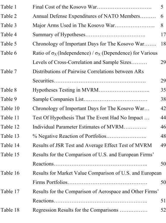
The same holds for the Kosovo War. There are eight incidents including meetings and negotiations until the last day of the Kosovo War. Table 5 provides a list of events included in the analysis. Selection of these dates is based on the belief that occurrences on these dates provided information concerning the probability that war would begin. In addition, the last day of the war is included to the analysis to see the effects of the end of the war.
Table 5
Chronology of Important Days for The Kosovo War
Date Event
12 June 1998
NATO Meeting At Defense Ministry Level First Time For Consideration Of Military Options To Kosovo 13 October 1998 Authorization Of "Activation Orders" For Air Strikes
30 January 1999 NATO And Contact Group Decision For Air strikes
06-23 February 1999 1rst Round Of Paris Negotiations Between Albanians And Serbians 15-18 March 1999 2nd Round Of Paris Negotiations Between Albanians And Serbians
20 March 1999 US Ambassador Flew Belgrade To Warn For Air Strikes 23 March 1999 Air Strikes Began
On 12 June 1998, the NATO Council, meeting at Defense Minister level, asked for an assessment of possible further measures that NATO might take for the Kosovo crisis. This led to the consideration of a large number of possible military options. On 13 October 1998, following a deterioration of the situation, NATO Council, authorized Activation Orders for air strikes. This move was made to support diplomatic efforts, and it worked out. The Serbian government agreed to comply and the air strikes were called off. On 29 January 1999, Six Nation Contact Group agreed to convene urgent negotiations between parties to the conflict, under international mediation. NATO supported Contact Group efforts by agreeing on January 30 to the use of air strikes if required, and by issuing a warning to both sides in the conflict. As a result of NATO’s warnings, on dates 6-23 February and 15-18 March 1999, Paris negotiations were organized. As the final attempt, on 20 March 1999, the U.S. Ambassador flew to Belgrade to warn for air strikes. Serbia refused to comply and on 23 March 1999 air strikes began. On 10 June 1999, air strikes were terminated.
4.2.1.2 Measuring Normal and Abnormal Returns
In order to calculate normal and abnormal returns, event window and estimation window must be determined. The estimation window is the period chosen to generate expected returns during the event window. The event window is the period over which security prices of firms involved in this event will be examined. The event window is the event day plus and minus some number of days, weeks or months observed to see if anything unusual happened.
The event windows and estimation windows in previous studies differ from each other. Cantenar (2000) defined his event window as 253 days, which included the event day and 252 days (one year) after the event. He used an estimation window of 250 days, which ends 20 days before the event date. Shapiro (1999) focused on a fairly short window: event day and next five trading days. Shapiro used 180 trading days until 40 days before the headline date as his estimation window. MacKinlay (1997) employed a 41-day event window, comprised of 20 pre-event days, the event day and 20 post-event days. He used 250 trading days period prior to the event window as the estimation window. Megginson (1997) proposed a very narrow event window to determine what the immediate reaction to the event is. He suggested the period from 150 days to 20 days before the event day as the estimation window. McDonalds and Kendall (1994) defined their event window as 181 days around (90 days before the event date, event day and 90 days after the event day) the event day. They used 200 days period before the event window as their estimation period. It can be easily seen that there is not a precise consensus on the periods.
In this study, there is not a single event and single event window. There are multiple events and the event windows are three days – one day before the event, event day and one day after the event – for each event. In order to examine the short-term effects of events, event windows are taken as three days.
It is typical for the estimation window and the event window not to overlap. Estimation window must be before, after or both before and after some times the event window. Including the event window in the estimation of the normal return parameters could lead to the event returns’ having a large influence on the normal return measure. In this situation, both normal returns and abnormal returns would capture the event impact. This would be problematic, since the methodology is built
on the assumption that the event impact is captured by the abnormal returns (MacKinlay 1997).
Therefore, estimation window which is taken as 180 days, ends three days before, 12 June 1998, the first important event date for The Kosovo War, in order to prevent event and estimation windows to overlap.
For the discussion of the methodology, some terms need to be defined. Normal return is defined as the return that would be expected if the event did not take place. Abnormal return is the mathematical difference between observed return and normal (expected) return for that day, week or month.
There are several approaches for describing a firm’s normal returns. Some common ones are: mean returns, market adjusted returns and market returns. In the mean returns approach, a company’s returns in the estimation period are averaged. In the event window, the company is expected to generate the average return as the normal return. In the market adjusted returns model, a company, in the absence of news, is expected to generate the same returns as the market during event window. The method is used especially to examine the effects of initial public offerings since this it does not require an estimation window. The abnormal return for market adjusted model is calculated as follows:
AR
it= R
it– R
mt(1)
where Rit and Rmt are the period-t returns on security i and the market portfolio,
respectively.
The market model that is used in this study is a statistical model, which relates the return of any given security to the return of the market portfolio. This
method considers the risk of the security and the movement of the market during the event period. For any security i the market model is:
R
it= α
i+ β
iR
mt+ ε
i(2)
where Rit and Rmt are the period-t returns on security i and the market portfolio,
respectively. αi and βi are the parameters of the market model and εi is the
prediction error. αi and βi parameter estimates are obtained from the regression
model in equation (2) using estimation period data. Given the market model estimates, the abnormal returns are found for the event period. Using the market model to measure the normal return, the sample abnormal return is:
AR
it= R
it– α
i– β
iR
mt(3)
4.2.1.3 Statistical Tests of the Abnormal Returns
Before testing, abnormal returns must be aggregated both across firms and across time. Aggregation over time is a simple accumulation over the event window. In event studies, all time is kept relative to the event date. The cumulative abnormal return (CAR) is the sum of all the abnormal returns between the event date and day T. CAR is computed for each firm as of time T as follows:
∑
= = T t it iTAR
CAR
1(4)
Aggregation across firms involves the averaging of CARs for all firms in the sample on a given day in the event window. The average cumulative abnormal return ( CAR ) on a day T for N securities is defined as:
∑
=
= N i iT TCAR
N
CAR
1 1(5)
where CARiT is the cumulative abnormal return for the ith security until day T
starting from the event day.
The last step in the event study is statistical testing of aggregated returns. Early event studies often used graphics as the primary method of interpretation. CAR plots were presented to show the reader how the firms reacted to an event. Such pictures are still routine in event studies. But now, the results should be supported by statistical tests.
To test the null hypothesis that the mean cumulative abnormal return is equal to zero for a sample of N firms, t statistic is employed as described in Barber and Lyon (1997):
(
CAR N)
TCAR
t
T CARσ
=(6)
where CART is the average cumulative abnormal return and σCAR is the
cross-sectional sample standard deviation of cumulative abnormal returns for the sample of N firms. When the sample is drawn randomly from a normal distribution, this test statistic follows a Student’s t-distribution under the null hypothesis. The Central Limit Theorem guarantees that if the measures of abnormal returns in the cross-section of firms are independent and identically distributed drawings from finite variance distributions, the distribution of the mean abnormal return measure converges to normal as the number of firms in the sample increases. (Barber and Lyon 1997)
The method discussed to this point is parametric, in that specific assumptions have been made about the distribution of abnormal returns. However, non-parametric approaches, which are free of specific assumptions concerning the distribution of returns, are also available.
Typically, non-parametric tests are not used in isolation but in conjunction with their parametric counterparts. The inclusion of the non-parametric tests provides a check of the robustness of conclusions based on parametric tests.
In this study, Wilcoxon Signed Rank test is used to examine the significance of cumulative abnormal returns. This test is based on ranks. The hypothesized median (zero in our case) is subtracted from each observation. After subtraction, any result of zero is discarded. And then the absolute values of remaining non-zero differences are ranked. If two or more absolute differences are tied, the average rank is assigned to each. The ranks corresponding to positive differences are summed to find the Wilcoxon statistic Rt. Expected value and standard deviation for sum of
ranks are defined as:
( )
(
)
4 1 + =N
N
R
t E(7)
( )
(
)(
)
24 1 2 1 + + =N
N
N
R
t σ(8)
For N>12 the distribution of the following statistic can be adequately approximated by the standard normal:
( )
( )
R
R
R
Z
t t t t E σ − =(9)
4.2.2 Event Study Problems
In this section, event study problems will be discussed in two parts. In the first part, standard event study methodology problems will be covered. In the second part, the problems of regulatory event studies will be discussed due to the Kosovo War’s similarity to regulatory events.
4.2.2.1 Standard Event Study Problems
After defining the event, a researcher must determine when it took place. Misidentification of an event date can obscure an issue. Early merger studies used the date of a merger and found no significant evidence of shareholder return effects. Later studies, on the other hand, used the date on which the intent to merge was announced, and, they found significant abnormal and cumulative abnormal returns.
Having decided on the event date, the estimation period must be determined. There are three choices for the estimation period: before, after and around the event window. The majority of studies used an estimation period before the event. The problem with the estimation window is that it should not overlap event window to eradicate event’s effects on the normal return calculation.
In addition to these procedural issues, there are some econometric problems. Regression models are based on a number of statistical assumptions. Specifically, the models assume that the residuals: are normally distributed with a mean of zero, are not serially correlated, have a constant variance, and are not correlated with the explanatory variables. Further, when regression system is used, it is also assumed
that there is no correlation between residuals for the different firms. However, there is reason to be concerned about each of these assumptions.
Non-normality: the non-normality problem is potentially more troublesome for studies using daily data, because daily returns are non-normal. Fortunately, the same is not true for residuals, since the distribution of residuals should be close enough to normal.
Autocorrelation and Non-synchronous trading: there may be statistically significant autocorrelation in the residuals.8 Non-synchronous trading – the mismatching of the values for Rmt and Rit owing to trading frequencies – creates bias
in betas of individual securities. The result is that the betas of infrequently traded securities are downward biased, while shares trading with more than average frequency have upward biased betas. (Henderson 1990) Unfortunately, the extra work for autocorrelation and non-synchronous trading does not seem to strengthen event study results.
Variance shifts: when the method of cumulating abnormal returns across firms and then aggregating in time is used, it is assumed that the variance does not change during the event window. When there are variance shifts, this assumption does not hold. In order to solve problems about variance shifts, the use cross-sectional variance is suggested, but there are costs to using such cross-cross-sectional measures. Such a calculation implicitly assumes that the variance for every firm is the same on day t and the estimates ignore estimation period data.
Event (calendar) clustering and correlation between residuals: calendar clustering refers to events occurring at or near the same time. Industry clustering refers to events concentrated in the same industry. Both event and industry
clusterings cause to reject the hypotheses more often in standard event study methodology by leading to correlation between residuals.
This problem will be discussed in a more detailed way in the next section.
4.2.2.2 Problems of Regulatory Event Studies
Three features of regulatory events make them more difficult to analyze than other types of events. (Binder 1985b) First, for many important regulations it is not accurately known when expectations change. Unlike stock splits or similar simple events, regulatory events usually involve no single well-defined announcement; rather there are multiple announcements, such as committee or senate approval during the legislative or administrative process. Regulatory announcements are also more likely to be anticipated than are corporate announcements. Because of the size of potential wealth transfers, there are extensive negotiations between interest groups and politicians of regulation before the actual voting; therefore the outcome is likely to be known ahead of time.
Second, it is not clear a priori that the effects of regulation are consistently positive or negative: in the same industry some firms may gain while others lose. Protective regulation can take a variety of forms and choice of form may affect differently the welfare of industry members. When there is this asymmetry, the usual tests of the significance of average or cumulative average returns will often falsely reject the hypothesis that regulation has an effect.
Finally, unlike other events that are most often studied, regulation often affects firms in the same industry during the same calendar time periods. Therefore,
when significant excess returns are found, it is not certain that whether these are due to regulation or to some other industry-specific shock.
These characteristics are valid for the Kosovo War as well. There are many negotiations and meetings that possibly changed the expectations and anticipations before the beginning of the war9. It is expected that firms react differently to the war. All firms are in the defense industry and the event date is same for all firms.
The event clustering and industry clustering lead to cross-sectional correlations of the dependent variable of interest (Collins and Dent 1984). Testing procedures, which fail to take cross-sectional correlations into account, can lead to unwarranted inferences. In order to provide some insights into the potential severity of the cross-sectional correlation problem, Collins and Dent (1984) computed the degree of bias for different sample sizes and levels of correlations. Table 6, taken from this study, illustrates that both sample size and the level of cross-correlation affect the degree of bias in the standard deviations of the sampling distribution of average portfolio abnormal returns.
Table 7 shows the distribution of correlations between abnormal returns of securities in this study. This information can be used for estimating the degree of bias. The mean level of cross-correlations is 0.057 and the sample size is 56 securities, estimation procedures yield estimates of σx (average standard deviation of
abnormal returns of sample securities), which are approximately 60% of the true or correct value10. The statistical tests of standard event study methodology based on σx
can lead to biased test results due to understating the standard deviation. Therefore, Jaffe Standardized Residual Test (JSR) and Multivariate Regression Model (MVRM) will be employed to deal with the cross-correlation problem.
9 Table 5 shows the important dates for the Kosovo War. 10 60% is calculated via interpolation by using Table 7.
Table 6
Ratio of σX (Independence) / σX (Dependence) for Various Levels of
Cross-Correlation and Sample Sizes
Sample Size Level of Correlation 5 10 20 40 60 80 100 0.00 1.0000 1.0000 1.0000 1.0000 1.0000 1.0000 1.0000 0.10 0.8452 0.7255 0.5872 0.4518 0.3807 0.3352 0.3029 0.20 0.7454 0.5976 0.4564 0.3371 0.2795 0.2440 0.2193 0.30 0.6742 0.5199 0.3863 0.2806 0.2312 0.2012 0.1805 0.40 0.6202 0.4663 0.3410 0.2454 0.2016 0.1751 0.1569 0.50 0.5774 0.4264 0.3086 0.2209 0.1811 0.1571 0.1407 0.60 0.5423 0.3953 0.2840 0.2024 0.1657 0.1437 0.1287 0.70 0.5130 0.3701 0.2644 0.1880 0.1538 0.1333 0.1193 0.80 0.4879 0.3492 0.2485 0.1762 0.1440 0.1248 0.1117 0.90 0.4663 0.3315 0.2351 0.1664 0.1360 0.1178 0.1054 σX (Independence)= (1/ N) σ2 σX (Dependence)= (1/ N) σ2 + ((N-1) / N) σi j where:
N = number of securities in sample
σ 2 = average variance of abnormal returns of sample securities
σi j = average covariance of abnormal returns of sample securities equal to ρ σi σj σX (Independence) / σX (Dependence) = 1/ √1+(N-1) ρ
Table 7
Distribution of Pairwise Correlations Between Abnormal Returns of Sample Securities
Mean Median StDev
t-statistic 0.0566 0.045 0.1026 4.12 Deciles Min. 0.1 0.2 0.3 0.4 0.5 0.6 0.7 0.8 0.9 Max. -0.211 -0.058 -0.025 0.001 0.023 0.045 0.065 0.092 0.132 0.190 0.969
4.2.3 Jaffe Standardized Residual (JSR) Test
This testing methodology uses a portfolio approach in the estimation of abnormal returns. In order not to be influenced by the correlations between abnormal returns of securities, the residual variance of an equally weighted portfolio of securities is measured. The residual variance of this portfolio is measured over an estimation period and it is used in testing the significance of the abnormal returns in the event window as follows: for each point, t, in the estimation period the abnormal returns from equation (3) are aggregated across the N securities to form average abnormal return (AAR) of portfolio in period t:
∑
= = N i it tAR
AAR
N 1 1for t = 1,…, T
(10)
The variance of the average abnormal returns is then computed as:
∑
−
= − = T tAAR
tAAR
T AAR 1 2)
(
1 1 ) var((11)
where∑
= = T tAAR
t T AAR 1 1(12)
and (1,T) is 180-day estimation period.
For the case where all securities in the sample experience the critical event at the same point in calendar time, the JSR test is:
S
AAR
AAR
t
~ t
N-1
(13)
4.2.4 Multivariate Regression Model
Rather than modeling abnormal returns as prediction errors from the market model equation, the sample period can be extended to contain the event period and (when there is only one event) a zero-one variable Dt can be included in the return
equation:
R
it= α
i+ β
iR
mt+ γ
iD
t+ u
it(14)
The coefficient γi is the abnormal return for security i during period t and is directly
estimated in the regression. That is, this approach parameterizes the abnormal return in the market model regression equation. This model can be adapted to equally weighted portfolio of firms, all of which experienced the events during the same calendar periods:
R
pt= α
p+ β
pR
mt+ γ
pD
t+ u
pt(15)
When an equally weighted portfolio is used as the dependent variable, γp gives the
estimate of the average abnormal return across the stocks in the portfolio. Alternatively, when there are multiple events, different dummy variables can be used for each event.
Tests of the hypothesis that the event affected security prices, based on the estimated gammas in equation (15), will not be very powerful when abnormal returns differ in sign across the sample firms. This asymmetry can be modeled by disaggregating equation (15) into a multivariate regression model (MVRM) system of equations with one equation for each of the N firms experiencing the A events:
u
D
R
R
t A a a at mt t 1 1 1 1 1 1 = + +∑
+ =γ
β
α
u
D
R
R
t A a a at mt t 2 1 2 2 2 2 = + +∑
+ =γ
β
α
*(16)
* *u
D
R
R
Nt A a iNa at mt N N Nt= + +∑
+ =1γ
β
α
This methodology, which allows the coefficients to differ across firms, appears to have been first implemented by Binder (1985a) and Schipper and Thompson (1983).
The system of equations can be written in the form: ε + Γ = X R
(17)
+ = ε
ε
ε
γ
γ
β
α
γ
γ
β
α
N NA N N N A N NX
X
X
R
R
R
. . . . . . . . . . . . 0 0 . . . . . . . . . . . . . . . . . . . . . . . . . . . . . . . 0 . 0 0 . . . . . . . . 2 1 1 1 11 1 1 2 1 2 1(18)
where Ri = T X 1 (570 days X 1) vector,
Xi = K X T (12 parameters X 570 days) matrix of independent variables,
Γ = a K N X 1 (672 X 1) vector of coefficients, εi = a T X 1 vector of disturbances.
The efficient estimator is generalized least squares. The model has a particularly convenient form. For the tth observation, N X N covariance matrix of disturbances is: = Σ
σ
σ
σ
σ
σ
σ
σ
σ
σ
NN N N N N . . . . . . . . . . . . 2 1 2 22 21 1 12 11(19)
so in equation (17), I V =Σ⊗(20)
where ⊗ denotes the Kronecker productand
V
−1=Σ
−1⊗I (21)GLS estimator is found as follows:
β
∧= [X’ V
-1X]
-1X
’V
-1R
i(22)
The preceding discussion assumes that Σ is known, which is rarely the case. However, feasible generalized least squares have been devised (Greene 1990). The least squares residuals are used to estimate consistently the elements of Σ with:
T e ei j ij ij
s
' = = ∧σ
(23)
and the estimate of Σ is: =
s
s
s
s
s
s
s
s
s
NN N N N N S . . . . . . . . . . . . 2 1 2 22 21 1 12 11(24)
When Σ is unknown, S is used in the generalized least squares estimation.
A standard assumption in the system of equations (16) is that the disturbances are independent and identically distributed within each equation, but their variances differ across equations. It is also assumed that across equations the contemporaneous covariances of the disturbances are nonzero, but that noncontemporaneous covariances all equal zero. These assumptions, which evidence indicates fit stock return data fairly well, place a particular structure on the variance-covariance matrix Σ of the disturbances in the stacked generalized least squares regression used to estimate the parameters of the system.
The MVRM is obviously different from ordinary least squares. In MVRM, the equations are linked by their disturbances. If the equations are actually unrelated, there is no efficiency gain from using the MVRM. The greater the correlation of disturbances, the greater the efficiency gain accruing to MVRM. In the more general case, with unrestricted correlation of the disturbances and different regressors in equations, the results are complicated and depend on data. (Greene 1990) However, tests of hypotheses in this framework explicitly control for the contemporaneous correlation and heteroskedasticity problems discussed in Section 4.2.2.2 above by employing the estimate of Σ. Thus, a number of statistical problems that are of concern in the standard event study methodology are solved directly in the regression framework as long as the disturbances in each equation have the assumptions
mentioned above. Moreover, the real advantage of the MVRM framework over the standard methodology lies in its ability to allow the abnormal returns to differ across firms and to easily test joint hypotheses about the abnormal returns. Table 8 shows some examples of joint hypotheses.
Table 8
Hypotheses Testing in the MVRM
Hypothesis Description
H1: 1/N Σi γia= 0 The average abnormal return during announcement period a
equals zero
H2: γia= 0 ∀ i, All abnormal returns for announcement period a equal zero
While a number of different hypotheses about abnormal returns can be tested, the two hypotheses in Table 8 seem to be of primary interest in this literature (Binder 1985a). The test of H1 is similar to standard event study methodology hypothesis.
H2 is joint hypothesis that the abnormal returns equal zero for all firms a given
announcement.
Test of H2 will be more powerful tests of whether an event affects the sample
firms than tests of H1 when the abnormal returns differ in sign (Binder 1985b). The
joint hypothesis is the benefit of MVRM especially when some firms lose while others gain.
Like Schipper and Thompson (1983), the Wald test, which is asymptotically distributed as chi-squared due to the use of a consistent estimate of covariance matrix, is used in testing the linear restrictions. Binder (1985a, b) warns that asymptotic statistics are biased in tests with as many as 60 monthly returns or 250
daily returns. In this study, to deal with this problem, 570 daily returns are used in estimation.
4.3 Data
The sample in this study is limited to the defense companies of NATO member countries, which have a so called defense sector on their stock markets. This is the case for only three markets: New York, London and Paris. The use of this constraint resulted in a sample of 57 companies. One French and three U.S. firms are removed from the sample due to problems like missing or unreliable data. In addition to these companies, 3 Turkish companies are added to the sample. Although there are more than 30 companies in the contractors list of Turkish Defense Ministry, only three of them are traded on the Istanbul Stock Exchange (ISE). The overall sample contains 56 companies.
Daily prices of 56 securities and indices of four markets between 10 February 1998 and 18 April 2000 (totaling 570 trading days) are obtained from DataStream. DataStream adjusts prices for dividend payments and stock splits. Market indices used in the analysis are DataStream equal-weighted market indices. Also financial statements of the sample companies are obtained from DataStream.
Table 9 displays some characteristics of the sample. First column shows from which country the companies are. Second column depicts the companies’ lines of business. Third and fourth columns show the market values and sales as of December 1999, respectively.
There are 34 U.S., 12 U.K., 7 French and 3 Turkish companies in the sample. Main lines of business for these defense companies are aerospace and electronics
sectors including 18 and 20 companies, respectively. Weapon, automotive and chemicals sectors have 7, 11, and 6 companies, respectively.
Mean market value of U.S. companies is 11.65 billion dollars, while it is 2.26 billion dollars for European companies. When the sales of U.S. and European companies are compared, it can be seen that mean sales are 9.51 billion dollars for U.S. companies and 1.42 billion dollars for European companies.
Compared to others, the aerospace sector has the highest mean market value of 14.7 billion dollars. The mean market value of non-aerospace companies is 5.24 billion dollars. Sales figures display a similar pattern. Aerospace sector mean sales is 12.05 billion dollars, while mean sales of non-aerospace companies is 4.01 billion dollars.
Table 9
Sample Companies List
Name Country LOB Market Value Sales
Aim Group UK A 59 109 Alliant Techsystems US B, D 1,143 1,090 Alvis UK D 250 377 Amer.Pacific US E 93 73 Arvin Inds. US D 2 3,101 Aselsan TR B 478 144 Bae Systems UK A, B, C 21,046 11,359 Boeing US A, B, C 42,003 57,993 Chemring UK B, E 100 106 Cmp.Sciences US B 8,934 7,660 Cnim (Ca) FR C 11 61 Cobham UK C 1,336 702 Dassault Aviation FR A 167 445 Eaton US E 5,180 8,402 Fmc US D 2,983 4,111 Gen.Dynamics US A 11,434 8,959 Gen.Elec. US A, B, E 618,677 111,108 Gencorp US A, D, E 593 1,071 Gfi Industries FR D 42 71 Gkn UK A, D 11,696 5,980 Gte US B 91,835 25,336 Hampson Inds. UK A 142 231 Harris US B 3,843 1,744 Harsco US F 1,223 1,717 Health Net US F 756 855 Hercules US E 6,348 3,248 Honeywell Intl. US A, C 48,604 23,735 Intl.Shiphldg. US F 471 326 Johnson Controls US F 7,277 16,139 Kaman 'A' US F 246 982 Latecoere FR A 22 29
Lockheed Martin Corp. US A, B 20,160 25,530
Ltv US F 1,592 4,120
Martin Mrta.Mats. US F 2,553 1,259
Meggitt UK A, B 1,210 559
Netas Telekomunik TR B 848 168
Northrop Grumman Corp. US B 5,840 8,995
Oshkosh Truck 'B' US D 501 1,165
Otokar TR D 192 88
Raytheon US A, B 21,081 19,530
Rockwell Automation US B 10,788 7,043
Name Country LOB Market Value Sales Sagem FR B, C 841 525 Sequa 'A' US F 904 1,700 Smiths Group UK A, B, F 4,219 2,135 Technofan FR A 5 5 Tenneco Autv. US C 1,867 3,279 Texas Insts. US B, F 7,663 9,468 Textron US A, D 18,040 11,579 Trw US B 14,659 19,969 Ultra Electronics Hdg. UK B 444 311 Umeco UK F 79 86 Unisys US B 10,434 7,545 United Technologies US A 34,931 24,127 Wash.Gp.Intl. US E, F 506 2,248 Zodiac FR C 197 129 Notes:
1. Countries are US: United States of America, UK: United Kingdom, FR: France and TR: Turkey 2. Values are as of 12.31.1999, Million US Dollars
3. LOB: Line of Business
A: Aerospace B: Electronics and Communication C: Weapon and Military Equipment
D: Automotive and Military Vehicle E: Chemicals F: Other: Building, Health, Transportation etc.
CHAPTER 5 RESULTS
This chapter discusses the results of testing the hypotheses mentioned in the previous chapter. Initially, the market model is used in the estimation of abnormal returns. For 46 out of 56 stocks in the sample, the coefficient estimates were insignificant. That being the case, the market adjusted model is used in conducting the standard event study methodology.
5.1 Graphical Results
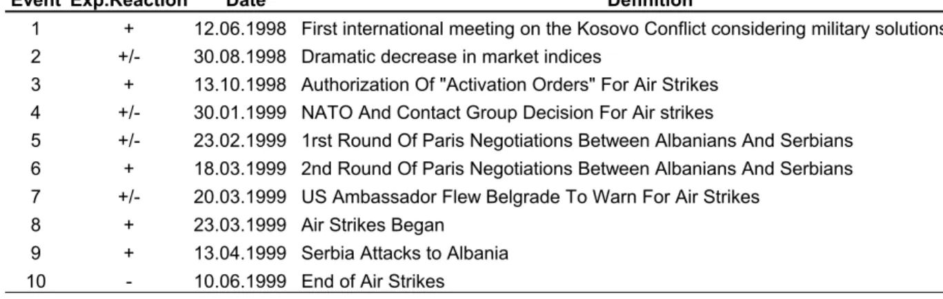
Before analyzing the statistical tests, Figure 1 presents CARs for the overall sample in order to give some feeling about the data.
Figure 1 shows the CARs beginning from 20 days before the first event in Table 5 (12 June 1998, the first international meeting on the Kosovo conflict), which is taken as day 0. In Figure 1, it can be seen that there is a downward trend in the CARs of defense stocks. After the end of Cold War, stocks of defense companies have not soared for more than a decade.14 There were a clearly defined enemy and high spending on defense fuelled by the Cold War on those days. Now the U.S. and European armies have fewer personnel and defense budgets have shrunk by 100 billion dollars. As a result of this, the downward trend has been observed since the end of the Cold War.11
Figure 1
CARs of All Firms Portfolio
-0.1800 -0.1600 -0.1400 -0.1200 -0.1000 -0.0800 -0.0600 -0.0400 -0.0200 0.0000 0.0200 -20 -6 8 22 36 50 64 78 92 106 120 134 148 162 176 190 204 218 232 246 260 274 288 302 316 330 344 358 372 386 400 414 Days CA Rs (% )