Inflation risk and default risk in a dynamic general equilibrium asset pricing model for an emerging market economy

INFLATION RISK AND DEFAULT RISK

IN A DYNAMIC GENERAL EQUILIBRIUM

ASSET PRICING MODEL

FOR AN EMERGING MARKET ECONOMY

A Master’s Thesis by

M. FATİH EKİNCİ

Department of Economics Bilkent University Ankara September -2002

I certify that I have read this thesis and have found that it is fully adequate, in scope and quality, as a thesis for the degree of Master of Arts in Economics.

--- Assistant Professor Dr. Erdem Başçõ Supervisor

I certify that I have read this thesis and have found that it is fully adequate, in scope and quality, as a thesis for the degree of Master of Arts in Economics.

--- Associate Professor Dr. Farhad Husseinov Examining Committee Member

I certify that I have read this thesis and have found that it is fully adequate, in scope and quality, as a thesis for the degree of Master of Arts in Economics

--- Assistant Professor Dr. Levent Akdeniz

Examining Committee Member

Approval of the Institute of Economics and Social Sciences

--- Professor Dr. Kürşat Aydoğan Director of Institute of Economics and Social Sciences

ABSTRACT

“Inflation Risk and Default Risk in a Dynamic General

Equilibrium Asset Pricing Model for an Emerging Market Economy”

Ekinci, Mehmet Fatih

M.A., Department of Economics Supervisor: Assistant Prof. Erdem Başçõ

September 2002

In this thesis, the difference between the T-Bill returns and common stock returns in Turkey is examined. It is observed that there is a bond premium in Turkey unlike the equity premium observed in developed countries. To understand this surprising observation, inflation-risk and default-risk are incorporated to the Mehra-Presscott (1985) dynamic asset pricing model. Inflation-risk alone is found to be insufficient to explain this bond premium. Only after allowing for a perceived default-risk, the observed bond premium of Turkish T-Bills over Turkish common stocks can be explained by such a model.

Keywords: Equity Premium Puzzle, Default Risk, Inflation Risk, Asset Pricing, Bond Premium.

ÖZET

Gelişmekte olan bir Piyasa Ekonomisi için Dinamik bir Genel Denge Varlõk Fiyatlandõrma Modelinde Enflasyon ve Default Riski

Ekinci, Mehmet Fatih Master, İktisat Bölümü Tez Yöneticisi: Yrd. Doç. Dr. Erdem Başçõ

Eylül, 2002

Bu tez, Türkiye’deki hazine tahvili getirileri ve borsa getirileri arasõndaki fark üzerine bir çalõşmadõr. Türkiye’de gelişmiş ülkelerdeki hisse primlerinin aksine bir bono primi olduğu gözlenmiştir. Bu beklenmeyen tespit üzerine Mehra-Presscott (1985) dinamik varlõk fiyatlandõrma modeline enflasyon riski ve default riski uygulanmõştõr. Enflasyon riskinin bu bono primini açõklamakta yetersiz kaldõğõ tespit edilmiştir. Ancak

default riski dahil edildiği zaman Türkiye’deki hazine tahvillerinin borsa getirilerini aşmasõ açõklanabilmiştir.

Anahtar Kelimeler: Hisse Primi Açmazõ, Default riski, Enflasyon Riski, Varlõk Fiyatlandõrma, Bono Primi.

ACKNOWLEDGEMENTS

I would like to express my deepest gratitude, first and foremost, to Assistant Professor Erdem Başçõ for his continuous support throughout this study and the support and supervision he provided during the entire course of this study. I also wish to thank

Assoc. Prof. Farhad Husseinov and Asst. Prof. Levent Akdeniz for their helpful comments.

I am truly grateful to my family for their strong encouragement during my education. I am also indebted to my colleagues at the State Planning Organization.

TABLE OF CONTENTS

ABSTRACT iii

ÖZET iv

ACKNOWLEDGEMENTS vi

TABLE OF CONTENTS vii

LIST OF TABLES ix

LIST OF FIGURES x

1. INTRODUCTION 1

2. MODEL 6

2.1.Model with inflation risk 2.2.Model with default risk 2.3.Implications of the model

6 11 12

3. DATA 15

4. RESULTS 22

4.1. Results under inflation-risk on bonds 4.2. Results under inflation and default risk

22 23

5. CONCLUSION 26

APPENDICES APPENDIX A

LIST OF THE FIRMS IN THE STOCK INDEX

29 29

APPENDIX B

T-BILL RETURN DATA

30

APPENDIX C

COMMON STOCK INDEX LEVEL (DIVIDENDS INCLUDED)

32

APPENDIX D

TÜFE PRICE LEVEL

LIST OF TABLES

Table Page

3.1 Geometric averages of the data series. 20

3.2 Covariances of the data series. 20

3.3 Correlation coefficients of the data series. 20

4.1 Model Parameters that produce the historically observed values of real stock returns and the real interest rate on T-Bills.

LIST OF FIGURES

Figure Page

3.1 Real Stock Returns calculated from ISE100 index and the index (RSR) generated with selected stocks.

16

3.2 Real annual consumption growth calculated with the SIS data. 18

3.3 Annual inflation in the sample period. 19

4.1 The points which are theoretically possible under only inflation-risk on the real interest rate-equity premium plane.

SECTION 1 : INTRODUCTION

The difference between the average return on common stocks (a risky asset) and the average return on govenrment securities (Treasury bills, T-bills) is called “equity premium”. Possible reasons for this difference is first disscussed by Mehra and Presscott (1985) in a dynamic general equilibrium model. A variation of Lucas’ (1978) asset pricing model is used by Mehra and Presscott. This theoretical model, when calibrated with US data, can produce a maximum of 0.4 percent equity premium, which is very far from the historically observed equity premium in US data,1 namely 6.18 percent over the 1889-1978 period. This unexplained excess return from common stocks is called “Equity Premium Puzzle” . This premium is even more pronounced over the post-war period as 7.8 percent in the 1947-2000 period.2 The finding of significantly high excess return on common stocks is not unique to US economy. Campbell (1999) also reports equity premium puzzles for Australia, Canada, France, Germany, Italy, Japan, the Netherlands, Sweden, Switzerland, the United Kingdom. Since these countries account for more than 85% of the capitalized global equity value, the puzzle can not be overlooked easily.

There have been many attemps to resolve the puzzle over the past 17 years.3 Two main methods are proposed in these attemps. First is to impose modifications in the utility function. Campbell and Cochrane (1999) use a habit formation utility function in the model. Another approach is to model the investors’ risk aversion as asymmetric between gains and losses. Ang, Bekaert and Liu (2001) uses the disappointment aversion

1

Mehra and Presscott(1985).

2

Siegel (1998).

3

utility approach of Gül (1991), and Benartzi and Thaler (1995) proposes the mypoic loss aversion utility which are typical examples of these attempts. Second is to use market imperfections, transaction costs and investor heterogeneity to address the puzzle. Fischer (1994) imposes transaction costs to the Mehra-Presscott model and an equity premium in the order of 3-4 percent is generated with the plausible values of the transaction cost parameters. Telmer (1993) modifies the model to incorporate heterogeneous agents and incomplete markets. Ebrahim and Mathur (2001) model investor heterogeneity, market segmentation and optimal leverage (with complete markets, ignoring the transaction costs). Thereby, they investigate the puzzle without a preference modification.

This thesis is the first attemp to explore the presence or absence of equity premium puzzle in the Turkish Capital Market. But the model of Mehra and Presscott is not directly applicable with Turkish data. In Mehra and Presscott (1985) inflation-risk on real T-bill returns are ignored. However due to the high and volatile inflation in Turkey, it may not be appropriate to set this risk to zero a priori. The Mehra and Prescott (1985) assumption can alternatively be stated as zero correlation between unanticipated inflation and the real growth rate of consumption. A close examination of the Turkish data reveals that this assumption is not valid for the case of Turkey.4 Therefore the same model is not applicable for a study in a high-inflation country like Turkey. Since the asset pricing model must include inflation risk components, the model is restated in nominal terms. As a result of this modification, the model is capable of explaining the inflation risk on bonds and as well as that on stocks.

4

Bonds obviously do not provide any hedge against surprise inflation. In contrast, the classical Fischer model implies that stocks provide a hedge against inflation 5. Stocks provide a hedge against inflation when investors are completely compensated for the increases in the price level through increases in nominal stock returns, thereby leaving real stock returns uneffected. In most of the literature, the estimated relation between short-term nominal stock returns and inflation is insignificant and may even be negative6. Ely and Robinson (1997) test the inflation-hedge hypothesis for 16 OECD countries, and as a result they find that stocks do not hedge against inflation in the short-run.

This fact contradicts with the classical Fischer model. This model states that real stock returns are determined by real factors independently from the rate of inflation. This contradiction is named as “stock return-inflation puzzle”. Fama (1981) explains this puzzle by a supply side explanation to this anomalous relationship. He states that in an economy with a vertical long-run supply curve, demand shocks don’t have any impact on output growth. On the other hand, the opposite is true for the supply shocks. This hypothesis states that only the component of inflation due to supply shocks will be significantly and negatively correlated with real stock returns because a favorable supply shock simultaneously reduces inflation and increases market value of firms.

Other than inflation risk, a second source of uncertainity on T-bill returns is the possibility of default on government debt. There is a vast literature on the debt dynamics and default risk. Sylla and Wallis(1998) draws attention to the US state defaults in

5

Gallagher and Taylor (2002).

6

1840s, caused by the fall in revenues. Eichengreen and Portes (1986) focuses on the interwar default experiences. Tanner (1995) examines domestic debt and financial indexation in Brazil for the 1976-1991 period. The case of Brazil in 80s is also examined by Tanner(1994), by arguing the implicit domestic default in this period.

Dooley (2000) focuses on the debt management policy for governments of developing countries. He claims that since default-risk is not relevant for the developed countries, debt management policies of developed countries can not be a useful guide for developing countries.

Drudi and Giordano (2000) argues the relationship between inflation, indexed domestic debt, and default probability. Hernandez-Trillo (1995) builds a model to estimate the probability of default with the data of 33 debtor countries. Merrick (2001) examines the implied default recovery ratio and default probability using Eurobond data of Russia and Argentina. Therefore, as a sovereign emerging market economy, Turkish government securities might not be considered by the market participants as fully default-risk free. The bond premium observed in Turkish data confirms the default-default-risk idea as well.

In this thesis, first, historical data on stock and bond returns for the 1990(1)-2002(1) period is constructed. Quite strikingly, the presence of a ‘bond premium’ is observed in the last decade of the twentieth century. Then a theoretical variant of the Mehra-Prescott (1985) dynamic asset pricing model is constructed for a high inflation

country which includes inflation-risk components. Finally, default-risk is also considered as a second variation to the model. Thereby implied default probabilities are calculated for a reasonable range of parameter values.

Organization of this thesis is as follows. Section 2 introduces the model. Section 3 gives information about the data. Section 4 presents the results of the model calibrated with Turkish data. Finally Section 5 concludes the thesis.

SECTION 2: MODEL

2.1.Model with inflation risk:

A variation of Mehra and Presscott (1985) model is used which incorporates nominal bonds to the original model. This is a representative agent model. The agent has preferences given by

[

( )

]

0 0 t t t c u W

∑

∞ = Ε = β (1)

where 0 < β < 1 and u(.) is strictly increasing, strictly concave and twice differentiable.

Agents budget constraint is given by

t t t t t t t t t t tc q b p z b p z y z g + + ₊₁ = ₋₁ + + (2)

where gt , ct , qt , bt , zt , yt , pt denote respectively price of consumption good, real consumption , nominal price of one period maturity bond at time t which is pays 1 unit of currency at time t+1, quantity of bonds purchased at time t, quantity of shares, nominal dividend received per share, and nominal price per share of the common stock. The utility of the agent is defined as typical constant relative risk aversion utility function,

σ σ − − = − 1 1 ) ( 1 c c u (3)

The interest here is to determine the competitive equilibrium prices. Consumer’s

maximization problem is t t t t t t t t t t t z b z y z p b z p b q c g to subject W t t + + = + + + − + 1 1 ,

max

1

In this maximization problem, first order conditions are

0 (.) ₌ ∂ ∂ t b W (4) 0 (.) 1 = ∂ ∂ + t z W (5)

When the first order conditions (4) and (5) are applied, expressions about the real interest rate and stock returns are obtained. The agent decides his position for the next period in the stock market and bond market at the same time as current consumption decision. By substituting consumption in the budget constraint (2) and imposing the first order

condition (4), the nominal price of bonds is obtained after some rearrangements, as of time t,       ′ ′ Ε = + + 1 1 ) ( ) ( t t t t t t g g c u c u q β (6)

Since the covariance between two random variables, x and y is given by,

[ ] [ ] [ ]

xy x y y

x, )=Ε −Ε Ε

cov( (7)

By using (4),(6) and (7), nominal price of bonds is rearranged as7,

                        +             Ε             Ε = + + + +1 1 1 1 , cov t t t t t t t t t g g c c g g c c q σ σ β (8)

Sample values of all of the expressions in the equation are computable with given time series data. If the relevant sample moments on the right hand side of equation (8) are used, the theoretical value of nominal bond price will be obtained. The implied nominal interest rate of bonds, then, is found by

1 1 ₋ = _q i , (9) 7     +1 t t g g

is equal to the gross deflation rate. It can also be expressed as

    + +1 1 1 t π where πt+1 is the

and the real interest rate of bonds can be calculated as 1 1 1 − + + = π i r (10)

where π is the is the average inflation rate over the sample period.

The second F.O.C. is related with the common stock holdings,zt+1. By substituting for consumption in equation (1) from the budget constraint (2) and applying the first order condition (5), the expression about the stock prices becomes,

      + _′ Ε = ′ ₊ + + + ) ( ) ( ₁ 1 1 1 t t t t t t t t c u g y p c u g p β (11)

After some rearrangements, equation (11) takes form,

            + Ε = + + σ β 1 1 , ) 1 ( 1 t t t s t c c r (12)

where r_s,t+1 is the real stock return8 at time t+1. If we use the covariance expansion (7), equation (12) becomes,

8 1 1 1 1 , ) 1 ( + + + + + = + t t t t t t s g g p y p r

[

]

            Ε + Ε +             + = + + + + σ σ β 1 1 , 1 1 , ), (1 ) 1 ( cov 1 t t t s t t t s c c r c c r (13)

Rearranging this equation, implied real stock returns can be expressed as,

[ ]

1 ), 1 ( cov 1 1 1 1 , 1 , −               Ε                     + − = Ε + + + + _σ σ β t t t t t s t s c c c c r r (14)

By the same method used for the calculations of the nominal interest rate on bonds, theoretical equilibrium real stock returns can be computed by using the available data.

In Mehra and Presscott (1985) the assumption which states that unanticipated inflation and the real growth rate of consumption are uncorrelated (or negligible) with the real growth rate of consumption, does not hold for Turkish data9. Therefore the same model is not applicable for a study in a high-inflation country like Turkey.

Since the asset pricing model must include inflation risk components, the model is written in nominal terms including the price level. As a result of this modification, the model is capable of explaining the inflation risk on bonds as well as on stocks.

9

2.2.Model with default risk:

Inflation is not the only possible source of risk for Turkey. Default risk may also be considered as one of the reasons for observed high real interest rates. To test the significance of this argument, a time invariant default risk can be incorporated in this model. If the budget constraint (2) is modified as

t t t t t t t t t t tc q b p z b p z y z g + + ₊₁ =ρ ₋₁ + + (2a)

where ρis a discrete and random variable,which is takes values

   − = ). 1 ( , , 1 . , , 0 d d p y probabilit with default no if p y probabilit with default if ρ Equation (6) changes as       ′ ′ Ε = + + 1 1 ) ( ) ( t t t t t t g g c u c u q β ρ (6a)

and with the assumption of independence between ρ and other random variables, nominal price for bonds10 become,

10 _{By the introduction of the random variable} ρ_{, a time invariant default risk with no recovery of face}

value is included in the model. With the assumption of independence of consumption growth rate, inflation, real stock returns, from default risk, this modification effects only the real interest rates.

                        +             Ε             Ε − = + + + +1 1 1 1 , cov ) 1 ( t t t t t t t t d t g g c c g g c c p q σ σ β (8a)

2.3.Implications of the model:

Regarding the bond prices, first, if future utility is highly discounted,which means

β is low, the nominal bond prices are low and therefore the nominal interest rates are

high.

Second, as the default probability (p ) in the model increases, nominal and real _d

price of bonds decrease, and the nominal and real interest rates increase as expected. This gives more flexibility in explaining the high real interest rates in Turkey. When p_d =0 the model reduces to the inflation-risk only model which ignores the default risk.

Third, as seen in equation (8a), nominal bond prices are discounted by the expected value of inflation, and the expected value of real consumption growth. The risk aversion parameter (σ ) is effective through the impact on real consumption growth. As the agent becomes more risk averse, which means that risk aversion parameter (σ ) is higher, this effect will be more pronounced, otherwise this effect will be smaller.

Fourth, the covariance term is also important, as it is the distinction of this model from the Mehra-Presscott model, if it is positive, which means that if the consumption growth rate is positively correlated with the inflation, the nominal bond prices will be

high. Because, in this case, bonds provide a good hedge over business cycle fluctuations. Higher nominal bond prices mean lower nominal interest rates. Otherwise, if the consumption growth rate is negatively correlated with the inflation, this effect decreases the nominal bond prices, hence leads to high nominal interest rates.

Regarding the stock prices, the subjective discount rate, β , effects real stock returns in negatively. If future utility is highly discounted, which means β is low, the equilibrium real stock returns are high.

Second, as seen in equation (14), real stock returns are positively related with the expected value of future real consumption growth. The risk aversion parameter (σ ) is effective on the impact of real consumption growth. As the agent becomes more risk averse, which means that risk aversion parameter (σ ) is higher, this effect will be more pronounced, otherwise this effect will be smaller.

Third, the covariance term between the real stock returns and the inverse of the real consumption growth is effective, if it is positive, which means that if the consumption growth rate is negatively correlated with the real stock returns, mean value of the real stock returns decrease. Otherwise, if the consumption growth rate is positively correlated with the real stock returns, which means the covariance term in the equation is negative, equilibrium real stock returns increase.

Comovements of the macroeconomic variables in the model have strong effects on the interest rates and the real stock returns as well. These findings lead us to question whether stock market is a good hedge over the business cycle fluctuations. If the real stock returns have a positive correlation with the consumption growth, stock market is not a good hedge for bad times over the business cycle. To be a good hedge for the fluctuations, stock holdings should give higher returns in the periods during which the consumption growth is low or negative. The covariance term in the equation (14) implies that if stock holdings are a not a good hedge for fluctuations then equilibrium expected stock returns will be high since the stock prices will be discounted heavily by the market.

SECTION 3: DATA

Consumption, stock returns, inflation and T-bill returns are the necessary data series to obtain empirical results from the model. Since the number of observations is limited, instead of yearly data, quarterly data is used in this thesis. To find meaningful results with quarterly data, seasonal effects must be eliminated. The traditional filtering mechanisms like HP filter cause loss of valuable information, so the same quarter in the following year is used as the next period in the model. This method, known as seasonal differencing, does not cause loss of information and the strong seasonality in consumption data is safely eliminated.

The demise of restrictions on capital movements in 1989 has an important effect on the asset prices in Turkey. Since this is an important structural change in Turkish economy, data sample starting with the first quarter of 1990, and ending with the first quarter of 2002 is used.

Historical values of bond returns and the stock returns are the key variables for the empirical test of the model. Bond returns are calculated from the treasury auctions series. The method for constructing T-bill returns is to simulate a representative agent who purchases bonds from the treasury auctions and keeps reinvesting the principal and the interest obtained. To find the bond returns, series of treasury auctions11 is obtained from the electronic database of the Central Bank of the Republic of Turkey. In order to

11

keep the average maturity as close to three months (a quarter) as possible, the auctions of three months maturity are picked whenever available. If not, the auctions closest to three months maturity are picked. The gaps in timing are filled with data from Istanbul Stock Exchange (ISE) secondary bond market and overnight repo market of ISE. After this exercise, the geometric average of annual real bond returns is found as 14.12 percent where nominal returns are deflated by TÜFE12.

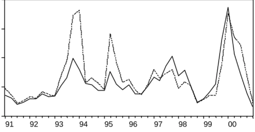
-100 0 100 200 300 91 92 93 94 95 96 97 98 99 00 ISE100 RSR

On the other hand, real stock returns from ISE can be calculated as

4 4 100 , 4 + + + − = t t t t t ISE t g g ISE ISE ISE r (1)

where ISE is the nominal level of ISE-100, _t g is the TÜFE (CPI) price level and _t r_t,ISE−100

is the real return of ISE-100 at time t. Quarterly nominal level of ISE-100 is found by taking the arithmetic average of the ISE-100 index at the end of the days in the quarter.

12

TÜFE is the Consumer Price Index of State Institute of Statistics.

Figure 3.1. Real Stock Returns calculated from ISE100 index and the index (RSR) generated with selected stocks. Returns are deflated with the TÜFE price level.

ISE composite market index does not include the dividend payments, it only gives an idea about price level of stocks. The ISE index is adjusted for stock splits and rights offerings but not for dividends. Therefore the composite index of ISE is not reflecting the returns of a representative stockholder. The geometric average annual real returns of ISE-100 index is found as -4.80 percent during the sample period. Since the dividend payments are not included in this index, another index which includes the dividend payments is constructed and used since it is more reasonable to simulate a representative agent’s stock returns by taking dividends into consideration.

In constructing the index, the stockholders are assumed to reinvest in the same stocks when they receive a dividend from a particular stock. A total of 25 firms13 are chosen which have been continuously traded in the stock market during the whole period between the foundation of the stock market (January 1986) and today (April 2002). The agent is assumed to carry an equally weighted portfolio of these 25 firms14. A nominal dividend inclusive monthly stock price index is computed with this assumption. By taking the geometric average of this monthly index, a quarterly series15 for this new stock index is computed. Real returns from the index generated is calculated as

4 4 4 + + + − = t t t t t t g g P P P r (2) 13

The list of these firms are available in Appendix A.

14

Monthly portfolio rebalancing to preserve equally weights is assumed.

15

where P is the level of nominal index generated, _t g is the TÜFE (CPI) price level and _t r _t

is the real returns of the generated index at time t.

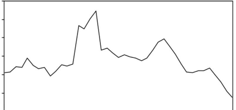
From this index, annual geometric average nominal stock return in Turkey is calculated as 90.96 percent in the sample period. After adjusting for inflation, the geometric annual average real stock return in Turkey is found to be 9.84 percent in the sample period. -15 -10 -5 0 5 10 15 91 92 93 94 95 96 97 98 99 00

Consumption data is taken from the State Institute of Statistics (SIS). Both annual and quarterly consumption series are reported by SIS. Quarterly data, which is more suitable for our purposes is chosen in this study. The model requires the use of the real consumption, therefore the series of private consumption at fixed prices (1987) is taken.

Consumption growth is calculated as

t t t t C C C cg ₊ = +4− 4 (3)

Figure 3.2. Real annual consumption growth calculated with the SIS data. Quarterly private consumption at fixed prices (1987) series is used.

where C is the consumption, _t cg is the consumption growth at time t. Annual geometric _t

average of consumption growth is 3.36 percent during the sample period.

20 40 60 80 100 120 140 91 92 93 94 95 96 97 98 99 00

Monthly reported Consumer Price Index (1987=100) of SIS is used to calculate an appropriate quarterly inflation series. Since this monthly price index is reflecting the average level of prices collected at various instances in a month16, geometric average of the three months in every quarter is calculated to find an appropriate price index 17for the quarter. Inflation is calculated as

t t t t g g g − = + +4 4 π (4) 16

Urban Places Consumer Price Index Concepts, Methods and Sources (1987=100) , State Intitute of Statistics Prime Ministry Of Turkey.

17

This series is available in Appendix D.

Figure 3.3. Annual inflation in the sample period. Consumer Price Index (TÜFE) of SIS is used to calculate inflation data.

where π is the inflation, _t g is the TÜFE (CPI) price level at time t. Annual average _t

inflation rate is found to be 73.86 percent during the same period.

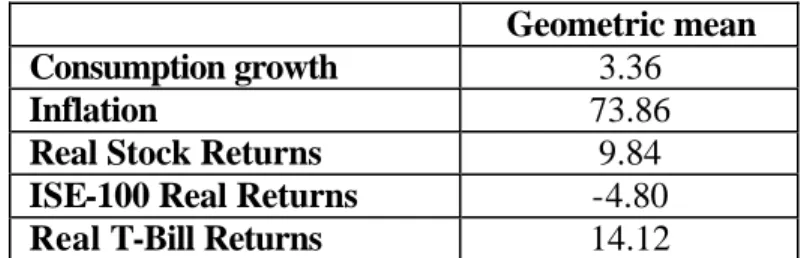
Table 3.1. Geometric averages of the data series. Geometric mean

Consumption growth 3.36

Inflation 73.86

Real Stock Returns 9.84

ISE-100 Real Returns -4.80 Real T-Bill Returns 14.12

The average values of the consumption growth, T-bill interest rates, inflation and real stock returns are computed as geometric averages to be compatible with their theoretical counterparts in the model.

Table 3.2. Covariances of the data series.18

cg rsr inf uinf

cg 0.0032 0.0183 -0.0035 -0.0029

rsr 0.0183 0.7087 -0.0038 -0.0016

inf -0.0035 -0.0038 0.0354 0.0343

uinf -0.0029 -0.0016 0.0343 0.0343

Table 3.3. Correlation coefficients of the data series.

cg rsr inf uinf cg 1 0.3822 -0.3152 -0.2815 rsr 0.3822 1 -0.0244 -0.0099 inf -0.3152 -0.0244 1 0.9852 uinf -0.2815 -0.0099 0.9852 1 18 cg : Consumption Growth. inf : Inflation.

uinf : Unanticipated Inflation. rsr : Real Stock Returns.

The covariance statistics of the series are reported in Table 3.2 and the correlations between the series are reported in Table 3.3. The main purpose is to investigate the validity of the assumption of uncorrelatedness of consumption growth and unanticipated inflation made by Mehra-Presscott (1985) The unanticipated inflation seen in the tables is obtained from the residual series of the regression of current annual inflation on the last year’s annual inflation. The correlation between consumption growth and unanticipated inflation is -0.2815. In bad years for consumption, inflation tends to be unexpectedly high and vice versa. It is obvious that the Mehra-Presscott assumption of uncorrelatedness does not hold with Turkish data. Therefore, bonds are not a good hedge against business cycle fluctuations. Also, the positive correlation between the real stock returns and consumption growth supports that stocks do not provide a good hedge against business cycle fluctuations in Turkey.

SECTION 4 : RESULTS

4.1. Results Under Inflation-Risk on Bonds :

First,the results of the model are studied by taking default risk as zero (ρ=0). Thereby, the possibility of producing the historically observed negative equity premium is investigated by changing β∈

[ ]

0,1 and σ∈

[ ]

0,10 . The admissible region for equity premium and real T-Bill interest rate seen in the Figure 4.1 is obtained by using the model parameters in these intervals. Since the historically observed average real interest rate on Turkish T-Bills is 14.12 percent and the average real stock returns is 9.84 percent, observed equity premium in the sample period turns out to be –4.28 percent. Point H shows these historically observed values as a point on the real interest rate-equity premium plane.

Figure 4.1. The points which are theoretically possible under only inflation-risk on the real interest rate-equity premium plane. Point H shows the historically returns.

When σ=0, representative agent has a linear utility function which corresponds to the risk neutral case. Equity premium becomes zero in this situation, since stocks and T-Bills are perfect substitutes under risk neutrality. Therefore these values form a lower-bound for the equity premium in the admissible region. When the curvature of the utility function is increased (as σ increases), the agent becomes more risk averse. This increases the equity premium. In this model, it also increases the real interest rate on T-Bills, since T-Bills are subject to inflation-risk. In contrast Mehra and Presscott ignores the inflation-risk on T-Bills, therefore in their version the value of β alone determines the risk-free interest rate. Under inflation-risk on T-Bills, as β decreases, real interest rate increases and the iso-beta line shifts to right as seen in Figure 4.1.

As seen in the figure, the model with only inflation-risk on T-Bills can not produce a negative equity premium, so it is not capable of explaining the historically observed negative value of the equity premium in Turkish data19.

4.2. Results under inflation and default risk :

As a sovereign emerging market economy,Turkish government securities might not be considered as fully default-risk free. There has been considerable discussion in the Turkish press on the possibility of “consolidation” during the 90’s. This also indicates the possibility of a perceived default-risk on Turkish T-Bills by the market participants.

19

Although negative equity premium observed in Turkish economy is not possible according to this covariance structure, it may be worth while exploring inflation-risk on bonds to adress the equity premium puzzle in US economy.

In this study, the default probability considered is the implied probability of a zero-recovery default. The investors who have purchased T-Bills are assumed to lose the amount they invested. The default-risk values in Table 4.1 are the probability of a zero-recovery default. These are calculated by equation (8a) in Section 2. Also it is possible to do this work with a partial-recovery assumption. If a partial-recovery default probability were investigated, the implied probability of default turn out to be higher than these values.

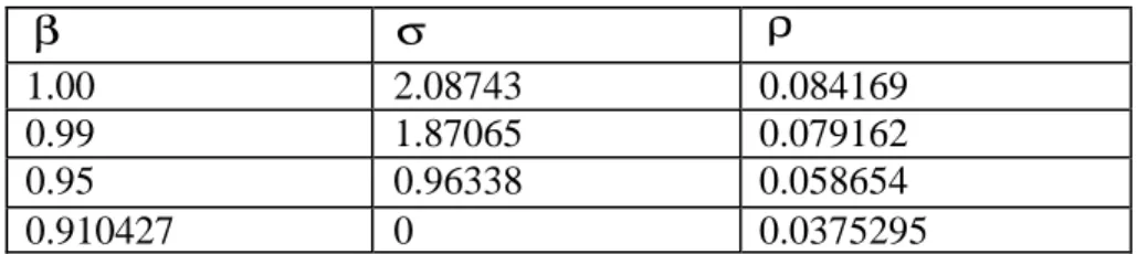
In Table 4.1, the value of β is fixed and the value of σ is calibrated so as to match the historically observed value of the real stock returns. After this procedure, the value of the real interest rate on T-Bills is calibrated with the default probability. By this method, the values of ρ and σ are obtained which match historically observed real stock returns and real interest rate on T-Bills for a given β .

β σ ρ

1.00 2.08743 0.084169

0.99 1.87065 0.079162

0.95 0.96338 0.058654

0.910427 0 0.0375295

The values of the model parameters with selected subjective discount rates which explains this bond premium are seen in the Table 4.1. The minimum possible β is

Table 4.1. Model Parameters that produce the historically observed values of real stock returns and the real interest rate on T-Bills.

0.910427 to obtain the historically observed real stock returns from the model. This corresponds also to the minimum default probability to explain the bond premium observed. The average default probability changes from 3.75 percent to 8.42 percent depending on the chosen value of β . After this emprical analysis, it is obvious that inflation-risk is not sufficient to explain the bond premium. The model is not able to explain the negative equity premium in Turkish economy without allowing the presence of a perceived default risk of about 4 to 8 percent in probability.

SECTION 5 : CONCLUSION

In this thesis, an asset pricing model for a high inflation emerging economy is constructed. By this model, Turkish bond premium observed during the 1990-2001 period is examined. Allowing for inflation-risk on bonds and stocks is considered as a first contribution to the Mehra-Presscott model. Default-risk is also introduced as a second variation to the model. A zero-recovery default is assumed when default-risk calculations are made.

Calibration results for Turkey are obtained with inflation-risk and default-risk possibilities allowed for. Inflation-risk is found to be insufficient to explain the negative equity premium observed in Turkish data. Imposing a default-risk, however, brings a theoretical explanation to the Turkish bond premium.

As further work, the situation in other emerging market economies may be investigated. Perceived default-risk in these countries may be examined by the model developed here. Also the neglected inflation-risk in the Mehra-Presscott model seems to be promising to adress the equity premium puzzle in the US and other developed economies. Another promising line of research is, by means of some modifications to the model, to obtain the time-varying perceived default default probabilities in emerging markets. Also a more reasonable recovery rate assumption may be imposed by using the historical default experiences.

BIBLIOGRAPHY

Ang A., Bekaert G. and Liu J., “Why Stocks May Disappoint”, 2000, NBER Working Paper 7783.

Benartzi and Thaler, 1995, “Myopic Loss Aversion and the Equity Premium Puzzle”, Quarterly Journal of Economics, 110 : 73-92.

Campbell, J. Y. (1999), “ Asset Prices, Consumption and the Business Cycle “, Handbook of Macroeconomics, vol.IC.

Campbell, J. Y. , Cochrane, J. H. (1999), “By Force of Habit: A Consumption-Based Explanation of Aggregate Stock Market Behaviour”, The Journal of Political Economy, 107: 205-251.

Dooley, M. P.,2000, “Debt management and crisis in developing countries”, Journal of Development Economics, 63 : 45-58.

Drudi, F., Giordano, R., 2000, “Default Risk and Optimal Debt Management”, Journal of Banking and Finance, 24: 861-891.

Ebrahim, M. S. and Mathur , I. , 2001, “Investor Heterogeneity, Market Segmentation, Leverage and the Equity Premium Puzzle”, Journal of Banking and Finance, 25 : 1897-1919.

Eichengreen, B., Portes, R., 1986, “Debt and Default in the 1930s: Causes and Consequences”, European Economic Review, 30 : 599-640.

Ely, D.P. and K.J. Robinson, 1997, “Are Stocks Hedge Against Inflation,International Evidence Using a Long-Run Approach”, Journal of International Money and Finance, 16 : 141-167.

Fama E. F. , 1981, “Stock Returns,Real Activity,Inflation,and Money”, American Economic Review, 71 : 545-565.

Fama, E.F. and Schwert, G. W. (1977),”Asset returns and Inflation”, Journal of Financial Economics, 5 : 115-146.

Fischer, S.J., 1994, “Asset Trading,Transaction Costs and the Equity Premium”, Journal of Applied Econometrics, 9 : 71-94.

Gül F., 1991, “A Theory of Disappointment Aversion”, Econometrica, 59: 667-686. Gültekin, N. B. , “Stock Market Returns and Inflation: Evidence from other countries”, Journal of Finance 38 : 49-65.

Kocherlakota, N. , 1996, “The Equity Premium: It is Still a Puzzle”, Journal of Economic Literature, 42-71.

Gallagher L. A., Taylor M. P., “The stock return-inflation puzzle revisited”, Economics Letters, 75 : 147-156.

Hernandez-Trillo, F., 1995, “A model-based estimation of the probability of default in sovereign credit markets”, Journal of Development Economics, 46 : 163-179.

Lucas , R. E. Jr. , 1978, “Asset Prices in an Exchange Economy”, Econometrica 46 : 1429-1445.

Mehra, R. and Presscott, E. C. , 1985, “The Equity Premium: A Puzzle”, Journal of Monetary Economics, 15 : 145-161, .

Mehra, R., 2001, “The Equity Premium Puzzle”, University of California, Santa Barbara, manuscript, http://www.econ.ucsb.edu/~mehra.

Merrick Jr., J. J., 2001, “Crisis Dynamics of Implied Default Recovery Ratios: Evidence from Russia and Argentina”, Journal of Banking and Finance, 25 : 1921-1939. Siegel, J., 1998, Stocks for the Long Run. (2nd edition). New York. Irwin.

Sylla, R., Wallis, J. J., 1998, “The anatomy of sovereign debt crises: Lessons from the American state defaults of the 1840s”, Japan and the World Economy, 10 : 267-293. Tanner, E., 1994, “Balancing the Budget with Implicit Domestic Default: The Case of Brazil in the 1980s”, World Development, 22 : 85-98.

Tanner, E., 1995, “Intertemporal solvency and indexed debt: evidence from Brazil,1976-1991”, Journal of International Money and Finance, 14 : 549-573.

Telmer, C. , 1993, “Asset-Pricing Puzzles and Incomplete Markets”, Journal of Finance, 48 : 1803-1832.

Urban Places Consumer Price Index (1987=100), 1987, State Institute Of Statistics (Prime Ministry Of Republic Of Turkey) Publications.

APPENDIX A

LIST OF THE FIRMS IN THE STOCK INDEX

ANADOLU CAM ARÇELİK BAGFAŞ BRİSA ÇELİK HALAT ÇİMSA DÖKTAŞ ECZACIBAŞI YATIRIM EGE GÜBRE

EREĞLİ DEMİR ÇELİK FORD OTOSAN GÜBRE FABRİKALARI HEKTAŞ İZMİR DEMİR ÇELİK İZOCAM KARTONSAN KAV KOÇ HOLDİNG KORDSA OLMUKSA PİMAŞ PİRELLİ KABLO(SİEMENS) SARKUYSAN ŞİŞECAM T. DEMİR DÖKÜM

APPENDIX B

T-BILL RETURN DATA USED

(TREASURY AUCTIONS AND REPOS

TO FILL THE GAPS WHEN NEEDED)

Auction No. Auctions Date Issue Date Maturity Date Days to Maturity

Annualized Simple Interest Rate

452 13-Dec-89 20-Dec-89 21-Mar-90 91 40.76

464 07-Mar-90 14-Mar-90 13-Jun-90 91 40.56

476 30-May-90 06-Jun-90 05-Sep-90 91 40.88

487 22-Aug-90 29-Aug-90 28-Nov-90 91 45.84

499 14-Nov-90 21-Nov-90 20-Feb-91 91 50.36

511 06-Feb-91 13-Feb-91 15-May-91 91 59.60

523 01-May-91 08-May-91 07-Aug-91 91 71.44

535 24-Jul-91 31-Jul-91 30-Oct-91 91 67.60

547 16-Oct-91 23-Oct-91 22-Jan-92 91 72.36

559 08-Jan-92 15-Jan-92 15-Apr-92 91 67.72

571 01-Apr-92 08-Apr-92 08-Jul-92 91 68.44

583 24-Jun-92 01-Jul-92 30-Sep-92 91 76.88

595 16-Sep-92 23-Sep-92 23-Dec-92 91 74.40

607 09-Dec-92 16-Dec-92 17-Mar-93 91 74.76

619 03-Mar-93 10-Mar-93 09-Jun-93 91 65.32

633 26-May-93 31-May-93 01-Sep-93 93 67.12

645 18-Aug-93 25-Aug-93 24-Nov-93 91 65.76

653 13-Oct-93 20-Oct-93 19-Jan-94 91 63.04

REPO 19-Jan-94 24-Jan-94 5

668 19-Jan-94 24-Jan-94 11-May-94 107 75.49

692 03-May-94 04-May-94 03-Aug-94 91 130.00

730 21-Jul-94 03-Aug-94 02-Nov-94 89 100.08

764 31-Oct-94 02-Nov-94 01-Feb-95 89 82.28

784 25-Jan-95 26-Jan-95 27-Apr-95 91 108.08

801 26-Apr-95 27-Apr-95 27-Jul-95 90 77.36

REPO 27-Jul-95 04-Aug-95 7

813 02-Aug-95 04-Aug-95 03-Nov-95 89 66.96

REPO 03-Nov-95 09-Nov-95 6

828 08-Nov-95 09-Nov-95 29-Jan-96 80 92.52

840 24-Jan-96 25-Jan-96 08-May-96 103 112.00

854 07-May-96 08-May-96 06-Nov-96 178 97.42

876 05-Nov-96 06-Nov-96 06-Aug-97 270 94.79

REPO 06-Aug-97 20-Aug-97 14

904 18-Aug-97 20-Aug-97 10-Dec-97 110 78.36

913 09-Dec-97 10-Dec-97 18-Mar-98 98 89.25

922 17-Mar-98 18-Mar-98 17-Jun-98 89 83.28

930 02-Jun-98 04-Jun-98 02-Dec-98 178 75.98

952 08-Dec-98 09-Dec-98 21-Jul-99 222 121.71

REPO 21-Jul-99 28-Jul-99 7

986 26-Jul-99 28-Jul-99 27-Oct-99 89 75.06

996 05-Oct-99 06-Oct-99 24-May-00 228 89.68

1018 15-May-00 17-May-00 16-Aug-00 89 35.02

1026 14-Aug-00 16-Aug-00 15-Nov-00 89 28.24

1034 13-Nov-00 15-Nov-00 14-Feb-01 89 35.20

1042 13-Feb-01 14-Feb-01 16-May-01 92 57.03

APPENDIX C

COMMON STOCK INDEX LEVEL

(DIVIDENDS INCLUDED)

COMMON STOCK INDEX LEVEL (1.1.1990=100)

1990Q1 138.27 1990Q2 182.36 1990Q3 249.72 1990Q4 200.44 1991Q1 214.17 1991Q2 215.28 1991Q3 187.71 1991Q4 177.80 1992Q1 256.93 1992Q2 226.12 1992Q3 259.55 1992Q4 224.48 1993Q1 275.12 1993Q2 501.39 1993Q3 854.70 1993Q4 1320.89 1994Q1 1716.85 1994Q2 1239.17 1994Q3 2345.23 1994Q4 3319.31 1995Q1 3604.48 1995Q2 6567.55 1995Q3 8036.77 1995Q4 7038.69 1996Q1 8101.99 1996Q2 10665.37 1996Q3 10693.98 1996Q4 13250.08 1997Q1 22750.21 1997Q2 24532.15 1997Q3 29481.26 1997Q4 41375.70 1998Q1 43261.06 1998Q2 55227.36 1998Q3 55421.72 1998Q4 32219.20

1999Q1 39957.07 1999Q2 63178.65 1999Q3 64445.75 1999Q4 95720.64 2000Q1 235981.93 2000Q2 274584.87 2000Q3 240813.33 2000Q4 194376.38 2001Q1 144809.19 2001Q2 167455.43 2001Q3 173868.22 2001Q4 161868.73 2002Q1 222146.67

APPENDIX D

TÜFE PRICE LEVEL

CONSUMER PRICE INDEX (TÜFE) LEVEL (1.1.1987=100) 1990Q1 378.92 1990Q2 434.89 1990Q3 459.53 1990Q4 543.85 1991Q1 616.13 1991Q2 709.54 1991Q3 775.67 1991Q4 914.43 1992Q1 1098.81 1992Q2 1205.15 1992Q3 1290.20 1992Q4 1535.41 1993Q1 1743.20 1993Q2 1972.91 1993Q3 2204.22 1993Q4 2599.30 1994Q1 2999.64 1994Q2 4215.12 1994Q3 4617.94 1994Q4 5730.48 1995Q1 6882.01 1995Q2 7880.44 1995Q3 8737.18 1995Q4 10523.21 1996Q1 12313.28 1996Q2 14299.67 1996Q3 15717.65 1996Q4 18713.14 1997Q1 21586.07 1997Q2 25455.58 1997Q3 29306.63 1997Q4 36536.66 1998Q1 42974.08 1998Q2 48380.00 1998Q3 53368.22 1998Q4 62635.77

1999Q1 69942.54 1999Q2 78473.66 1999Q3 87639.61 1999Q4 102934.10 2000Q1 117017.90 2000Q2 125896.90 2000Q3 133485.70 2000Q4 146684.90 2001Q1 158801.40 2001Q2 191045.10 2001Q3 210430.80 2001Q4 244675.00 2002Q1 269841.30