MAXIMIZING PROFIT PER UNIT TIME IN
COINTEGRATION BASED PAIRS TRADING
A THESIS
SUBMITTED TO THE DEPARTMENT OF INDUSTRIAL ENGINEERING
AND THE GRADUATE SCHOOL OF ENGINEERING AND SCIENCE OF BILKENT UNIVERSITY
IN PARTIAL FULFILLMENT OF THE REQUIREMENTS FOR THE DEGREE OF
MASTER OF SCIENCE
by Duygu Tutal January, 2014
ii
I certify that I have read this thesis and that in my opinion it is full adequate, in scope and in quality, as a dissertation for the degree of Master of Science.
___________________________________ Assoc. Prof. Savaş Dayanık (Advisor)
I certify that I have read this thesis and that in my opinion it is full adequate, in scope and in quality, as a dissertation for the degree of Master of Science.
___________________________________ Assoc. Prof. Sinan Gezici
I certify that I have read this thesis and that in my opinion it is full adequate, in scope and in quality, as a dissertation for the degree of Master of Science.
______________________________________ Asst. Prof. Emre Nadar
Approved for the Graduate School of Engineering and Science
____________________________________ Prof. Dr. Levent Onural
iii
ABSTRACT
MAXIMIZING PROFIT PER UNIT TIME IN COINTEGRATION BASED PAIRS TRADING
Duygu Tutal
M.S. in Industrial Engineering Advisor: Assoc. Prof Savaş Dayanık
January, 2014
Pairs Trading is a modest but persistent statistical arbitrage strategy. It is based on identifying a pair of stocks whose prices are driven by the same economic forces, and trade according to the spread between their prices. In this thesis, we study on a pairs trading method which maximizes the profit per unit time. We identify the pairs using cointegration analysis and build the method using Markov Chains. After constructing the method, we examine its performance on both simulated and real data. We use banking stocks from Istanbul Stock Exchange as real data.
iv
ÖZET
BİRİM ZAMANDAKİ KARI MAKSİMUMA ULAŞTIRAN EŞBÜTÜNLEŞME BAZLI EŞLİ ALIM-SATIM METODU
Duygu Tutal
Endüstri Mühendisliği, Yüksek Lisans Tez Yöneticisi: Doç. Dr. Savaş Dayanık
Ocak, 2014
Eşli Alım-Satım tekniği az miktarda ama devamlı kar sağlayan bir istatistiksel arbitraj yöntemidir. Bu metod, fiyatları aynı ekonomik sebeplerden etkilenen bir çift hisse senedi belirleyip, bu iki hisse senedinin fiyatları arasındaki farka göre alım-satım yapmaya dayanır. Bu tezde birim zamandaki karı maksimize etmeye dayanan bir eşli alım-satım metodu üzerinde çalışılmıştır. Hisse senedi çiftleri eşbütünleşme yöntemi kullanılarak belirlenmiş ve metod Markov Zinciri’nin özelliklerinden faydalanılarak oluşturulmuştur. Çalışmanın sonunda metod, hem simüle edilmiş, hem de gerçek veriler üzerinde denenerek metodun performansı ölçülmüştür. Gerçek veri olarak Borsa İstanbul’un bankacılık hisse senetleri kullanılmıştır.
Anahtar Sözcükler: Eşli Alım-Satım, Eşbütünleşme, Zaman Serileri Analizi, Markov Zinciri.
v
vi
ACKNOWLEDGEMENT
First and foremost, I would like to express my gratitude to my advisor, Assoc. Prof. Savaş Dayanık.
I would like to thank the members of my thesis committee Assoc. Prof. Sinan Gezici and Asst. Prof. Emre Nadar for critical reading of this thesis and for their valuable comments.
I am grateful to my precious friend Ezel Ezgi Budak Ayar for being such a long time in my life. I feel she is always there for me with her great heart and endless support. This thesis would not be possible without her help, patience and support. I also wish to thank Müge Güçlü, Burak Ayar and Mustafa Karakul for their academic assistances. I am also indeed grateful to Fatih Cebeci for his encouragement, patience and support. I am also thankful to Nur Budak and Özcan Budak for their great support. I am also grateful to all other friends that I failed to mention here.
Last but not the least; I also would like to express my deepest gratitude to my mother Yurdagül Tutal, father Mustafa Tutal, and sister Beste Tutal for their eternal love, support and trust at all stages of my life and especially during my graduate study.
vii
Contents
1. Introduction ... ..1
2. Literature Review... 5
2.1 Cointegration-based Strategies ... 5
2.2 Pairs Trading and Statistical Arbitrage Studies ... 6
3. Problem Definition ... 10
3.1 Maximizing Profit per Unit Time in Pairs Trading ... 10
3.2 Cointegration ... 12
4. Proposed Pairs Trading Method ... 14
5. Case Study ... 20
5.1 Stock Price Data from BIST ... 20
5.2 Profit per Unit Time for 𝑋0 = 0 ... 32
5.3 Profit per Unit Time for a Random Starting Point ... 34
6. Numerical Results ... 41
6.1 Performance Measurement Using Simulated Data ... 41
viii
6.3 Performance Measurement Using BIST Banking Stock Data ... 50
7. Conclusion and Future Research ... 54
Bibliography ... 57
Appendix A: Time Series Plots of the Banking Stock Pairs ... 60
Appendix B: Model Outputs of the Cointegration Equations…………....….68
Appendix C: Profit per Unit Time Graphs for X0 = 0….………...72
Appendix D: Density, Empirical CDF and Q-Q Plots of Starting Points...75
Appendix E: Expected Profit per Unit Time for Random Starting Point..88
Appendix F: Profit per Unit Time Values for Simulated Samples……...91
Appendix G: Estimated Parameter Values of Simulated Data………...…....97
ix
List of Tables
Table 4.1: Probability matrix representation for process of the strategy …..…..17
Table 5.1: Cointegration test output for stocks Akbank and Fortis………...23
Table 5.2: Normalized cointegration coefficients for Akbank and Fortis…...23
Table 5.3: Cointegration test output for stocks Fortis and Vakıfbank……...24
Table 5.4: Normalized cointegration coefficients for Fortis and Vakıfbank...24
Table 5.5: Cointegration test output for stocks Fortis and Şekerbank……...25
Table 5.6: Normalized cointegration coefficients for Fortis and Şekerbank...26
Table 5.7: Cointegration test output for stocks Vakıfbank and Şekerbank...27
Table 5.8: Normalized cointegration coefficients for Vakıfbank and Şekerbank….………...…...27
Table 5.9: Cointegration test output for stocks Akbank and Vakıfbank……...28
Table 5.10: Normalized cointegration coefficients for Akbank and Vakıfbank………...28
Table 5.11: Cointegration test output for stocks Akbank and Şekerbank…...29
x
Table 5.13: Parameter estimations of the AR(1) models……….…………..…...31
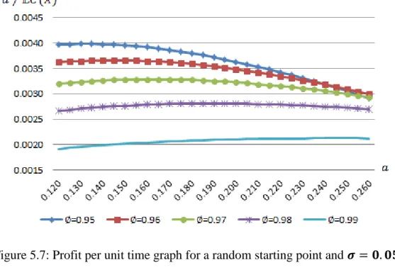
Table 5.14: Optimal trade-in points for ∅ values between 0.95 and 0.99 for a random starting point process………...39
Table 6.1: Optimal trade-in points for ∅ values between 0.95 and 0.99 for simulated data……….……….……….43
Table 6.2: Estimated parameter values for ∅=0.95….………..48
Table B.1: Model outputs for the pair Fortis-Akbank….………..…...68
Table B.2: Model outputs for the pair Fortis-Şekerbank………...69
Table B.3: Model outputs for the pair Vakıfbank-Şekerbank………...69
Table B.4: Model outputs for the pair Akbank-Vakıfbank………...70
Table B.5: Model outputs for the pair Akbank-Şekerbank………...….70
Table B.6: Model outputs for the pair Fortis-Vakıfbank………...71
Table F.1: Profit per unit time values for 20 samples for ∅=0.95 series...92
Table F.2: Profit per unit time values for 20 samples for ∅=0.96 series...93
Table F.3: Profit per unit time values for 20 samples for ∅=0.97 series...94
Table F.4: Profit per unit time values for 20 samples for ∅=0.98 series...95
Table F.5: Profit per unit time values for 20 samples for ∅=0.99 series...96
Table G.1: Estimated parameter values of simulated data for ∅=0.96...…...98
Table G.2: Estimated parameter values of simulated data for ∅=0.97...…...…...99
Table G.3: Estimated parameter values of simulated data for ∅=0.98...…...….100
xi
Table H.1: Profit per unit time values of 20 samples for ∅=0.95, a2=0.28 and
a2=0.54………...103
Table H.2: Profit per unit time values of 20 samples for ∅=0.96, a1=0.60 and
a2=0.58………...104
Table H.3: Profit per unit time values of 20 samples for ∅=0.97, a1=0.65 and
a2=0.66………...105
Table H.4: Profit per unit time values of 20 samples for ∅=0.98, a1=0.67 and
a2=0.76……….…..…106
Table H.5: Profit per unit time values of 20 samples for ∅ = 0.99, 𝑎1 = 0.99
xii
List of Figures
Figure 4.1: Illustration of trading process……….15 Figure 5.1: Time series graph of Fortis and Akbank stock prices……….21 Figure 5.2: Time series graph of Yapı Kredi Bank and Vakifbank stock prices…...22 Figure 5.3: Time series graph of Yapı Kredi Bank and Garanti Bank stock prices..30 Figure 5.4: Profit per unit time graph for X0 = 0 and σ = 0.05…………..……….34 Figure 5.5: Density graph for ∅ = 0.95, a = 0.135 and σ = 0.05………...37 Figure 5.6: Q-Q plot for ∅ = 0.95, a = 0.135 and σ = 0.05 ………...37 Figure 5.7: Profit per unit time graph for a random starting point and σ = 0.05...40 Figure 6.1: Profit per unit time graph using simulated data………….….………....44 Figure 6.2: The timeline for the investor’s process……….………….……….46 Figure A.1: Time series graphs of Fortis and Akbank ………...………….……….60 Figure A.2: Time series graphs of Fortis and Şekerbank……....………….……...61 Figure A.3: Time series graphs of Vakıfbank and Şekerbank....……….….……….61
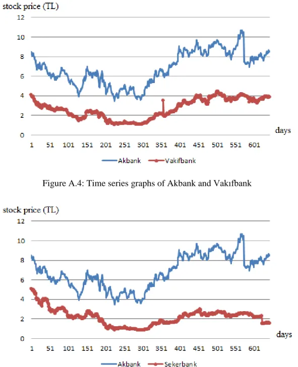
Figure A.4: Time series graphs of Akbank and Vakıfbank…....…………..……….62
xiii
Figure A.6: Time series graphs of Fortis and Vakıfbank……...……….….…...…..63
Figure A.7: Time series graphs of Fortis and Garanti Bank…...……….….……....63
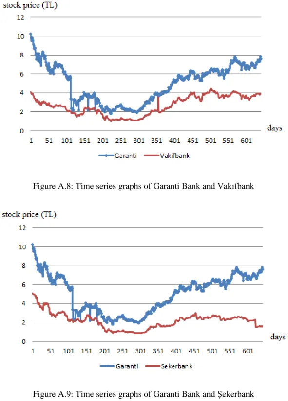
Figure A.8: Time series graphs of Garanti Bank and Vakıfbank ……...….……….64
Figure A.9: Time series graphs of Garanti Bank and Şekerbank…...….…………..64
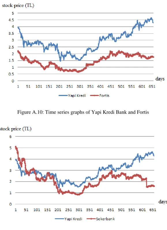
Figure A.10: Time series graphs of Yapı Kredi Bank and Fortis….…...….………65
Figure A.11: Time series graphs of Yapı Kredi Bank and Şekerbank...….………..65
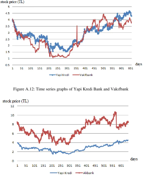
Figure A.12: Time series graphs of Yapı Kredi Bank and Vakıfbank ……...….….66
Figure A.13: Time series graphs of Yapı Kredi Bank and Akbank...….…………..66
Figure A.14: Time series graphs of Yapı Kredi Bank and Garanti Bank…...…....67
Figure A.15: Time series graphs of Akbank and Garanti Bank…...….…………..67
Figure C.1: Profit per unit time for ∅ in [0.95, 0.98], σ = 0.1 and ∆b = 0.005….72 Figure C.2: Profit per unit time for ∅ = 0.99, σ = 0.1 and ∆b = 0.01…………...73
Figure C.3: Profit per unit time for ∅ in [0.95, 0.98], σ = 0.2 and ∆b = 0.01……73
Figure C.4: Profit per unit time for ∅ = 0.99, σ = 0.2 and ∆b = 0.02…....……....74
Figure D.1: Density graph for ∅ = 0.95, a = 0.135 and s = 0.05…...………...76
Figure D.2: Empirical CDF graph for ∅ = 0.95, a = 0.135 and s = 0.05…...77
Figure D.3: Q-Q plot for ∅ = 0.95, a = 0.135 and s = 0.05…...……...77
Figure D.4: Density graph for ∅ = 0.99, a = 0.245 and s = 0.05…...……...78
Figure D.5: Empirical CDF graph for ∅ = 0.99, a = 0.245 and s = 0.05…...79
Figure D.6: Q-Q plot for ∅ = 0.99, a = 0.245 and s = 0.05…...……...79
xiv
Figure D.8: Empirical CDF graph for ∅ = 0.95, a = 0.275 and s = 0.1…...81
Figure D.9: Q-Q plot for ∅ = 0.95, a = 0.275 and s = 0.1…...……...81
Figure D.10: Density graph for ∅ = 0.99, a = 0.49 and s = 0.1…...……...82
Figure D.11: Empirical CDF graph for ∅ = 0.99, a = 0.49 and s = 0.1…...83
Figure D.12: Q-Q plot for ∅ = 0.99, a = 0.49 and s = 0.1…...……...83
Figure D.13: Density graph for ∅ = 0.95, a = 0.55 and s = 0.2…...……...84
Figure D.14: Empirical CDF graph for ∅ = 0.95, a = 0.55 and s = 0.2…...85
Figure D.15: Q-Q plot for ∅ = 0.95, a = 0.55 and s = 0.2…...……...85
Figure D.16: Density graph for ∅ = 0.99, a = 0.98 and s = 0.2…...……...86
Figure D.17: Empirical CDF graph for ∅ = 0.99, a = 0.98 and s = 0.2…...87
Figure D.18: Q-Q plot for ∅ = 0.99, a = 0.98 and s = 0.2…...……...87
Figure E.1: Expected profit per unit time for ∅ in [0.95,0.98], σ = 0.1 and ∆b = 0.005...88
Figure E.2: Expected profit per unit time for ∅ = 0.99, σ = 0.1 and ∆b = 0.01..89
Figure E.3: Expected profit per unit time for ∅ in [0.95,0.98], σ = 0.2 and ∆b = 0.01...89
Figure E.4: Expected profit per unit time for ∅ = 0.99, σ = 0.2 and ∆b = 0.02...90
1
Chapter 1
Introduction
Pairs trading is a statistical arbitrage strategy with a long history. In the 1980s, Nunzio Tartaglia and his colleagues, a group of scientists from mathematicians, physicists and computer scientists who did not have a solid financial background, worked on Wall Street data to reveal the potential arbitrage opportunities in the equities markets. They used sophisticated statistical methods to develop technical trading programs to search for the arbitrage opportunities and to execute trades automatically, which made them the pioneers in this field. Meanwhile, their programs identified pairs of securities, mostly substitutes of each other, whose prices tended to move together. They traded those pairs with a great success in 1987 and made a $50 million profit. After their great success, this trading method, called pairs trading, has become very popular (Gatev et al. [12]).
Pairs trading is a speculative investment strategy which stems from mispricing one of two related stocks. It offers modest but persistent profits (Peskin and Bourdreau [25]; Gatev et al. [12]). This is a market-neutral strategy which depends on relative pricing of stocks. The strategy is based on identifying pairs of shares whose prices are driven by the same economic forces, i.e. two shares whose prices tend to move together, and then trading them when any temporary deviations occur from their long-run average
2
relationship. The intuition behind this method is that the deviation will be reversed eventually and they will return to their equilibrium relationship since the stocks’ prices tend to move together (Gillespie and Ulph [13]). The deviation in the prices is often because one asset is overvalued to the other asset. When we notice a deviation, we invest in a two-asset portfolio, which we call a pairs trading. We sell the overvalued asset (take short position) and buy the undervalued asset (take long position) (Puspaningrum [26]). When the market returns to the equilibrium, in other words when the deviation of the stock prices from their equilibrium values is revealed, we take opposite positions for both assets and obtain profit from the trade. Although this strategy generally does not create big profits, it creates a hedge against the market so that you can gain profit with a low risk.
In order to be successful in pairs trading, it is crucial to be the first to observe the opportunity. Otherwise, the opportunity is exploited by others, and the spread between pair prices becomes tighter and the potential profit becomes smaller. Another important issue in pairs trading is to decide on the appropriate prices, or deviation, to buy and sell the shares.
Selecting correct pairs is crucial; however, since it is possible to detect related pairs with simple statistical techniques, this also becomes an advantage of pairs trading. Correlation analysis, regression analysis, cointegration or some non-parametric rules can be used to choose the related pairs of stocks. In this study, we identify the stock pairs using cointegration because it is based on mean reversion, which guarantees that the spread between the stocks is temporary and will be closed in the end. In other words, mean reversion assures that although anomalies arise among stock prices in the short-term, they will be corrected in the long-term (Ehrman [8]). Cointegration can be defined as in Definition 1.1.
3
Definition 1.1. Let 𝑋𝑡 and 𝑌𝑡 be two integrated time series. If any linear combination of those series becomes a time series having a lower order of integration, then 𝑋𝑡 and 𝑌𝑡 are called cointegrated.
Definition 1.2. The time series 𝑋𝑡 is integrated of order 𝑑, which is represented as
𝑋𝑡~𝐼(𝑑), if (1 − 𝐿)𝑑𝑋
𝑡 is a stationary process, where 𝐿 is the lag operator.
Many analysts rely on correlation, in order to select the pairs and seek a positively correlated pair. Often, those pairs appear in the same or related sectors (Lin et al. [18]). However, Banerjee et al (1993) and Vidyamurthy (2004) showed that the cointegration technique is more effective than correlation technique for revealing potential profit in temporary pricing anomalies between two stock prices driven by common underlying factors. Correlation and regression analysis yield imprecise long-run equilibrium relationships between the shares and do not necessarily imply mean-reversion; on the other hand, the pairs formed by cointegration technique assures that the spread between the pairs are temporary or reverting (Gatev et al. [12]) which is why we prefer to use cointegration technique in our study to choose the pairs.
In this study, we follow Lin et al (2006) and Puspaningrum et al (2009). In those papers, cointegration is used for choosing the pairs and the goal is to find the conditions under which a preset minimum profit per trade is reached. However, the studies do not consider how long it takes to obtain this preset level and it is very important to know this duration since human beings cannot live forever. In this thesis we also take time into account and propose a pairs trading method that maximizes the long-run profit per unit time.
The remainder of the thesis is organized as follows:
In Chapter 2, we review the literature on cointegration and pairs trading. We summarize the studies dealing with cointegration in order to illustrate the problems this technique is used in, other than pairs trading. In addition, we give examples of existing pairs trading
4
studies. In Chapter 3, we introduce our problem. Then, we elaborate the concept of cointegration. In Chapter 4, we propose our resolution method. Chapter 5 presents a case study on which we apply our method. We use six banks’ stock price data from BIST (Istanbul Stock Exchange). In Chapter 6, we provide the results of the computational experiments using both simulated and historical data to evaluate our proposed method and discuss the success of this study. In Chapter 7, we summarize our findings and discuss possible future research topics.
5
Chapter 2
Literature Review
The literature on pairs trading problems is not very extensive. In addition, most of the studies are applications of specific case studies. Thus, the specific type of pairs trading we work on, which is pairs trading using cointegration method, is rare in literature. In this chapter, firstly we will mention about cointegration based strategies in literature. We will present the studies using cointegration strategy from the fields other than pairs trading in this section. In the second part, we will mention about some basic studies about pairs trading in literature. We will present both type of studies, the studies using cointegration as a pair selection method and the studies using methods other than cointegration, in this section.
2.1 Cointegration-based Strategies
Walls (1994) studied the linkages between natural gas spot prices at various production fields, pipeline hubs, and city markets in US Natural Gas Industry using cointegration rank test. Natural gas spot market data are used for likelihood based tests for cointegration. In that study, Johansen method is used for spatial market linkages. The results of that study shows that the natural gas spot markets are strongly correlated. 19
6
market pairs are examined and 13 of the pairs satisfied the rules for perfect market integration.
Chan, Benton and Min (1997) compare 18 nations’ stock markets over a 32-year period. Johansen’s cointegration test is used to analyze the cross country market efficiency. They show that a small number of stock markets are cointegrated.
Bala and Mukund (2001) conducted a study based on the linkage between the US and Indian stock markets. In this study, the theory of cointegration is used to show the interdependence level of Bombay stock exchange and BSE & NYSE & NASDAQ. They concluded that the markets are not interdependent during the selected time period.
Long-run equilibrium relationship and short-run dynamic relation between the Indian stock market and the developing countries’ stock markets are studied by Wong, Agarwal and Du (2005). They examine the Granger causality relationship and the pairwise, multiple and fractional cointegrations between the Indian stock market and the other stock markets in US, UK, Japan. They concluded that the Indian market is closely cointegrated with US, UK and Japan stock markets. With a common fractional, nonstationary component Indian stock index and the other stock indices form fractionally cointegrated relationship in the long run. That study also uses the Johansen method to identify the cointegration relationships.
Narayan (2005) studied the saving investment correlation for China over periods 1952-1998 and 1952-1994. The study revealed that saving and investment are correlated for China for the both periods. They applied residual based tests for cointegration between China’s saving and investment for the two periods.
2.2 Pairs Trading and Statistical Arbitrage Studies
In 2003, Nath studied securities in the highly liquid secondary market for U.S. government debt over 1994-2000. While most of the studies in this field use daily data,
7
intraday data are used in this study. Four different opening and closing thresholds are used to discover the patterns of the security market. He concluded that 15th percentile as opening trigger and 5th percentile as closing trigger is profitable for U.S. security market. Hong and Susmel (2003) conducted a study on pairs trading strategies in which they used cointegration as a pair detection strategy. They worked on 64 Asian shares listed in their local markets and listed in U.S. as American Depository Receipts. They found that if an investor waits for one year before closing his trade-in pairs trading, he can obtain an annualized profit of more than 33%. Also, they stated that market frictions, such as different trading hours, make the strategies risky and hard to implement.
Lin et al. (2006) study pairs trading using cointegrated series to reveal pairs. They develop a pairs trading method to satisfy a preset minimum profit per trade. They illustrate the success of their method on both simulated and real data. They use daily closing price data for two Australian Stock Exchange quoted bank shares, ANZ and ADB, over 18 months to test the results. We will elaborate on that paper because we will use it later to take a further step. Two share prices 𝑃1(𝑡) and 𝑃2(𝑡), chosen using cointegration technique, are taken at time 𝑡 and the number of shares in short position and in long position at time 𝑡 are denoted by 𝑁1(𝑡) and 𝑁2(𝑡), respectively. Let 𝑃1(𝑡) + 𝛽 𝑃2(𝑡) = 𝜀𝑡 denote the cointegration equation where 𝜀𝑡~𝐼(0), i.e. 𝜀𝑡 is integrated of order 1, and 𝑡 ≥ 1 for some 𝛽 < 0. Then two points 𝑎 and 𝑏 are chosen such that 𝜀𝑡𝑜 > 𝑎 > 0 and 𝜀𝑡𝑐< 𝑏, where 𝑡𝑜 shows the time of opening a trade and 𝑡𝑐 shows the time of closing a trade, and the integer 𝑛 >(𝑎−𝑏)𝐾|𝛽| is chosen, where 𝐾 is the minimum preset profit per trade. The trading rule is that we open a trade at 𝑡o when 𝑃1(𝑡o) > 𝑃2(𝑡o) and
𝜀𝑡o > 𝑎 > 0, buy 𝑛 shares of 𝑆2 and sell 𝑛
|𝛽|+ 1 shares of 𝑆1 at time 𝑡o. Then, we close
out the trade at time 𝑡𝑐 when 𝜀𝑡𝑐 < 𝑏 which ensures that the gain is at least 𝐾 monetary
8
Do et al. (2006) propose an approach for pairs trading in a continuous time setting. They assume asset prices follow mean reverted process. They present an EM algorithm to estimate model parameters.
Gatev et al. (2006) conduct an empirical study on pairs trading with daily stock data over 1962-2002. They use a minimum distance of two historical standard deviations between normalized historical prices as the trigger of a trade. When the spread between the stock prices becomes more than this pre-specified threshold, they trade-in. When the spread becomes tighter, which is less than the pre-specified threshold, they trade-out. They tested their method in the presence of transaction costs and their study proved robustness to estimates of transaction costs. They find that the profits have a very small correlation with the spreads between small and large stocks, and between value and growth stocks.
Khandani and Lo (2007) study statistical arbitrage on a number of quantitative long/short equity hedge funds. They discuss the performance of the Lo-MacKinlay contrarian strategies in the context of the liquidity crisis of 2007. In that paper, market-neutrality is enforced by ranking stock returns by quantiles and trading “winners-versus-losers”, in a dollar-neutral fashion.
Papadakis et al. (2007) conduct a study on the impact of accounting information events, such as earnings announcements, on the profitability of pairs trading strategy proposed by Gatev et al. (2006). They find that trades are mostly triggered around accounting information events for the portfolio of U.S. stock pairs between years 1981 and 2006. In addition, they find that the trades opening after those events are less profitable than the trades opening during non-event periods.
Avellaneda and Lee (2008) present a systematic approach to statistical arbitrage and for constructing market-neutral portfolio strategies based on mean-reversion. The approach presented in their study is based on decomposing stock returns into systematic
9
components. The paper compares the ETF and the PCA methods by reproducing the results of Khandani and Lo (2007).
Mudchanatongsuk et al. (2008) propose a stochastic control approach for pairs trading strategy. They work on log-relationship between pairs and modeled them as an Ornstein-Uhlenbeck process. They test the method with simulated data.
Engelberg et al. (2009) discuss the concept of liquidity in pairs trading. They found that the profits are higher when the spread between the prices of the pairs is because of news that temporarily reduces the liquidity of one or both of the stocks in the pair. Also, the profits are lower when the spread between the prices is relevant to the news about the value of a stock in the pair.
Puspaningrum et al. (2009) conducted a study on pairs trading which they used cointegration technique to select the pairs for the trade. They use the stationarity properties of errors of the cointegrated pairs which follow AR(1) processes. They explore how the preset boundaries to open a trade affect the minimum total profit over a specified trading horizon. They estimated the number of trades over a specified trading horizon by using the average trade duration and the average inter-trade-interval. They developed numerical algorithm to estimate the average trade duration, the average inter-trade-interval, and the average number of trades and to maximize the minimum total profit.
Do and Faff (2010) discuss the performance of pairs trading over years. They reveal that as opposed to the continuing downward trend in profitability of pairs trading over years, that strategy worked well during periods of recent global financial crises.
10
Chapter 3
Problem Definition
In this study, our objective is to find a cointegration based pairs trading strategy maximizing the profit per unit time. We are inspired by the study of Lin et al (2006), which is about developing a pairs trading method to satisfy a minimum profit per trade. Although they ensure gaining a preset profit per trade in this strategy, time horizon to obtain that amount of profit is not considered, which may lead the cycle of a trade to be very long. Thus, we take the topic from this aspect in this study.
3.1 Maximizing Profit per Unit Time in Pairs Trading
We intend to find two cointegrated stock pairs, 𝑃1 and 𝑃2, whose cointegrating error is integrated of order 0, i.e. follows a stationary process as in
𝑃1(𝑡) + 𝛽 𝑃2(𝑡) = 𝑋𝑡, where 𝑋𝑡~𝐼(0). (1) This relationship ensures us that the two stocks follow similar patterns, that is decrease and increase at similar points of time, due to the nature of cointegration, which implies mean-revertion.
11
The cointegration equation identifies our portfolio, which consists of 1 stock of 𝑃1 and 𝛽 stocks of 𝑃2. We intend to build a method for pairs trading such that a preset price level for our portfolio initiates each trade. That is, before we start to trade, we set a point 𝑎 such that whenever 𝑋𝑡 exceeds point 𝑎 we trade-in. 𝑎 can be point that the spread between 𝑃1 and 𝑃2 are wide enough to earn from the trade. We short sell the outperforming stock and buy the underperforming stock at this point; in other words, we trade-in. To trade-out, we wait for 𝑋𝑡 to reach below point 0, i.e. 𝑋𝑡 ≤ 0, and we take opposite positions for 𝑃1 and 𝑃2 at this point and close the trade.
Although any point that the spread between the prices of 𝑃1 and 𝑃2 are sufficiently wide works for pairs trading, in order to do a profitable trade, we intend to find the point 𝑎 earning the most. Finding optimal 𝑎, namely the most profitable point is the objective of our study.
Let us show the calculation of profit from this strategy. If we trade-in at point 𝑎 and trade-out at point 0, we gain a profit of 𝑎 from one trading cycle, which makes the profit per unit time equal 𝑎/𝐶 where 𝐶 represents cycle length of one trade of the series 𝑋𝑡. However, note that the first time 𝑋𝑡 reaches to point 𝑎 may realize at a point bigger than point 𝑎. In addition, the first time 𝑋𝑡 reaches to point 0 may also realize at a point smaller than point 0. Thus, the profit per unit time for one trading cycle is at least as large as 𝑎/𝐶. Our goal in this study is to maximize the expected profit per unit time. We benefit from the properties of renewal reward processes to estimate the expected profit per unit time as in (2).
lim 𝑡→∞ 1 𝑡 𝐸 [𝑎 𝐶(𝑡)]⁄ = 𝑎 𝐸[𝐶(𝑡)] (2)
Although the process of stock pricing is continuous, because we use daily stock prices, we can use discrete state space and simplify the problem, which is an advantage for us since we will use Markov Chains to develop the method.
12 3.2 Cointegration
In this section, we explain a key topic of our study, cointegration, which we use for pairs identification.
Many econometric studies are related to long-term equilibrium relation generated by market forces, which makes forming long-term equilibriums an important goal for econometricians. Before the papers published by Granger and Newbold (1974), and Nelson and Plosser (1982), econometricians tended to remove trends and drifts from the models in order to make the variables stationary since most of the techniques in econometrics are based on stationarity. However, with those papers it is indicated that removing trends from the model does not necessarily provide constant unconditional mean and variance over time, which describe stationary series. (Dolado, Gonzalo and Marmol, [7]).
Cointegration is the field of study to seek a linear combination of nonstationary variables which forms a stationary process. In 1981, Granger introduced the notion of cointegration and in 1987, Engle and Granger elaborated it. Then, Johansen introduced the Johansen Test, which allows for more than one cointegration relationship between 2 time series.
Before elaborating the concept let us begin with the definitions of integration and stationarity.
Definition 3.1. A series whose mean, variance and autocorrelation are constant over time
is called stationary.
Definition 3.2. A series with no deterministic component which has a stationary,
invertible, ARMA representation after differencing d times, is said to be integrated of order d. (Engle and Granger [11])
13
Let us consider a vector of economic variables 𝑥𝑡 and let 𝛽be the vector of coefficients of those variables. Then, the system is in equilibrium if 𝛽𝑥𝑡 = 0. If this system does not equal zero, but if there is an equilibrium error 𝜀𝑡 such that 𝛽𝑥𝑡= 𝜀𝑡, then the series 𝜀𝑡 must be stationary for the equilibrium to be meaningful (Enders [8]).
Let us restate the concept according to Engle and Granger’s definition:
Definition 3.3. The components of the vector 𝑥𝑡= (𝑥1𝑡, 𝑥2𝑡, . . , 𝑥𝑛𝑡)′ are said to be
cointegrated of order 𝑑 ≥ 0, 𝑏 > 0, denoted by 𝑥𝑡~ 𝐶𝐼(𝑑, 𝑏) if
i. All components of 𝑥𝑡 are integrated of order 𝑑.
ii. There exists a vector 𝛽 = (𝛽1, 𝛽2, .. , 𝛽𝑛) such that the linear combination 𝛽𝑥𝑡 = 𝛽1𝑥1𝑡+ 𝛽2𝑥2𝑡+ . . + 𝛽𝑛𝑥𝑛𝑡 is integrated of order (𝑑 − 𝑏).
The 𝛽vector is called the cointegrating vector.
As Definition 3.3 states, cointegration does not necessarily remove integration. It is a method to decrease the level of integration. However, in this study we need our portfolio to be a stationary series, thus; we require the pairs be cointegrated of order (𝑑, 𝑏) where 𝑑 = 𝑏.
Note that there may be more than one cointegrating vector to decrease the level of integration of 𝑥𝑡. In fact, if there are 𝑛 components of 𝑥𝑡, then the maximum number of cointegrating vectors is 𝑛 − 1. Because we work with pairs, the vector 𝑥𝑡 has two components, which leads only one cointegrating vector for each pair of stock price series.
Although cointegration can also be formed among more than 2 variables, in this study we use cointegration between 2 variables, because we work with two stock portfolios.
14
Chapter 4
Proposed Pairs Trading Method
Before starting to develop our method let us remind that our objective is to maximize long-run expected profit per unit time in trading process. Firstly, let us give a representation of the series we will analyze. Since we work on stationary linear combinations of nonstationary pairs, we ignore the pairs now on and continue with the whole portfolio, i.e. the series 𝑋𝑡 which is represented as (1). Because the stock prices fit
to autoregressive processes in many studies in literature, we assume that 𝑋𝑡 follows an autoregressive process without intercept of order 1, i.e. 𝐴𝑅(1), as in
𝑋𝑡 = ∅𝑋𝑡−1+ 𝜀𝑡, (3)
where −1 < ∅ < 1 and 𝜀𝑡~𝐺𝑠𝑛(0, 𝜎𝜀2). Note that an 𝐴𝑅(1) process is stationary as long
as its regression coefficient ∅ takes a value strictly between −1 and 1. We assume this holds for now, but we will examine if this assumption holds for our empirical work in the next chapter. Let us remind that means and variances of stationary processes do not change over time which is why we prefer to use in pairs trading. This property of stationarity ensures us that our portfolio returns to mean eventually. In other words, we are confident that our process tend to return its mean 0, i.e. the trade-out point, which is the point to close the trade in our strategy.
15
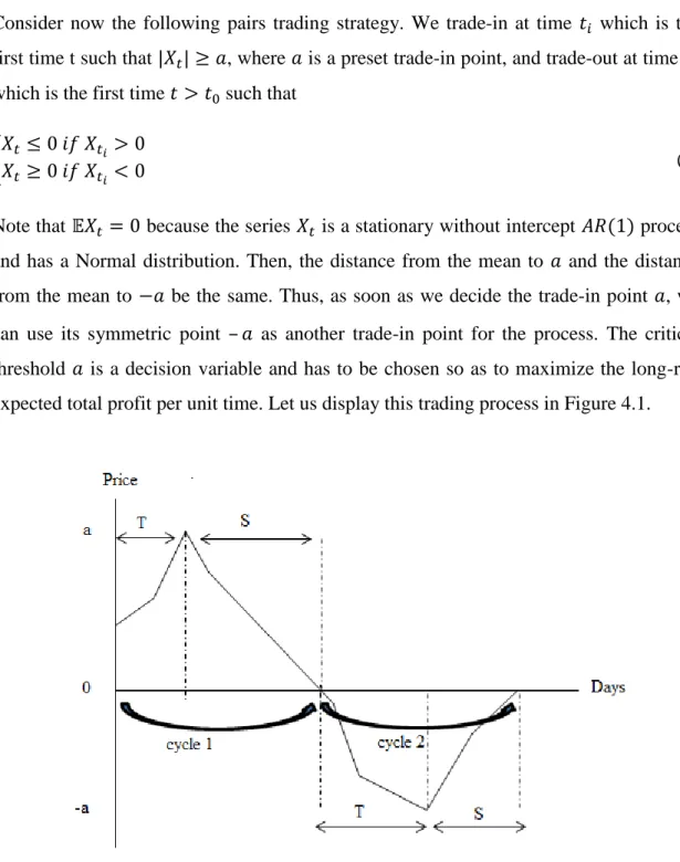
Consider now the following pairs trading strategy. We trade-in at time 𝑡𝑖 which is the first time t such that |𝑋𝑡| ≥ 𝑎, where 𝑎 is a preset trade-in point, and trade-out at time 𝑡0 which is the first time 𝑡 > 𝑡0 such that
{𝑋𝑡 ≤ 0 𝑖𝑓 𝑋𝑡𝑖 > 0
𝑋𝑡 ≥ 0 𝑖𝑓 𝑋𝑡𝑖 < 0 (4)
Note that 𝔼𝑋𝑡 = 0 because the series 𝑋𝑡 is a stationary without intercept 𝐴𝑅(1) process and has a Normal distribution. Then, the distance from the mean to 𝑎 and the distance from the mean to −𝑎 be the same. Thus, as soon as we decide the trade-in point 𝑎, we can use its symmetric point – 𝑎 as another trade-in point for the process. The critical threshold 𝑎 is a decision variable and has to be chosen so as to maximize the long-run expected total profit per unit time. Let us display this trading process in Figure 4.1.
16
Let 𝑇 be the duration up to we trade-in and 𝑆 be the duration between the points we trade-in and trade-out. Then we can define the expected cycle length of a trade as
𝔼𝐶(𝑥) = 𝔼𝑥[𝑇 + 𝔼𝑋𝑇𝑆] (5)
where 𝑋0 = 𝑥, −𝑎 < 𝑥 < 𝑎 and 𝔼𝑥 is the conditional expectation given 𝑋0 = 𝑥. Then, 𝑎 ⁄ 𝔼𝐶(𝑥) becomes the long-run expected reward per unit time by renewal reward theorem. Notice the trade off in the choice of point 𝑎; as 𝑎 increases maximum profit increases; however, 𝑇 and 𝐶(𝑥) also increase. Thus, the relationship between 𝑎 and the profit per unit time is not trivial.
To simplify the problem, we discretize both time and state space of 𝑋 and assume that 𝑋 is a Markov Chain. Let us tackle this problem in two parts. Firstly, let us consider the trade-in process, and then we will consider the trade-out process.
Let 𝛦̂ be the state space for trade-in process as (6).
𝛦̂ = {−a + 1, … , −1, 0, 1, … , a − 1, a, −a} (6) Let 𝑃̂ be the one-step transition probability matrix for the process to trade-in. Note that 𝑎 and −𝑎 be absorbing states for trade-in process. In other words, the trade-in process ends when 𝑋𝑡 touches to points 𝑎 or – 𝑎. Notice that 𝑎 and −𝑎 are not absorbing states for the whole process; however we temporarily makes this assumption in order to calculate the length of trade-in process. We partition the 𝑃̂ matrix as in Table 4.1, so that the 𝑄̂ component of the matrix has the entries 𝑖𝑗 where 𝑖 and 𝑗 are both transient states and the 𝑅̂ component has entries 𝑖𝑗 where 𝑖 is transient but 𝑗 is absorbing. In the matrix, 0̂ shows the zero matrix and 𝐼̂ shows the identity matrix.
17
Table 4.1: Probability matrix representation for process of the strategy
Then the probability of 𝑋𝑡 being at point 𝑎 at time 𝑇, starting from point 𝑥, becomes
𝔈̂(𝑥, 𝑎): = 𝑃(𝑋𝑇 = 𝑎|𝑋0 = 𝑥} = 𝑊̂ 𝑅̂(𝑥,𝑎) (7) where
𝑊̂ = 𝐼̂ + 𝑄̂ + 𝑄̂2+ 𝑄̂3 + ⋯ = (𝐼̂ − 𝑄̂)−1 (8)
as shown for example by Karlin and Taylor [16].
Now let us remove the assumption that 𝑎 and −𝑎 are absorbing states and define our real state space as in (9).
𝐸 = {−b, −b + 1, … , −a, −a + 1, … , −1, 0, 1, … , a, a + 1, … , b − 1, b} (9) where 𝑏 is defined by
𝑏 = 5𝜎 (1 − ∅)⁄ (10)
We use 𝑏 value as an approximate limit for the points 𝑋𝑡 can take at most. The value of 𝑏 ensures that the probability that 𝑋 go outside [−𝑏, 𝑏] is negligible, because,
𝑋1|𝑋0 = 𝑥~𝐺𝑠𝑛(∅𝑥, 𝜎2) (11)
We discretize [−𝑏, 𝑏] in a regular grid with step size ∆𝑏. Then, the state 𝐸 has a total of 2𝑏
∆𝑏
18 𝑃𝑖𝑗 = 𝑃 {(−𝑏 + (𝑗 − 1)∆𝑏 − 𝑏 + 𝑗∆𝑏) 2 < 𝑋1 < (−𝑏 + 𝑗∆𝑏 − 𝑏 + (𝑗 + 1)∆𝑏) 2 | 𝑋0 = −𝑏 + 𝑖∆𝑏} = ∫(−b+jΔb−b+(j+1)Δb)/2σ√2π1 . exp{−(y − ∅(−b + i Δb))2 / (2𝜎2)} (−b+(j−1)Δb−b+jΔb)/2 dy = Φ( (−b+(j+1) Δb−b+jΔb) 2 −ϕ(−b+iΔb) σ ) – Φ( (−b+(j−1)Δb−b+jΔb) 2 −∅(−b+iΔb) σ ) (12)
where −𝑏 ≤ 𝑗 ≤ 𝑏. Note that σ represents the standard error of regression of the process and the mean of the process becomes ∅(−𝑏 + 𝑖∆𝑏) where ∅ is the coefficient of the 𝐴𝑅(1) process. If 𝑗 = −𝑏, 𝑃𝑖𝑗 = 𝑃{𝑋1 <(−𝑏−𝑏+1)2 |𝑋0 = −𝑏 + 𝑖∆𝑏} = Φ( (−b−b+1) 2 −∅(−𝑏+𝑖∆𝑏) 𝜎 ) (13) If 𝑗 = 𝑏, 𝑃𝑖𝑗 = 𝑃{(𝑏+𝑏−1)2 < 𝑋1|𝑋0 = −𝑏 + 𝑖𝑏} = = 1 − Φ( (b+b−1) 2 −∅(−𝑏+𝑖∆𝑏) 𝜎 ) (14)
The expected cycle time of one trade is represented as shown in (2), where 𝑇 is the time it takes until the process trades in and 𝑆 shows the time it takes until the process trades out. Then,
19
Let us define 𝑉(𝑥) and 𝑈(𝑥) as (15) and (16) in order to restate 𝔼𝐶(𝑥) in a closed form.
𝑉(𝑥) = 𝔼𝑥𝑇 (16)
𝑈(𝑥) = 𝔼𝑥𝑆 (17)
So, 𝑉(𝑥) shows the expected time it takes until the process trades in and 𝑈 function shows the expected time it takes until the process trades out when it starts from the trade-in point 𝑥 at time 𝑇. Then, the expected cycle length of one trade becomes 𝑉(𝑥) + 𝔼𝑥[𝑈(𝑋)]. Then,
𝔼𝐶(𝑥) = 𝑉(𝑥) + Σ−𝑏≤𝑦≤−𝑎 𝑜𝑟 𝑎≤𝑦≤𝑏𝑈(𝑦)𝑃{𝑋𝑇 = 𝑦|𝑋0 = 𝑥} (18)
and
𝔼𝐶(𝑥) = 𝑉(𝑥) + Σ−𝑏≤𝑦≤−𝑎 𝑜𝑟 𝑎≤𝑦≤𝑏𝑈(𝑦)𝔈(x, y) (19)
Note that, 𝑉 and 𝑈 functions can also be shown as in (20) and (21) respectively, using the representation in (7). That is, (17) shows the expected number of times the process visits point 𝑗 before being absorbed into ±𝑎, if the process starts from point 𝑖, where −𝑎 < 𝑖 < 𝑎 and −𝑎 < 𝑗 < 𝑎. In addition, (18) shows the number of steps it takes the process to reach to point 𝑗 if it starts from the point 𝑖, where 𝑖 is between the points – 𝑏 and – 𝑎 or between the points 𝑎 and 𝑏.
𝑉(𝑖) = Σ−𝑎<𝑗<𝑎𝑊̂ (𝑖, 𝑗) (20)
and
𝑈(𝑖) = Σ−𝑏≤𝑗≤−𝑎 𝑜𝑟 𝑎≤𝑗≤𝑏𝑊(𝑖, 𝑗) (21)
Note that 𝑊̂ (𝑖, 𝑗) in (20) comes from the calculations of trade-in process while 𝑊(𝑖, 𝑗) in (21) comes from the calculations of trade-out process.
20
Chapter 5
Case Study
5.1 Stock Price Data from BIST
In this study, we work on daily stock prices of six banks in BIST (Istanbul Stock Exchange), Akbank, Şekerbank, Vakıfbank, Garanti Bank, Fortis and Yapı Kredi Bank. We use these stocks for the implementation of the method we develop. We analyze the daily prices of the stocks between years 2008 and 2010.
We check whether there exists cointegration of order (1,1) between the banks’ stock prices we fit to the stationary series, created by the cointegrating linear combinations of the cointegrated pairs and reveal the best-fit time-series models. We also check for the parameters of these time-series models to obtain the most common values those parameters take for the cointegrated stock series we concern. We decide which type of time series model the cointegrated series of Turkish banking stock prices fit the best. Then, we implement our pairs trading method according to that model and the most common estimated parameters. Finally, we measure the performance of our method on the cointegrated pairs of the banking stock prices. We use the statistical package program EViews 5 (Econometric Views) for the analyses of the data.
21
We first check the stocks for stationarity and we found that all stock price series are integrated of order 1. Then, we check for cointegration between the stock prices in order to detect possible pairs. The cointegration tests revealed, 6 cointegrated stock pairs. The cointegration test outputs and the cointegration equations can be found in Tables 5.1 to 5.12 for the pairs. The time series graphs of all the stock pairs are reported in Appendix A. Let us take a look at the patterns of two pairs, one of which has cointegration relationship and the other does not have, in order to illustrate the influence of cointegration on series. Figure 5.1 presents the time series graphs of Fortis and Akbank stock prices. Although there does not exist a perfect match between these two patterns, both stock prices decrease concurrently in the first 300 days, and then start increasing afterwards. The tests show that two stocks are cointegrated.
Figure 5.1: Time series graph of Fortis and Akbank stock prices
As a contrary example, let us inspect two stock prices which are not cointegrated. Figure 5.2 presents time series graphs of Yapi Kredi Bank and Vakıfbank stock prices. Although the stock prices fluctuate similarly, each follows a distinct pattern. For example, around the 350th day Yapi Kredi Bank stock price decreases while Vakıfbank
22
stock price increases abruptly. In addition, around 550th day Vakıfbank stock price suddenly decreases while Yapi Kredi Bank stock price has a continuous increase there. Those signs make a first warning for us for that these two stocks may not be cointegrated. After we conduct cointegration test, the results confirm that Yapi Kredi Bank and Vakıfbank stock prices are not cointegrated. Note that, although the time series graphs often give clear signs for the lack of cointegration between two series, we need to conduct cointegration tests to confirm or reject it.
Figure 5.2: Time series graphs of Yapi Kredi Bank and Vakıfbank stock prices Table 5.1 presents the Johansen Cointegration Test output for the pair Akbank-Fortis. In the first row, Johansen’s Trace Test tests the null hypothesis that the series are not cointegrated, and rejects the null hypothesis with p-value=0.0002. In the second row, the test output for the null hypothesis that there is at most 1 cointegration vector is presented. We cannot reject the null hypothesis since the p-value is 0.7506. The cointegration coefficients are reported in Table 5.2. Thus,
23 is a stationary process.
Table 5.1: Cointegration test output for stocks Akbank and Fortis
Date: 08/28/10 Time: 12:11
Sample (adjusted): 3,642
Included observations: 640 after adjustments
Trend assumption: No deterministic trend (restricted constant)
Series: Akbank – Fortis
Lags interval (in first differences): 1 to 1
Unrestricted Cointegration Rank Test (Trace)
Hypothesized
No. of CE(s) Eigenvalue
Trace Statistic Critical Value Prob. ** None * 0.051549 36.33882 20.26184 0.0002 At most 1 0.003847 2.466900 9.164546 0.7506
Trace test indicates 1 cointegrating egn(s) at the 0.05 level ∗ denotes rejection of the hypothesis at the 0.05 level
∗∗ MacKinnon-Haug-Michelis (1999) p-values
Table 5.2: Normalized cointegrating coefficients for Akbank and Fortis (standard errors in parentheses and c represents intercept coefficient)
Akbank Fortis c
1 -3.734326 -1.499182
(0.23982) (0.36042)
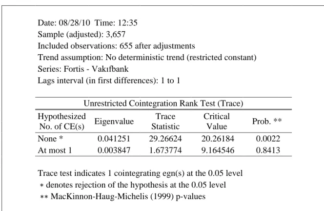
We apply the cointegration test to Fortis-Vakıfbank pair in Table 5.3. The Trace Test rejects that null hypothesis that series are not cointegrated with p-value=0.0022 at ∝= 0.05. On the other hand, the test output for the null hypothesis that there are at most 1
24
cointegration vector cannot be rejected because the p-value is 0.8413. Table 5.4 presents the cointegrating coefficients for that pair. Thus,
𝐹𝑜𝑟𝑡𝑖𝑠 − 0.442035 ∗ Vakıfbank − 0.243589 = 𝑋𝑡 (22)
is a stationary process.
Table 5.3: Cointegration test output for stocks Fortis and Vakıfbank
Date: 08/28/10 Time: 12:35
Sample (adjusted): 3,657
Included observations: 655 after adjustments
Trend assumption: No deterministic trend (restricted constant)
Series: Fortis - Vakıfbank
Lags interval (in first differences): 1 to 1
Unrestricted Cointegration Rank Test (Trace)
Hypothesized
No. of CE(s) Eigenvalue
Trace Statistic Critical Value Prob. ** None * 0.041251 29.26624 20.26184 0.0022 At most 1 0.003847 1.673774 9.164546 0.8413
Trace test indicates 1 cointegrating egn(s) at the 0.05 level ∗ denotes rejection of the hypothesis at the 0.05 level
∗∗ MacKinnon-Haug-Michelis (1999) p-values
Table 5.4: Normalized cointegrating coefficients for Fortis and Vakıfbank (standard errors in parentheses and c represents intercept coefficient)
Fortis Vakıfbank c
1 -0.442035 -0.243589
25
Table 5.5 presents the Johansen’s Test output for Fortis and Şekerbank pair. The Trace Test rejects that null hypothesis that there is at most 0 cointegration equations with p-value=0.0424 at ∝= 0.05. Yet, the test output for the null hypothesis that there are at most 1 cointegration vector cannot be rejected since the p-value is 0.8573. Table 5.6, shows the cointegrating coefficients for Fortis-Şekerbank pair. So, the cointegrating equation becomes
𝐹𝑜𝑟𝑡𝑖𝑠 − 1.308419 ∗ Şekerbank + 1.035947 = 𝑋𝑡, (23) where 𝑋𝑡 is a stationary process.
Table 5.5: Cointegration test output for stocks Fortis and Şekerbank
Date: 08/28/10 Time: 12:45
Sample (adjusted): 3,657
Included observations: 655 after adjustments Trend assumption: No deterministic trend (restricted constant)
Series: Fortis - Şekerbank
Lags interval (in first differences): 1 to 1
Unrestricted Cointegration Rank Test (Trace) Hypothesized
No. of CE(s) Eigenvalue
Trace Statistic Critical Value Prob. ** None * 0.027050 19.54978 20.26184 0.0424 At most 1 0.002422 1.588192 9.164546 0.8573
Trace test indicates 1 cointegrating egn(s) at the 0.05 level ∗ denotes rejection of the hypothesis at the 0.05 level
∗∗ MacKinnon-Haug-Michelis (1999) p-values
26
Table 5.6: Normalized cointegrating coefficients for Fortis and Şekerbank (standard errors in parentheses and c represents intercept coefficient)
Fortis Şekerbank c
1 -1.308419 1.035947
(0.25553) (0.58714)
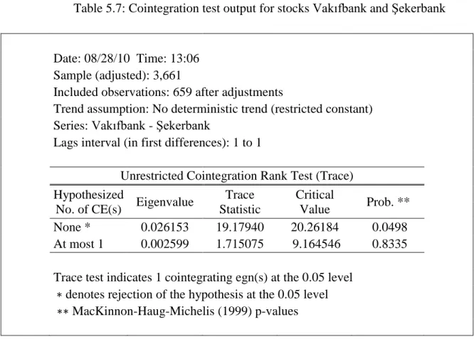
Table 5.7 presents the test output for Vakıfbank-Şekerbank. Johansen’s Trace Test tests the null hypothesis that there are at most 0 cointegration vectors in the first row, and rejects that null hypothesis with p-value=0.0498. However, we cannot reject the null hypothesis that there are at most 1 cointegration vector since the p-value is 0.8335. In Table 5.8, we present the coefficients of that cointegration vector, whose explicit equation is
𝑉𝑎𝑘𝑖𝑓𝑏𝑎𝑛𝑘 − 3.257224 ∗ Şekerbank + 3.375803 = 𝑋𝑡, (24) where 𝑋𝑡 is a stationary process.
27
Table 5.7: Cointegration test output for stocks Vakıfbank and Şekerbank
Date: 08/28/10 Time: 13:06
Sample (adjusted): 3,661
Included observations: 659 after adjustments
Trend assumption: No deterministic trend (restricted constant)
Series: Vakıfbank - Şekerbank
Lags interval (in first differences): 1 to 1
Unrestricted Cointegration Rank Test (Trace)
Hypothesized
No. of CE(s) Eigenvalue
Trace Statistic Critical Value Prob. ** None * 0.026153 19.17940 20.26184 0.0498 At most 1 0.002599 1.715075 9.164546 0.8335
Trace test indicates 1 cointegrating egn(s) at the 0.05 level ∗ denotes rejection of the hypothesis at the 0.05 level
∗∗ MacKinnon-Haug-Michelis (1999) p-values
Table 5.8: Normalized cointegrating coefficients for Vakıfbank and Şekerbank (standard errors in parentheses and c represents intercept coefficient)
Vakıfbank Şekerbank c
1 -3.257224 3.375803
(0.69325) (1.59043)
In Table 5.9, we observe that the Trace Test rejects that null hypothesis that there is at most 0 cointegration equations with p-value=0.0002 at ∝= 0.05 for Akbank and Vakıfbank stock prices. On the other hand, the test output for the null hypothesis that there are at most 1 cointegration vector cannot be rejected because the p-value is 0.7506. Table 5.10 presents the cointegrating coefficients and (25) shows the cointegrating equation for that pair.
28
𝐴𝑘𝑏𝑎𝑛𝑘 − 1.658613 ∗ Vakıfbank − 2.389100 = 𝑋𝑡, (25) where 𝑋𝑡 is a stationary process.
Table 5.9: Cointegration test output for stocks Akbank and Vakıfbank
Date: 08/28/10 Time: 13:38
Sample (adjusted): 3,642
Included observations: 640 after adjustments Trend assumption: No deterministic trend (restricted constant)
Series: Akbank - Vakıfbank
Lags interval (in first differences): 1 to 1
Unrestricted Cointegration Rank Test (Trace) Hypothesized
No. of CE(s) Eigenvalue
Trace Statistic Critical Value Prob. ** None * 0.050353 35.20108 20.26184 0.0002 At most 1 0.003331 2.135571 9.164546 0.7506
Trace test indicates 1 cointegrating egn(s) at the 0.05 level ∗ denotes rejection of the hypothesis at the 0.05 level
∗∗ MacKinnon-Haug-Michelis (1999) p-values
Table 5.10: Normalized cointegrating coefficients for Akbank and Vakıfbank (standard errors in parentheses and c represents intercept coefficient)
Akbank Vakıfbank c
1 -1.658613 -2.389100
(0.09609) (0.27273)
Finally, Table 5.11 presents the Johansen’s Test outputs for Akbank and Şekerbank, in which we observe that the Trace Test rejects that null hypothesis that there is at most 0 cointegration equations with p-value=0.0108 at ∝= 0.05 for Akbank and Şekerbank
29
stock prices. Yet, the test output for the null hypothesis that there are at most 1 cointegration vector cannot be rejected since the p-value is 0.4205. Table 5.12, shows the cointegrating coefficients for Akbank-Şekerbank pair. Additionally, the cointegrating equation is shown in (26).
𝐴𝑘𝑏𝑎𝑛𝑘 − 3.404745 ∗ Şekerbank − 0.416574 = 𝑋𝑡, (26) where 𝑋𝑡 is a stationary process.
Table 5.11: Cointegration test output for stocks Akbank and Şekerbank
Date: 08/28/10 Time: 13:44
Sample (adjusted): 3,642
Included observations: 640 after adjustments
Trend assumption: No deterministic trend (restricted constant)
Series: Akbank - Şekerbank
Lags interval (in first differences): 1 to 1
Unrestricted Cointegration Rank Test (Trace)
Hypothesized
No. of CE(s) Eigenvalue
Trace Statistic Critical Value Prob. ** None * 0.032165 24.86763 20.26184 0.0108 At most 1 0.006143 3.943856 9.164546 0.4205
Trace test indicates 1 cointegrating egn(s) at the 0.05 level ∗ denotes rejection of the hypothesis at the 0.05 level
∗∗ MacKinnon-Haug-Michelis (1999) p-values
30
Table 5.12: Normalized cointegrating coefficients for Akbank and Şekerbank (standard errors in parentheses and c represents intercept coefficient)
Akbank Şekerbank c
1 -3.404745 -0.416574
(0.66968) (1.54808)
Yapi Kredi and Garanti stock prices have no cointegration relationship with any of the banking stock prices. In Figure 5.3, time series graphs of these stocks are presented in the same plot.
Figure 5.3: Time series graphs of Yapi Kredi Bank and Garanti Bank stock prices Revealing the cointegrated stock prices, we can continue with time series model analysis for the stationary series formed by the cointegrated pairs. According to the time series analyses we have conducted, five series turned out to fit to 𝐴𝑅(1) without intercept and
31
one of them, which is the cointegration series of Fortis and Vakıfbank, appears to fit to 𝐴𝑅(2) model. Because most of the pairs fit to 𝐴𝑅(1) model, we pretend that the cointegrated combinations of Turkish banking stock prices follow 𝐴𝑅(1) processes, and we implement our method to Turkish banking stocks case with this assumption. In addition, we estimate the parameters of those 𝐴𝑅(1) models in order to see most common parameter values in the banking sector, which are regression coefficient, i.e. ∅, and the standard error of regression, i.e. 𝜎, for 𝐴𝑅(1) models, so that we can use when we test our method on these data as empirical work in the rest of the study. The estimated parameter values of AR(1) models are reported in Table 5.13. In addition, you can find the model outputs of the stationary series formed from all pairs in Appendix B.
Table 5.13: Parameter estimations of the 𝐴𝑅(1) models
Pair Ø 𝜎 Fortis - Akbank 0.942 0.058 Fortis - Şekerbank 0.985 0.088 Vakıfbank - Şekerbank 0.986 0.236 Akbank - Vakıfbank 0.903 0.245 Akbank - Şekerbank 0.987 0.259
We see that the estimated ∅ values are between 0.903 and 0.987. For our empirical work, we set ∅ values 0.95, 0.96, 0.97, 0.98, 0.99 and examine the results for these parameter values. In addition, the estimated standard error of regression values turn out to be between 0.058 and 0.259 for the cointegrating series of the stock pairs. We set standard error of regression values 0.05, 0.1 and 0.2 for the empirical study.
Although we have stated that those 5 pairs fit to 𝐴𝑅(1) model, they cannot meet the necessary requirements of diagnostic checks for the residuals, such as homoscedasticity or normality of the residuals. Yet, we assume they do and we continue with the assumption that the cointegrated series in concern fit to 𝐴𝑅(1) without intercept model,
32
and we apply our method to 𝐴𝑅(1) models with ∅ between 0.95 and 0.99, and standard error of regression values 0.05, 0.1 and 0.2.
5.2 Profit per Unit Time for 𝑿𝟎 = 𝟎
We have the probabilities to construct the P matrix. Before we obtain optimal trade-in values, i.e. optimal 𝑎 and – 𝑎 points, let us first calculate long-run expected profit per unit time if the process starts from point 0, i.e. 𝑎 ⁄ 𝔼𝐶(0) for the inputs of 𝜎, ∅, ∆𝑏, 𝑏 and 𝑎. The reason we start with the case 𝑋0 = 0 is that 0 is the farthest point to both trade-in points; thus, this case shows the longest time for the process to trade-in. In other words, we start constructing the method for the worst case. However, recall that our aim is to find the optimal, i.e. the most profitable, 𝑎 points for 𝑎 𝔼𝐶(𝑥)⁄ function. Thus, we will extend our study in order to find the most profitable 𝑎 points wherever the process starts at.
We take standard error of regression values, i.e. 𝜎 values as 0.05, 0.1, 0.2, and regression coefficient values, i.e. ∅ values, as 0.95, 0.96, 0.97, 0.98, 0.99. Remember that those 𝜎 and ∅ values are decided from 𝐴𝑅(1) model estimations of the banks’ data in the previous section. We take ∆𝑏 values, which represent the step sizes of the process, at 0.005, 0.01 and 0.02 for our estimations. It is obvious that estimating at different step sizes negatively affects our comparisons. However, we cannot calculate them all at the same ∆𝑏 value since we do the calculations at MATLAB R2007b and as 𝜎 and ∅ values increase MATLAB cannot finish computations in a reasonable time amount unless we also increase step sizes, i.e. ∆𝑏 values.
Let us illustrate the results in Figure 5.4, where σ is taken as 0.05. In the figure, the x-axis shows the trade-in points 𝑎 and the y-x-axis shows the long-run expected profit per unit time values. The step size for 𝜎 = 0.05 is taken as 0.005. Having estimated the optimal objective values, i.e. 𝑎 𝔼𝐶(0)⁄ , for all parameter pairs (∅, 𝜎), we see that the results do not change significantly for different ∅ values at the same 𝜎 value. Thus, even if we fail to estimate the ∅ value correctly for some 𝜎, we still obtain an objective value
33
close to the one for the correct ∅ value. Also note that the objective value as a function of the trade-in value seems to be concave for these 𝜎 values. Moreover, long-run expected profit per unit time decreases as ∅ increases. That is, for ∅ = 0.95 the long-run expected profit per unit time is the biggest and for ∅ = 0.99 the long-run expected profit per unit time is the smallest for the 𝜎 values we concern. The intuition behind this relationship can be explained as
𝑋𝑡− 𝑋𝑡−1= (∅ − 1)𝑋𝑡−1+ 𝜀𝑡 (27)
(∅ − 1) shows the change, or speed, of the 𝐴𝑅(1) process. Since ∅ takes value between −1 and 1, (∅ − 1) takes values between −2 and 0. Then, as ∅ increases, (∅ − 1) approaches to 0. So, the process slows down.
In addition, note that as ∅ increases, optimal 𝑎 value also increases. Optimal trade-in points are as followings: 𝑎∗ = 0.135 for ∅ = 0.95, 𝑎∗ = 0.145 for ∅ = 0.96, 𝑎∗ = 0.165 for ∅ = 0.97, 𝑎∗ = 0.190 for ∅ = 0.98 and 𝑎∗ = 0.245 for ∅ = 0.99,
34
Figure 5.4: Profit per unit time graph for 𝑋0= 0 and 𝜎 = 0.05
The graphs illustrating profit per unit time for different trade-in points are included in Appendix C for 𝜎 values 0.1 and 0.2.
5.3 Profit per Unit Time for a Random Starting Point
Now, let us remove the restriction we consider in the previous section that the starting point of the trading process is 0, and let the process start at any point between −𝑎 and 𝑎. Because we do not know at which point the process starts, we need the distribution of the starting point 𝑋0.
Note that, although we do not have random starting points for the process, we have trade-out points when the process starts at point 0. We will use this information in order to find the distribution of starting points. Let us conduct a simulation such that we check if the trade-out points come from the same distribution wherever the starting point is. The reason we want to check this assumption is that if it is revealed that the trade-out points come from a stationary distribution, then the starting points also come from this stationary distribution since each trade-out point is a starting point for the next trade
35
cycle. We can make this assumption since we work on a nonstop trading strategy. Because the trade goes on forever, if it exists, starting points must come from a stationary “long-run starting point” distribution. The purpose of this section is to check existence and to calculate, if it exists, that stationary distribution.
We conducted simulation at MATLAB for this investigation. Because we do not know the long-run starting point of the process, the first trading cycle starts at 0. So, we start with simulating the case for 𝑋0 = 0 and let the process trade-in and out for 100 times. Then, we record the 100𝑡ℎ trade-out point, and we repeat this for 1000 times. We write
down those 1000 trade-out points.
Secondly, since the trading should continue indefinitely, we take those 1000 trade-out points as possible starting points. Then, we simulate the case when one of those 1000 possible starting points is chosen as 𝑋0 at random, and again let the process trade-in and out until the 100𝑡ℎ trade-out and record that trade-out point. We repeat that process 1000 times and record those trade-out points as trade-out points when the process starts at a random point. Now, we have two samples, the one with 1000 trade-out points for 𝑋0 = 0 and the one with 1000 trade-out points for a random 𝑋0.
As a next step, we want to check if these two samples come from the same distribution for each parameter pair (∅, 𝜎) to find out if the trade-out points of our process has a stationary distribution. We conduct those simulations for the ∅ values 0.95 and 0.99, and for 𝜎 values 0.05, 0.1, 0.2 at their optimal trade-in points based on long-run expected profit per unit time when the process starts at point 0, i.e. 𝑎 𝔼𝐶(0)⁄ , that we have computed before.
We use Two-Sample Kolmogorov-Smirnov Tests (K-S Test) and Q-Q Plots at R and MATLAB in order to check this hypothesis.
The null hypothesis of Kolmogorov-Smirnov Tests is that the samples are drawn from the same distribution. Kolmogorov-Smirnov Tests and Q-Q Plots confirmed our
36
assumption that the two samples of trade-out points come from the same distribution for all parameter estimations. So, the trade-out points have stationary distribution wherever the process starts at. Thus, we can also conclude that the starting points of our process have also stationary distribution.
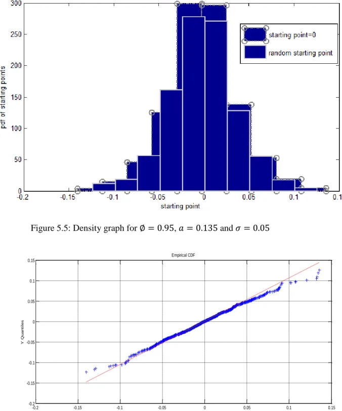
Figures 5.5 and 5.6 present density and Q-Q plots for 𝜎 = 0.05, 𝑎 = 0.135 and ∅ = 0.95. In Appendix D, D statistics and p-values of Two Sample Kolmogorov-Smirnov Test, the probability and cumulative density graphs, and the Q-Q Plots for all (∅, 𝜎) pairs are reported.
As an example, let us examine the density graph and Q-Q Plot for ∅ = 0.95, 𝑎 = 0.135 and 𝜎 = 0.05. Figure 5.5 is the histogram plot for the two series, the series of the trade-out points when the trading process starts from 0, and the series of the trade-trade-out points when the process starts from a random point. According to the graphs, those two series seem fit to the same distribution. Q-Q plot in Figure 5.6 also supports our hypothesis that they come from the same distribution. We see that the Q-Q follows the 45° line y=x, which suggests the identical distributions according to this Probability Plot. The p-value for the Two Sample K-S Test is 0.9689, which fails to reject the null hypothesis of the test that the two samples come from the same continuous distribution. Although, the density functions in Figure 5.5 resemble the Gaussian distribution, the one sample K-S Test reveals that they are different than Gaussian distribution. Because we only need to know that the two samples come from the same distribution, our study is not affected.