Design and implementation of internal MRI coils using ultimate intrinsic

DESIGN AND IMPLEMENTATION OF

INTERNAL MRI COILS USING

ULTIMATE INTRINSIC SNR

A THESIS

SUBMITTED TO THE DEPARTMENT OF ELECTRICAL AND

ELECTRONICS ENGINEERING

AND THE INSTITUTE OF ENGINEERING AND SCIENCE

OF BILKENT UNIVERSITY

IN PARTIAL FULFILLMENT OF THE REQUIREMENTS

FOR THE DEGREE OF

MASTER OF SCIENCE

By

Yiğitcan Eryaman

January, 2007

I certify that I have read this thesis and that in my opinion it is fully adequate, in scope and in quality, as a thesis for the degree of Master of Science.

Prof. Dr. Ergin Atalar (Supervisor)

I certify that I have read this thesis and that in my opinion it is fully adequate, in scope and in quality, as a thesis for the degree of Master of Science.

Prof. Dr. Ayhan Altıntaş

I certify that I have read this thesis and that in my opinion it is fully adequate, in scope and in quality, as a thesis for the degree of Master of Science.

Prof. Dr. Murat Eyüboğlu

Approved for the Institute of Engineering and Sciences:

Prof. Dr. Mehmet B. Baray

ABSTRACT

DESIGN AND IMPLEMENTATION OF INTERNAL

MRI COILS USING ULTIMATE INTRINSIC SNR

Yiğitcan Eryaman

M.S. in Electrical and Electronics Engineering Supervisor: Prof. Dr. Ergin Atalar

January, 2007

In this thesis, methods for optimization of internal magnetic resonance imaging coils have been developed. As a sample optimization endorectal coils were optimized. As the first step ultimate intrinsic signal-to-noise ratio for internal coils was formulated. This value was used as a measure of performance of the internal MRI coils. The related optimization problem was divided into two sub problems: length optimization and cross-sectional optimization. For the length optimization length of a single loop rectangular coil was optimized in order to obtain maximum intrinsic signal to noise ratio at the prostate region. For the cross-sectional optimization designs with different cross-sectional geometries were implemented and tested in saline solution phantom. The designs that gave a significant improvement over the conventional loop coil were favored and the related design ideas were used for the design of an optimized coil. Finally optimized coil was tested in a saline solution phantom model and its performance was calculated.

Keywords: MRI, internal coils, endorectal coil, intrinsic signal to noise ratio,

ÖZET

DAHİLİ MR BOBİNLERİNİN EN İYİ İÇSEL SİNYAL

GÜRÜLTÜ ORANI KULLANILARAK TASARIMI VE

GERÇEKLEŞTİRİMİ

Yiğitcan Eryaman

Elektrik ve Elektronik Mühendisliği Bölümü Yüksek Lisans Tez Yöneticisi: Prof. Dr. Ergin Atalar

Ocak 2007

Bu tezde dahili MR bobinlerinin optimizasyonu için yeni yöntemler geliştirildi. Örnek bir optimizasyon olarak rektum içi bobinler optimize edildi. Başlangıç olarak dahili bobinler için en yüksek içsel sinyal gürültü oranı formüle edildi. Bu oran dahili bobinlerin performansının bir ölçüsü olarak kullanıldı. İlgili optimizasyon problemi uzunluk ve kesit optimizasyonu şeklinde iki alt probleme bölündü. Uzunluk optimizasyonu için dikdörtgen şeklinde bir bobinin uzunluğu prostat civarında maksimum içsel sinyal gürültü oranı verecek şekilde optimize edildi. Bobin Kesidi optimizasyonu içinse farklı kesit geometrisine sahip tasarımlar yapıldı ve bunlar tuz çözeltisi fantomunda denendi. Geleneksel bir diktörtgen bobinden daha iyi çalışan bobinler seçilip bu tasarımların püf noktaları optimize edilmiş yeni bir bobin tasarımı için kullanıldı. Son olarak da optimize edilmiş bobin tuz çözeltisi fantomunda denendi ve performansı hesaplandı.

Anahtar kelimelers: MRG, dahili bobin, rektum içi bobin, içsel sinyal gürültü

ACKNOWLEDGEMENTS

First of all I would like to thank my advisor and my mentor Prof. Ergin Atalar for his academic and psychological support as a supervisor. He was always in his room with his door literally open and ready to help me with all kinds of problems that a graduate student can encounter.

I also want to thank Prof Ayhan Altıntaş for sharing his experience and knowledge with me through my research.

I am also thankful to Prof. Murat Eyüboğlu that he accepted to evaluate my thesis and to be a member of my jury.

Special mention goes to Peter Guion and Dr. İclal Ocak who are from National Institue of Health (NIH). I appreciate the time they spent with me for the MRI experiments and showing me around during my trip to NIH and introducing me to a lot of people working in the field of MRI.

I would also like to mention my friends Haydar Çelik and Onur Ferhanoğlu and thank them for the valuable discussions we made about research, philosophy and certain aspects of life.

Many thanks to Murat and Kemal who are MR technicians at Gazi University for the hours they spent with me in front of the MR console and for sharing their technical experience.

Most importantly I would like thank my family whom I owe everything in life. I would like to thank my older sister Yelda who persuaded my mother and father to have a third child after 14 years. I am grateful to my older brother Yüksel who was there for me as a good friend most of the time. Finally I would like to thank my parents Ahmet and Huriye for being such understanding, friendly and supportive parents.

Table of Contents

1. INTRODUCTION……….. 1

2. EVALUATION OF INTERNAL MRI COILS USING ULTIMATE INTRINSIC SNR………... 7

2.1 Preface………... 7

2.2 Introduction……….. 7

2.3 Theory……… 9

2.3.1 Electromagnetic Field Expression for a Cylindrical Body…... 11

2.3.2 Power Deposited in the Body………... 13

2.3.3 Ultimate Intrinsic SNR for Internal and External Coil Combination………... 14

2.3.4 Ultimate Intrinsic SNR for Solely External Coils………. 15

2.4 SIMULATIONS AND RESULTS………. 18

2.4.1 Optimum Sensitivity Distribution……….. 18

2.4.2 Accuracy Analysis………... 21

2.4.3 Analysis of Loopless Antenna………. 23

2.4.4 Analysis of Endourethral Coil Design………... 28

2.4.5 Parameters for UISNR……… 30

2.5 Discussion………. 33

2.6 Conclusion……… 34

3. GENERAL MANUFACTURING PRINCIPLES OF ENDORECTAL COILS……… 36 3.1 Balun………. 36 3.2 Matching&Tuninng………. 39 3.3 Decoupling……… 42 4. DESIGN OPTIMIZATION………. 46 4.1 Background……….. 46 4.2 Optimization………. 48

4.2.1 Cross Sectional Optimization……….. 48

4.2.1.1 Single Channel Strip Conductor……… 48

4.2.1.2 Dual Phased Array Coil……….. 49

4.2.1.3 Implementation……… 50

4.2.1.4 Intrinsic SNR Calculations………. 50

4.2.1.5 Noise Calculations……… 52

4.2.1.6 Experiments and Results……… 55

4.3 Conclusion………. 62

5. OPTIMIZED ENDORECTAL COIL……… 63

5.1 Design……… 63 5.2 Experiments&Results……….. 65 6. DISCUSSIONS………. 71 7. CONCLUSION………. 76 Appendix A………. 78 Appendix B ……… 85 Appendix C……… 86 BIBLIOGRAPHY……… 87

List of Figures:

Figure 1.1

In situ (cadaver) canine iliofemoral image obtained with an opposed

solenoid catheter probe design.This image was taken from Hurst GC, Hua J, DuerkJL, Cohen AM. Intravascular (catheter) NMR receiver probe: preliminarydesign analysis and application to canine iliofemoral imaging. MagneticResonance in Medicine 1992;24(2):343-357. [5]

Figure 1.2

A rabbit aorta image obtained by a MRI loopless catheter coil. This image was taken from Ocali O, Atalar E. Intravascular magnetic resonance imaging using a loopless catheter antenna. Magnetic Resonance in Medicine 1997;37(1):112-118. [6]

Figure 1.3

Set of prostate images obtained by an endorectal coil during a biopsy sampling session using a MRI compatible manipulator biopsy device. This figure is taken from the publication Krieger et al. Design of a Novel MRI Compatible Manipulator for Image Guided Prostate Interventions Ieee Transactions on Biomedical Engineering, 2005;52(2):306-313 [9]

Figure 2.1:

. a) Cylindrical body model with a coaxial cavity. This model is used for obtaining the UISNR values of an internal and external coil combination. b) A cylindrical body model without a cavity.

Figure 2.2:

Signal reception profile of optimum internal coil (axial H-map). This shows the optimum field pattern inside the body model that will maximize the intrinsic SNR at location

(

ρ=1 mm, =0, z=0φ

)

. A logarithmic intensity scale is employed.

Figure 2.3:

a) Sagittal H-map for the optimum coil. This map is produced on the plane, φ = 0, and the point of interest located at

(

ρ =1 mm, φ =0, z=0

)

is indicated by a star. A logarithmic intensity scale is employed. b) Sensitivity magnitude profile for the optimum coil. H₊ field sensitivity is plotted at x=1 mmin arbitrary units. Both figures show that most of the field energy is concentrated in a narrow region on the z

axis and the greatest brightness indicates where the position of the internal coil should be.

Figure 2.4:

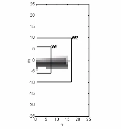
Relative importance of the modes (G-map).This is used for the numerical calculation of the UISNR. The weights of each mode were mapped on the horizontal and vertical axis, representing the m and n modes. The restriction of the modes to those encompassed by bound W2 speeds the calculation with a negligible loss of accuracy (< 1%), whereas use of the overly-restrictive bound W1 results in a 33% error.

Figure 2.5:

A comparison of three ISNR values. ρ₀ is the radial distance of the point of interest from the center of the object. The internal coil is effective at points near the cavity and then the external coil becomes effective as the point of interest approaches the outer boundary on the curve of the UISNR of an internal and external coil combination. In this figure, the external coil has a 20 cm

Figure 2.6:

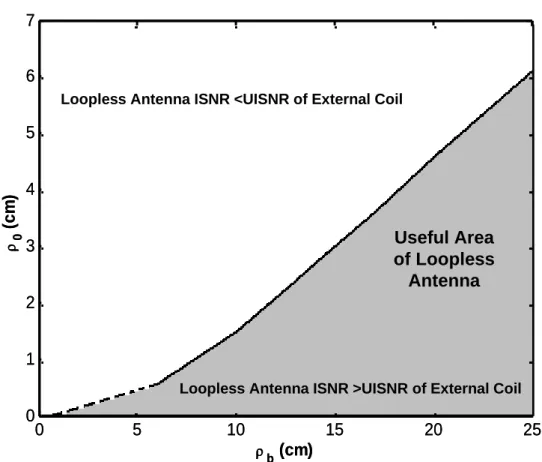
The useful area for the loopless antenna. The SNR values of the loopless antenna and the UISNR of the internal and external coil combination were compared for different values of body radius, ρ_b. For a given body radius, the loopless antenna outperforms the optimum external coil design for points of interest with ρ₀ values that fall in the shaded area. The region at the left bottom of the figure, shown by the dashed line, was found by interpolation.

Figure 2.7:

The performance of the loopless antenna as a function of distance of the point of interest from the center of the object. This figure was obtained by dividing the SNR of the loopless antenna by the UISNR of the internal and external coil combination. In this figure, a 20 cm body radius and a 0.375 mm cavity radius were assumed.

Figure 2.8:

The experimental performance of the endourethral coil design as a function of distance of the point of interest from the center of the object. This figure shows the performance of a single-loop endourethral coil obtained by dividing the experimental SNR value of this coil by the UISNR of the internal coil. UISNR values were computed for a 20 cm radius body with an internal cavity radius of 2.5 mm (cavity size matched the endourethral coil diameter).

Figure 2.9:

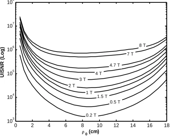
Frequency dependency of the UISNR at various magnetic field strengths. When the point of interest is at a small cylindrical radius, quasi-static conditions are valid and there is then an approximately linear relationship between the UISNR and field strength.

Figure 2.10:

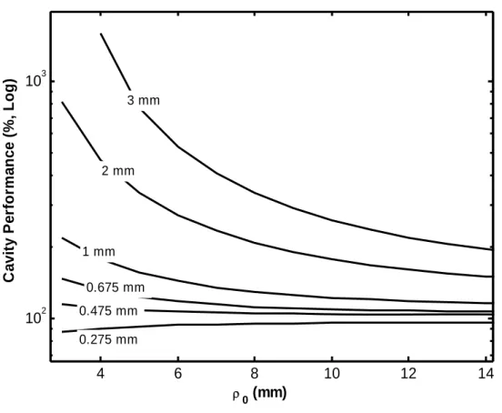
The performance of coils with different cavity sizes. In this figure, different UISNR values for internal coils were compared for different cavity sizes. The comparison was made by dividing the UISNR values of various coils, which have different cavity radii, to the UISNR value of the reference coil, which has a cavity radius equal to 0.375 mm

Figure 3.1

Schematic diagram of a Bazooka balun

Figure 3.2

Figure 3.2 A balun constructed from lumped circuit elements. As it is seen there are two terminals of the balun. Left terminal is connected to the coil and right terminal is connected to the scanner with a coaxial cable.

Figure 3.3

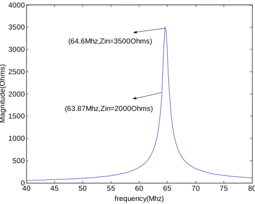
Resonance curve of the balun. Impedance seen on the shunt

capacitor looking at the balun side is plotted.

Figure 3.4

Coil diagram with matching and tuning capacitors

Figure 3.5

Photograph of saline solution phantom. This phantom was used in all experiments.

Figure 3.6

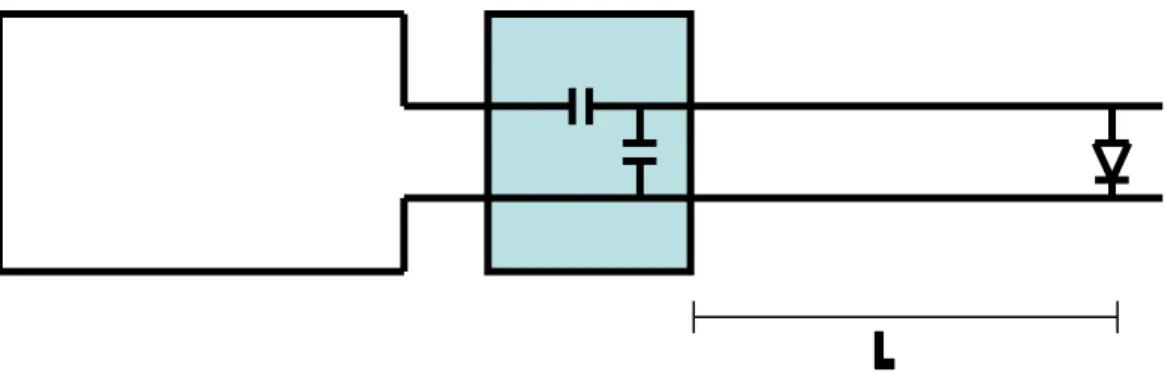
Coil diagram with matching and tuning capacitors and the

decoupling diode Diode is located at a distance L on a two wire transmission line for appropriate decoupling

Figure 3.7

Matching and tuning and the decoupling circuit of the single loop endorectal coil

Figure 3.8

Diode resonance curve: Impedance seen on the shunt capacitor looking to the diode side is observed as a bias voltage of 0,8 V applied on the diode .

Figure 3.9

An endorectal coil ready to be tested for MRI.

Figure 4.1

A prostate image (courtesy of Peter Guion(NIH) )obtained by a endorectal MRI coil. Boarders of the prostate are marked on the image using 4 spots.

Figure 4.2

Endorectal coils with different cross sectional geometries.

Figure 4.3

A noise data sampled from a badly quantized image.

Figure 4.4

A noise data sampled from a well quantized image.

Figure 4.5

A comparison of three endorectal coils ISNR with different cross

Figure 4.6

Improvement ratios due to single channel strip conductor coil and

dual phased array coil. Results are plotted with respect to the radial distance from the coil center.

Figure 4.7

Coil performance ratios plotted with respect to radial distance from

the coil center.

Figure 4.8

Feko v3.2 Simulation model used to simulate single loop

rectangular endorectal coils with different lengths.

Figure 4.9

Coil performance curves for 4 different radial distances are plotted.

Curves are plotted with respect to coil length.

Figure 4.10

Coil performance simulation results of a 4 cm coil, plotted with

respect to radial distance from the coil center.

Figure 5.1

A dual channel coil design that contains a strip-conductor loop.

Figure 5.2

Optimized endorectal coil.

Figure 5.3

S11 of the optimized coil. A minimum reflection coefficient of

0.03 is obtained at 63.87 Mhz

Figure 5.4

S12 parameter of the optimized endorectal coil. S12 is reduced to 0.12 at 63.87 Mhz by decoupling the two channels modifying the width of the copper strip in the design

Figure 5.5

S22 of the optimized coil. A minimum reflection coefficient of

0.13 is obtained at 63.85 Mhz

Figure 5.6

The phantom image obtained by the optimized coil. A fast spin

echo sequence with the following parameters was used. FOV=16cmSlice thickness=3.5mm, Slice interspacing=5mm, bandwidth=41.6 KHz, TR=10000msec, TE=7.75msec.

Figure 5.7

CPM of the optimized coil. Ignoring the artifact on the left side it

can be seen that the coil performed 85% of the maximum attainable SNR Artifact due to the instability of the MRI scanner changes the performance contours by increasing the coil performance in its vicinity

Figure 5.8

Coil performance with respect to radial distance from the coil

center. Performance data is sampled along the vertical axis of the CPM. .

Figure 6.1

Four channel phased array coil design. This design was not

implemented.

Figure A1

Conductivity measurement setup 1. The setup is filled with saline

solution. The coaxial transmission line terminated by an open load at bottom side and the input impedance is measured at the upper end

Figure A2

Conductivity measurement setup 2. The setup is filled with

partially saline solution. The coaxial transmission line is terminated by an open load at bottom and the input impedance is measured at the upper end

Figure A4

The experiment setup for measuring the conductivity. A balun is

List of Tables

Table 4.1

Mean and standart deviation of the distances of the spots X1,X2,X3

and X4 to the coil center

Table 6.1

Rmin values obtained for 3 conductivity values. Variation in R_min is linear with respect to conductivity.

Table A1

Transmission line is filled with saline solution. Input impedance is

measured by the network analyzer using the setup shown in figure 1B Relative permittivity and the conductivity values are also shown

Table A2

Transmission line is half filled with saline solution. Input impedance

is measured by the network analyzer using the setup shown in figure 1B Relative permittivity and the conductivity values are also shown

Table A3

Mean and the standart deviation of the permittivity and the

1. INTRODUCTION

Magnetic Resonance Imaging (MRI) is a medical imaging technology that proved its benefits and became quiet popular among all of the imaging modalities in the past two decades. MRI relies on the fact that the hydrogen atoms (and a few other type of other atoms with odd number of atomic number) found in the human tissues being capable of entering the resonance state under a large main magnetic field. In a MRI scanner patient enters inside the MR bore which generates a very large constant magnetic field. As the spins of the body atoms are in resonance they can be excited using a Radio Frequency pulse generated by RF coils. This excitation disturbs the spins in a way such that when they are returning to their original equilibrium position they emit a weak RF signal with a certain frequency (Larmor frequency). This signal is picked up by a RF receiver coil and then converted into a MR image after certain reconstruction techniques. Goal of many related engineering studies is to optimize this process by concentrating on the different parts of the system.

The receiver coils has an important role in this system since the signal from the body is first picked up by these coils before being converted into regular MR images.

Signal-to-Noise Ratio (SNR) is an important factor in MRI images just as any other imaging modalities. In some situations a high SNR MR image can be the only solution in order to detect a certain tumor or abnormality in a tissue. In MRI there exists a trade off between the SNR, resolution and imaging time. SNR of the MRI images depends on a parameter called Intrinsic Signal-to-Noise Ratio (ISNR) [1]. ISNR can be defined as the SNR per voxel, per square root of time. It is dependant on the coil design and the electromagnetic properties of the body however it is independent of the imaging parameters. Therefore if we design a system that provides high ISNR, we can use this high ISNR for increasing SNR, increasing image resolution or decreasing the imaging time.

As it is mentioned ISNR strongly depends on the coil design. Birdcage coil [2] is an example of RF coil which is most widely used for body and head imaging. There are also phased array receiver coils which are used to image the body extremities [3]. These are some examples of external MRI coils that are clinically used.

An important factor that affects the SNR is the closeness of the receiver coil to the target to be imaged. As the receiver coil gets closer to the target SNR increases. So for imaging targets that are located at the inner region of the human body external MRI coils may not be the best solution. For this purpose internal MRI coils that are placed inside the human body are being used. Internal MRI coils have many application areas in the diagnostic and interventional studies. Their high signal-to-noise ratio properties make them preferable over the external RF coils for many procedures. Various internal MRI coils exist for imaging the inner regions of the human body such as esophagus, urethra, blood vessels and rectum. In 1989 Schnall used an inflatable surface endorectal coil mounted on the inner surface of a balloon structure to obtain high resolution images of the prostate [4]. In 1992 Hurst [5] used a catheter based receiver probe for NMR study of arterial walls. The image below shows the In situ (cadaver) canine iliofemoral image obtained with an opposed solenoid catheter probe design.

Figure 1.1 In situ (cadaver) canine iliofemoral image obtained with an opposed solenoid catheter probe design.This image was taken from Hurst GC, Hua J, Duerk JL, Cohen AM. Intravascular (catheter) NMR receiver probe: preliminary design analysis and application to canine iliofemoral imaging. Magnetic Resonance in Medicine 1992;24(2):343-357. [5]

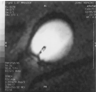
In 1997 Ocali and Atalar presented a loopless catheter coil to be used to image the blood vessels. The device due to its geometrical simplicity could be made in very small dimensions and the electronic circuitry could be kept outside the body without significant loss in imaging performance. A rabbit aorta image is shown in the next figure, obtained by a loopless catheter coil.

Figure 1.2 A rabbit aorta image obtained by a MRI loopless catheter coil. This image was taken from Ocali O, Atalar E. Intravascular magnetic resonance imaging using a loopless catheter antenna. Magnetic Resonance in Medicine 1997;37(1):112-118. [6]

In 1999 a transesophageal coil was introduced by Kendrick A [7]. et al In this study thoracic aorta could be imaged in detail and information about the regional aortic wall motion could be obtained.

Yung [8] used a phased array endorectal MRI coil with a combination of endourethral probe and 3inch surface coil to image a canine prostate. In his study the results he obtained with a phased array combination were compared with the UISNR for external coils. It was shown that such a combination of coils including the endorectal coil outperforms the best external coil within the posterior and the central regions of the prostate 20 times. However his results included comparison to only UISNR for external coils. An optimization with using UISNR for internal MRI coils was not discussed.

Interventional applications which take advantage of the internal MRI coils also exist. Krieger et al in his study used a manipulator biopsy device in order to take biopsy samples from the prostate tissue that is suspected to be a tumor

[9]. An endorectal coil is used as the main imaging device in this system due to its high signal to noise ratio and high resolution advantages. Next set of images shows the prostate obtained by an endorectal MRI coil. Images are obtained during a biopsy process and the clearly show the prostate, biopsy needle and the target on the prostate to be sampled by the needle. The position of the endorectal coil is visible from the high signal profile region inside the rectum in all images.

Figure 1.3 Set of prostate images obtained by an endorectal coil during a biopsy sampling session using a MRI compatible manipulator biopsy device.These images are taken from Krieger et al. Design of a Novel MRI Compatible Manipulator for Image Guided Prostate Interventions IEEE Transactions on Biomedical Engineering, 2005;52(2):306-313 [9]

Although the internal coils have a certain satisfactory performance, by designing coils with higher SNR, better MR images can be obtained to be used for both clinical and interventional purposes. For this reason internal MRI coils should be optimized. In a previous study Ocali and Atalar [10] calculated the ultimate limits of intrinsic SNR for an MRI experiment. After this study as a part of this thesis Ultimate Intinsic Signal-to-Noise Ratio (UISNR) for internal MRI coils were calculated. Other than that, the sensitivity of the optimum coil that generates maximum ISNR at a certain location in the body was

theoretically found. This work was presented first in ISMRM 2004, Toronto [10] Then it was published in Magnetic Resonance in Medicine in 2004 [11]

In this thesis we present a novel method for the optimization of internal MRI coils. UISNR was formulated as a first step of optimization and it was used as a measure of performance for the internal coils. Then endorectal coils are optimized as a sample optimization. Starting with a simple rectangular loop coil we optimized the cross sectional geometry and the length of endorectal coils. Finally an optimized coil is designed, implemented and tested in a water saline solution phantom model. Performance of the coil with respect to UISNR is calculated.

2. EVALUATION OF INTERNAL MRI COILS

USING ULTIMATE INTRINSIC SNR

2.1 Preface

This study was initiated by Imad Amin Abdel-Hafez, who completed an MS thesis on this topic in 2000. Project was restarted in 2003 as two senior projects, by Yiğitcan Eryaman and Haydar Çelik. Project was concluded in 2004 while both of them are in the graduate school. One journal paper and one conference abstact resulted out of this study. While Haydar Çelik became the first author of the journal paper, Yiğitcan Eryaman became the first author of the conference abstract. This chapter was reproduced from the journal publication (Reference: Celik H, Eryaman Y, Altintas A, Hafez IA, Atalar E. "Evaluation of Internal MRI Coils using Ultimate Intrinsic SNR". Magn Reson Med 52:640-649, 2004).

2.2 Introduction

In MRI, the performance of radiofrequency (RF) coils plays a critical role in determining the quality of acquired images. Optimum RF coil designs differ for different imaging locations in the body. Studies about optimum coil designs, however, have generally been performed for a given coil geometry [13,14] There are various types of disposable internal coils, such as opposed solenoids [5,15], expandable coils [16-18], elongated loops [19], and loopless antennas [6], for use in various body cavities, including the vagina, esophagus[7], urethra, blood vessels [20,21], and rectum [22]. Although there is an increase in the SNR of MRI images when these coils are used, it is not possible to make a direct comparison of the performance of internal coils with external coils. Furthermore, there is no formal method by which to evaluate the performance of these internal coil designs in terms of signal-to-noise ratio. Earlier, with a similar motivation, we calculated the ultimate value of the intrinsic SNR

(UISNR) for external coils[10], where the intrinsic signal-to-noise ratio (ISNR) was defined for a given sample-coil combination as the MR signal voltage received from a unit volume of the sample divided by the root-mean-square (RMS) noise voltage received per square-root of bandwidth[1]. Since the ultimate value of the intrinsic SNR is independent of coil design, the information obtained from the UISNR value can be used as a reference to potentially improve the performance of a coil.

In this paper, the calculation of UISNR was reformulated in order to extend it to internal MRI coils [23]. The cylindrical body model is used for both UISNR values, in order to utilize cylindrical symmetry, and coordinates to represent EM fields propagating inside the body. This idea brings simplicity, and does not affect the result negatively. This model has been used by other researchers [24-26], and the results obtained with this model are consistent with previous work. A cylindrical body model with uniform electromagnetic (EM) properties was used to approximate the human body (see Figure 2.1).

Figure 2.1:

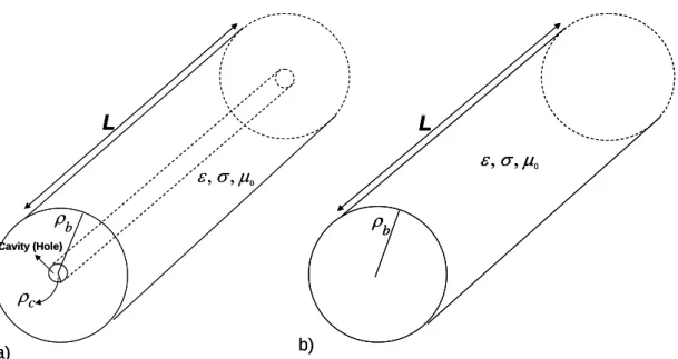
a) Cylindrical body model with a coaxial cavity. This model is used for obtaining the UISNR values of an internal and external coil combination. b) A cylindrical body model without a cavity.

0 , , ε σ μ b ρ L Cavity (Hole) 0 , , ε σ μ c ρ b ρ L a) b) 0 , , ε σ μ b ρ L 0 , , ε σ μ b ρ L L Cavity (Hole) 0 , , ε σ μ c ρ b ρ L L a) b)

In this model, a co-axial cylindrical cavity is assumed to exist at the center of the body, simulating blood vessels or similar structures in which internal RF coils can be placed. With this structure, while surface (or external) RF coils can be placed on the exterior surface of the body, internal coils can be placed in the central cavity.

In order to obtain the signal and noise voltages picked up by a receiving coil, one can use the reciprocity principle and determine the electromagnetic fields generated by the receiving coil when it is used as a transmitter [25]. By assuming that body noise is dominant among other sources of noise, and with the constraint of having a fixed value of the forward polarized component of the magnetic field at the point of interest, SNR can be maximized by minimizing the total power deposited in the body[10]. Therefore, for a given point of interest and electromagnetic (EM) properties of the body, the optimum electromagnetic field distribution must be calculated. As will be shown, this is not only a more general problem than the parametrical optimization of a given coil structure, but also a much easier problem to solve.

The UISNR values for various frequencies and cavity sizes were calculated. The results were used to measure the performance of a loopless antenna [6] and an endourethral coil [20] in the cavity.

2.3 Theory

In the calculation of the ultimate value of the SNR, optimization of the associated electromagnetic field was performed rather than the optimization of a specific coil geometry [10]. UISNR depends on the geometrical and electrical properties of the body and the position of the point-of-interest. We assumed a cylindrical body and the electromagnetic fields inside the human body to be expressed as a weighted sum of the cylindrical waves, which serve as basis functions. To obtain the UISNR value, the noise level in the system should be considered. Power losses, such as conductor losses, radiation losses, and body losses, primarily determine the noise level. For a system with well-designed RF

coils, conductor losses and radiation losses can be minimized and the body loss remains the main factor that limits the SNR value. The expression for the intrinsic signal to noise ratio [13,14], which is independent of imaging parameters, is as shown below,

0 2 4 f b B k R ωΜ Ψ= Τ [1]

where k is the Boltzmann’s constant, _b T is the sample temperature, ω is the

Larmour frequency, and M is the instantaneous magnetic moment per sample ₀

voxel immediately after applying a 900 degree pulse. B is the forward polarized f

magnetic field component and is defined asBf =μHf , where μ is the magnetic

permeability and Hf =

(

Hρ−iHφ

)

/ 2 when the main magnetic field is along the +z direction and for a time convention of j t

eω (suppressed), where i is the

complex number −1. Magnetic permeability in the body is assumed to be uniform and equal to the permeability of free space,μ₀. R is the real part of the input impedance seen by the input terminals of the coil. From the reciprocity principle [25,27], the value of R can be found by calculating the total dissipated power when the receiver coil is used as a transmitter and driven by a 1 amp rms current source from its input terminals.

As mentioned above, the body loss, R_body, is the main factor in power

dissipation and noise level. For a properly designed system R≅R_body and with a

unit rms current excitation, it becomes Rbody =Ploss, where Ploss is power loss in

the body. We assume that outside the body, we have a lossless region; thus, there is no contribution to power dissipation from the fields in the outside region. Since we do not specify the fields outside the body, we do not need to impose boundary conditions.

= ( ( ) + ( )) jm j znz

zmn mn m n mn m n

E A J β ρ_ρ C Y β ρ_ρ e φe− β

zmn = ( mn m( n ) + mn m( n )) jm j znz

H − j B J β ρ_ρ D Y β ρ_ρ e φe− β

In order to obtain maximum SNR, Rbody must be minimized, while H f

must be maximized. Since, with the aid of a simple transformer, the value of

f

H can be modified without affecting the SNR, in our calculations, we

arbitrarily assumed the forward polarized magnetic field at the point of interest,

0

rG , is fixed to 1, i.e., H_f( ) 1r0 =

G

. Therefore, the problem of calculation of the ultimate value of the intrinsic SNR (UISNR) reduces to minimization ofR_body[9].

2.3.1 Electromagnetic Field Expression for a Cylindrical Body

For an infinitely long cylindrical body, the electromagnetic fields can be written in terms of an inverse Fourier transform of cylindrical wave function expansions [26]. When one considers a cylindrical body of finite length, the Fourier integral becomes the Fourier series at discrete spectral values. For the problem considered here, the optimum electromagnetic (EM) field that will minimize power dissipation inside the body can be written as the weighted sum of the cylindrical waves:

mn m n ∞ ∞ =−∞ =−∞ =

∑ ∑

EG EG [2]

where m and n are integer variables representing the Fourier modes (Fourier components).

The cylindrical waves can be generated from the z-components of electric and magnetic field intensities, which are the solutions for scalar Helmholz equations:

[3] [4]

where ε is the electric permittivity, and Jm and Y are mth order first and m

second kinds of Bessel functions, respectively (the second kind of Bessel functions are also called Neumann functions). In addition,

, , C , and

mn mn mn mn

A B D are the unknown weights that need to be determined and

n ρ β is given by 2 2 n zn ρ β = β −β [5] where 2

[

]

0 j j

β =− ωμ σ + ωε . Note that β _{is the wave number in the body and} σ is the conductivity of the body. In general, βzcomprises a continuous

spectrum of cylindrical waves [26]. The field representation above is an alternative to the eigenfunction (modal) representation. They are related through an integration in the complex β_{z plane [28]. Due to the finite length of the} body, βz is limited to a discrete set of real numbers as βzn =

(

2 /π L n

)

, where L

is the length of the body and n is an integer value both positive and negative, corresponding to the Fourier series expansion of the fields. Thus, the EM field becomes periodic along the z direction with a period of L. We will later show that our results do not depend on the value of L, as long as L is large enough.

Using Maxwell’s equations, the other components ( and φ ρ) of the fields in Eq. [13] can be obtained in terms of E_z and H . As an example, consider the _z

two equations below:

z E E j H z φ ρ ρ ωμρ φ ∂ ∂ _{− = −} ∂ ∂ [6] and ( ) z H H j E z ρ φ σ ωε ρ ∂ ₋∂ _{= +} ∂ ∂ [7]

Differentiating Eq. [17]with respect to z and substituting into Eq[18] gives and

E_φ H_ρ components of the field (see Appendix A. For other components,

refer to Maxwell’s equations in [29]. It should be noted that the field expansions are valid for all types of electromagnetic sources. The unknown weights take specific values for a given configuration.

Since j(2 /L nz)

e− π and ejmφ terms are common in all field expressions, for

convenience EG_mn can be expressed as:

(2 / ) j L nz jm mn mn mn EG =E ⋅αG ⋅e φe− π [8] where [ C ]T mn = A_mn B_{mn mn} D_mn αG [9]

and E is a 3-by-4 matrix, and is a function of _mn ρ, but not φ or z . In Eq.[9],

T denotes a transpose operation.

2.3.2 Power Deposited in the Body

The main reason for considering the electromagnetic field as a weighted Fourier sum of cylindrical waves is to find the optimum field, which will minimize the power consumption in the body model. Each cylindrical wave expression serves as a basis function in the expansion of the optimum field. The total power deposited in the body, which is also equal to Rbody, can be calculated

as a volume integral as shown below:

*T body

body

R =σ

∫

E EJG JGdυ [10]

where (*) above the electric field denotes the conjugate operator and dυ is the

differential volume element inside the volume determined by the body model. Note that the conductivity, σ , is taken as uniform throughout the body.

When the field is expressed as the sum of cylindrical waves (see Eq.[2]), the integral becomes:

[11]

where k and l are integers. If the summation is taken out of the integral operator,

body

R can be written as:

[12]

The right-hand side of the above equation is a volume integral and involves integration with respect to ρ φ, , and z variables.

The forward polarized magnetic field, H_f

( )

rG _{can be expressed as:}

( )

mn

( )

mn f mn H rG =

∑

bG r αG G⋅ [13] where bmn

( )

r G K

is a row vector and rG=

(

ρ φ, , z

)

denotes the position of the point of interest in the cylindrical coordinates. The components of bmn

( )

r

G K

are expressed in terms of the components of the magnetic field, as shown in Appendix B.

2.3.3 Ultimate Intrinsic SNR for Internal and External Coil

Combination

In the calculation of UISNR, we assumed a cylindrical object with a co-axial cavity, as shown in Figure 2.1a. It is assumed that there is no electrical loss in the cavity and outside this cylindrical object and all the losses are due to finite conductivity of the object. This structure permitted placement of both internal coils in the cavity and external coils on the surface of the object. Therefore, the following calculation applies to the UISNR for an internal and external coil combination. *T body mn kl mn kl body R =σ ⎛_⎜ ⎞ ⎛_{⎟ ⎜}⋅ ⎞_⎟dυ ⎝

∑

⎠ ⎝

∑

⎠

∫

EG EG *T body mn kl mn kl _body R =

∑∑ ∫

σ EG ⋅EG dυ

* _* 2 body cavity T _T mn mn mn mn mn p L d ρ ρ π σ ⎡⎢ ρ ρ⎤⎥ = ⋅ ⋅ ⋅ ⎢ ⎥ ⎣

∫

⎦ αG E E αG body mn mn R =

∑

p

Because of the cylindrical symmetry of this object, this volume integral in the above equation can be decomposed into three integrals:

[14]

where, ρcavity and ρbody are the hole (cavity) and body radii, respectively (see

Figure 2.1a). Because we only considered the region interior to the body, limits for integration, with respect to the ρ variable, were determined by the cavity and body radii. Note that L is the limit of integration with regard to the z variable. The complexity of the body integral can be reduced by evaluating the integrals with respect to the variables φ and z . With this simplification, the body integral can be written as follows:

[15]

The above equation shows that all modes are orthogonal to each other. This simplification makes it possible to express the R_body as a summation in m and

n only, as below

[16]

where

[17]

The new variable p denotes the power dissipation for each of the modes, and _mn

is also equal to:

[18] 2 / 2 * * ( ) (2 / )( ) 0 / 2 ( ) ( ) body cavity L T T j m k j L n l z mn kl mn kl mn kl body L d d e d e dz ρ _π φ π ρ υ ρ ρ − − φ − − − ⋅ = ⋅ ⋅ ⋅

∫

EG EG

∫

E αG E αG

∫

∫

*T mn mn p =αG ⋅R ⋅αG * _* * 2 , if = and = 0 , elsewhere body cavity T _T mn _{mn kl} kl T mn kl body L d m k n l d ρ ρ π ρ ρ υ ⎧ ⎡ ⎤ ⎫ ⎪ ⋅⎢ ⋅ ⎥⋅ ⎪ ⎪ ⎪ ⋅ _{= ⎨ ⎢⎣ ⎥⎦ ⎬} ⎪ ⎪ ⎪ ⎪ ⎩ ⎭

∫

∫

E E α E E α G G G G

min 1 mn mn R G =

∑

( )

* 1 min mn T opt = _mn− ⋅ mn R αG R bG rG where [19]

It is important to note that Rmn is a Hermitian matrix. This fact simplifies the

calculations, since it requires the computation of the terms only on one side of the diagonal.

The problem of finding the ultimate value of SNR becomes that of finding the optimum αmn

G

values, such that:

* min mn mn T opt _mn opt mn R =

∑

αG ⋅R ⋅αG [20]

with the constraint that Hf( ) 1r0 =

G

. This constrained minimization problem can be solved using standard techniques such as the Lagrange multiplier technique and αoptmn

G

can be found as:

[21] where [22] and

( )

₁ *T

( )

mn mn mn mn G =bG r RG ⋅ − ⋅bG rG [23]

Although m and n values are unbounded, for practical computational

purposes, they need to be limited to a range, and the selection of the proper range will be discussed later.

It is instructive to note that, as L increases, the element values of the R_mn

matrix increase as well; thus, G_mn decreases. On the other hand, the density of

* 2 body cavity T mn L mn mn d ρ ρ π σ ρ ρ ⎡ ⎤ ⎢ ⎥ = ⋅ ⎢ ⎥ ⎣

∫

⎦ R E E

the samples of β_z (note that β_zn =

(

2 /π L n

)

) increases with L. As a result, the

value of R_min becomes independent of L, for sufficiently large values of L.

Once the optimum weights are known for a given point of interest, the forward polarized magnetic field (H ) inside the human body model can also _f

be simulated to show the sensitivity distribution of the optimum coil.

2.3.4 Ultimate Intrinsic SNR for Solely External Coils

In the same cylindrical geometry, if one removes the cavity (see Figure 2.1b), the calculation of UISNR will be solely for external coils since there will be no cavity in which to place an internal coil. In this case, we will need to make some small modifications to the above formulation.

First, ρcavitymust be set to zero. Therefore, the boundaries of the

integrations in Eqs.[15], [17], and [19] should be changed to 0 to ρbody. This

change will render Neumann functions inapplicable, because Neumann functions have singularities at the origin. Therefore, C and mn D must vanish. mn

As a result, in the calculation of the UISNR for external coils, only Bessel J-type functions should be included in the expressions.

Apart from these distinctions, the calculation of UISNR for external coils is identical to the calculation of UISNR for the internal and external coil combination.

2.4 Simulations and Results

A MATLAB (version 6.0,Mathworks Inc., Natick, MA) program was developed to calculate the UISNR values. In all calculations, a uniform conductivity σ of 0.37 Ω-1m-1, a relative electric permittivity ε_r of 77.7, and a relative magnetic permeability μ_rof 1.0 are taken as average values at 64 MHz (or 1.5 T for protons) [10]. The SNR calculations in [30] for the loopless antenna [6] and experimental results for the endourethral coil design [20] were compared with the UISNR values.

2.4.1 Optimum Sensitivity Distribution

The reason for using an internal coil is to obtain better results compared to external coils. For this purpose, sensitivity distribution maps, i.e., the distribution of the forward polarized magnetic field, are used to ensure the dominant effect of the internal coil. In order to demonstrate the distribution, both axial and sagittal views were obtained. We call these distribution maps H-maps. First, a logarithmic intensity scale is employed on the z=0 plane with

respect to φ and ρ (axial H-map). The point of interest was chosen on the

0

z= plane as well. The map was enlarged 100 times to concentrate on a

smaller field of view and to observe the effect of the internal coil. In Figure 2.2, the white cloud around the cavity represents high field magnitudes.

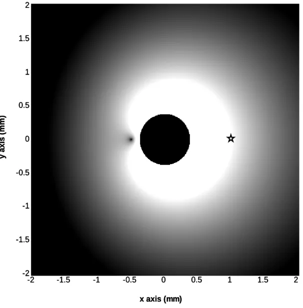
Figure 2.2:

Signal reception profile of optimum internal coil (axial H-map). This shows the optimum field pattern inside the body model that will maximize the intrinsic SNR at location

(

ρ=1 mm, =0, z=0φ

)

. A logarithmic intensity scale is employed.

As is clear from the same figure, the field is concentrated around the cavity (which is shown in black in the middle of the image) but also shifted toward the point of interest. A sagittal H-map is another perspective for a signal reception

-2 -1.5 -1 -0.5 0 0.5 1 1.5 2 -2 -1.5 -1 -0.5 0 0.5 1 1.5 2 x axis (mm) y axi s ( m m ) -2 -1.5 -1 -0.5 0 0.5 1 1.5 2 -2 -1.5 -1 -0.5 0 0.5 1 1.5 2 x axis (mm) y axi s ( m m ) -2 -1.5 -1 -0.5 0 0.5 1 1.5 2 -2 -1.5 -1 -0.5 0 0.5 1 1.5 2 x axis (mm) y axi s ( m m )

profile of the optimum internal coil, obtained on the φ = plane, at the point of 0 interest

(

ρ=1 mm, φ =0, z=0

)

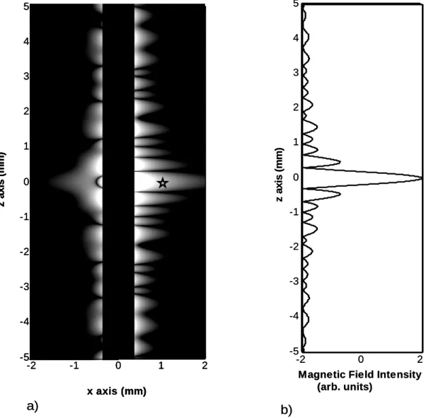
indicated by a star (see Figure 2.3a).

Figure 2.3:

a) Sagittal H-map for the optimum coil. This map is produced on the plane, φ = 0, and the point of interest located at

(

ρ =1 mm, φ =0, z=0

)

is indicated by a star. A logarithmic intensity scale is employed. b) Sensitivity magnitude profile for the optimum coil. H₊ field sensitivity is plotted at x=1 mmin arbitrary units. Both

figures show that most of the field energy is concentrated in a narrow region on the z

axis and the greatest brightness indicates where the position of the internal coil should be. -2 -1 0 1 2 -5 -4 -3 -2 -1 0 1 2 3 4 5 x axis (mm) z axi s ( mm) a) _b) -2 0 2 -5 -4 -3 -2 -1 0 1 2 3 4 5

Magnetic Field Intensity (arb. units) z ax is ( mm) -2 -1 0 1 2 -5 -4 -3 -2 -1 0 1 2 3 4 5 x axis (mm) z axi s ( mm) -2 -1 0 1 2 -5 -4 -3 -2 -1 0 1 2 3 4 5 x axis (mm) z axi s ( mm) a) _b) -2 0 2 -5 -4 -3 -2 -1 0 1 2 3 4 5

Magnetic Field Intensity (arb. units) z ax is ( mm)

Again, a logarithmic intensity scale is employed and enlarged to a smaller field of view. The highest brightness, which shows where the position of the internal coil should be located, occurs approximately between -1 mm and 1 mm on the z direction. Beyond this region, the field is very small with regard to the field at the center, z=0 plane. The point of interest is indicated by a star and is

in the cloud (white region) that represents the field of the internal coil. The appearance of the optimum magnetic field distribution is in line with intuition. In Figure 2.3b, the sensitivity is plotted at x=1 mm. Both figures indicate that

most of the field energy is concentrated in a small region on the z -axis, if we ignore some fluctuations caused, most probably, because of the truncation of the modes.

2.4.2 Accuracy Analysis

In our calculations, some assumptions were used. These assumptions may cause inaccuracy in the results. A detailed analysis of these error sources is necessary.

The length of the body is an important parameter, because, in the formulation, we assumed that the optimum EM field is periodic with the length of the cylinder. Here, we need to verify that this periodicity assumption does not alter the solution significantly. With this purpose, first, body length, L, was taken as 1 m and SNR was calculated for a point of interest

(

ρ =1 cm, φ =0, z=0

)

. Then, the result was compared with the SNR value for an L equal to 2 m and for the same point of interest. Note that in order to keep the range of β_{z constant, the number of n modes was doubled. There was only a} 1% difference between these two results. The same procedure was repeated for different points of interest, and the SNR value did not change more than 1%. Note that at the end of the theory section, it is explained that R_{min is independent}

Although an infinite number of m and n indices are necessary for an exact

result, a restricted number of Fourier modes provides an accurate solution. Thus, in order to check whether there are enough modes, G_mn values are shown in the

form of a map (the m and n are the coordinates of the map), which is useful for showing the importance of each mode used for the numerical calculation of the UISNR. We call this map a G-map (see Figure 2.4). Note that only positive n values are shown because of the symmetry of the problem, i.e., Gmn =Gm₍−n₎

Figure 2.4:

Relative importance of the modes (G-map).This is used for the numerical calculation of the UISNR. The weights of each mode were mapped on the horizontal and vertical axis, representing the m and n modes. The restriction of the modes to those encompassed by bound W2 speeds the calculation with a negligible loss of accuracy (< 1%), whereas use of the overly-restrictive bound W1 results in a 33% error.

The necessary number of modes is decided by investigating the G-map with respect to the variable, n. The number of modes is decided according to the

parameters of the body. For example, the number of modes increases as body length increases. We also observe that as the point of interest gets closer to the boundaries, a greater number of modes in m and n indices are needed.

Although this is the case for most points of interest, the values that determine body resistance, and eventually the UISNR values, are limited to a small range of m and n values; therefore, a finite sum of selected modes is acceptable. In

Figure 2.4, the total number of modes for both m and n is 1250, which is very

high. Including all of these modes is time consuming. If smaller m and n

values are chosen, the window will get smaller, as seen on W1 and W2. For window 1 (W1), the numbers of mand n are insufficient, and the UISNR value

obtained for this window (where m = 6 and n = 7) is 33% less than the UISNR

value of the largest window (m= 50, n= 25). However, W2 (m= 10, n= 17)

provides almost the same UISNR value (a difference of 0.2%) as the largest window; thus, W2 includes the most effective modes and also takes much less time to plot the map. As a result, this mapping method is useful for efficient calculation of the result.

2.4.3 Analysis of Loopless Antenna

The loopless antenna [6] is a very simple antenna design that has been investigated for use in MRI-guided vascular interventions [30]. The design consists of a coaxial cable with an extended inner conductor. Comparing the UISNR values of internal and external coils with the ISNR values of the loopless antenna is important in understanding its performance. The UISNR value of the internal and external coil combination was plotted for a 20 cm-radius body with a 0.375 mm cm-radius cavity as a function of the position of the point of interest in Figure 2.5.

Figure 2.5.

A comparison of three ISNR values. ρ₀ is the radial distance of the point of interest from the center of the object. The internal coil is effective at points near the cavity and then the external coil becomes effective as the point of interest approaches the outer boundary on the curve of the UISNR of an internal and external coil combination. In this figure, the external coil has a 20 cm body radius and the internal and external coil combination has a 20 cm body and a 0.375 mm cavity radii. The radius of the loopless antenna is 0.375 mm.

In the same graph, the intrinsic SNR value of a loopless antenna [29] and the UISNR value that can be obtained from exclusively external coils were

0 2 4 6 8 10 12 14 16 18 20 103 104 105 106 107 ρ₀ (cm) UI S NR ( L o g ) Loopless Antenna UISNR of External Coil

improvement there is in the SNR performance of the loopless antenna. In addition, we can see in what region which coil performs better. For example, at a point of interest

(

ρ =1 mm, φ =0, z=0

)

, the performance of the loopless

antenna is only 4% of the UISNR of an internal and external coil combination. This means that there may be an internal MRI coil design that fits in the same cavity and performs 25 times better than the loopless antenna for that point of interest. It is important to note that the coil design that can result in this significant improvement is not known at this time.

Deciding whether to use the loopless antenna for a specific point of interest is crucial with regard to time saving and therapeutic management. In Figure 2.5, the SNR curve of the loopless antenna and the UISNR of the external coil intersect at one point. This point determines the radius of the “useful region” of an internal MRI coil, the loopless antenna. For points that are closer to the external surface of the body, some external coils, which perform better than the internal coil, may exist. The size of the useful region of an internal coil depends on the body radius. When the body size is large, the useful region of the internal coil increases, whereas, when the body size is small, the internal coil becomes useful for imaging a smaller region. Figure 2.6 shows the radius of the useful area as a function of body size for the loopless antenna. To obtain this plot, the values of UISNR were calculated for external coils and the SNR of the loopless antenna was compared with these UISNR values as a function of body radius.

Figure 2.6:

The useful area for the loopless antenna. The SNR values of the loopless antenna and the UISNR of the internal and external coil combination were compared for different values of body radius, ρ_b. For a given body radius, the loopless antenna outperforms the optimum external coil design for points of interest with ρ₀ values that fall in the shaded area. The region at the left bottom of the figure, shown by the dashed line, was found by interpolation.

For a fixed value of body radius, the SNR values were sampled at 5 mm, and the point where the loopless antenna SNR exceeded the UISNR for external coils was found by interpolation. The same procedure was repeated for different body radius values between 5 cm and 25 cm. Figure 2.6 shows that, at any point of interest in the shaded area of the graph, the SNR of the loopless antenna dominates the UISNR of the external coil and this region is called the useful

0 5 10 15 20 25 0 1 2 3 4 5 6 7 ρ b (cm) ρ 0 (c m )

Loopless Antenna ISNR <UISNR of External Coil

Loopless Antenna ISNR >UISNR of External Coil

Useful Area of Loopless Antenna 0 5 10 15 20 25 0 1 2 3 4 5 6 7 ρ b (cm) ρ 0 (c m )

Loopless Antenna ISNR <UISNR of External Coil

Loopless Antenna ISNR >UISNR of External Coil

Useful Area of Loopless

area of the loopless antenna. As a result, if the point of interest is in the shaded region, the loopless antenna should be used.

Comparing the loopless antenna with the UISNR of an internal and external coil combination allows a determination of how much improvement can be achieved over the loopless design, as well as determining the point of interest where the loopless antenna performs best. The intrinsic SNR values for the loopless antenna were divided by the UISNR of an internal and external coil combination and plotted as a function of the point of interest in Figure 2.7

Figure 2.7:

The performance of the loopless antenna as a function of distance of the point of interest from the center of the object. This figure was obtained by dividing the SNR of the loopless antenna by the UISNR of the internal and external coil combination. In this figure, a 20 cm body radius and a 0.375 mm cavity radius were assumed.

Our sample design loopless antenna achieved maximum performance at the points of interest with a distance to the center of the body around 6.5 cm

0 5 10 15 5 10 15 20 25 ρ₀ (cm) P e rf o rma n c e of Lo opl e s s A n te nn a (%)

(

ρ0 =6.5 cm

)

. For those points, more than 20% of the maximum achievable SNR was obtained (see Figure 2.7).

2.4.4 Analysis of Endourethral Coil Design

The endourethral coil design [20] is an elongated single loop, which consists of a copper trace etched on a flexible circuit board. In order to calculate the intrinsic SNR values for the endourethral coil, a saline phantom experiment was conducted (FSE, ETL:64; TR/TE: 10000/22 msec; 256x256; 1 NEX; 3 mm slice; 32 cm FOV; BW: 62.5 kHz). Using the images of the phantom, the ISNR values were calculated as a function of radius for radial distances of 0.14 to 15 cm. The performance was measured by dividing the experimental ISNR value of this coil by the UISNR value. UISNR values were computed for a 20 cm radius body with an internal cavity radius of 2.5 mm (cavity size matched the endourethral coil diameter).

Experimental performance plots revealed that the performance of the single loop coil design reached 18% of its maximum and that there is still significant room for improvement in this design (see Figure 2.8). In addition, a comparison was made between the SNR of the single-loop endourethral coil and the UISNR value of external coils, i.e., with the case of no cavity. This comparison revealed that at the position of

(

ρ =1 cm, φ =0, z=0

)

, the single-loop coil performs

Figure 2.8:

The experimental performance of the endourethral coil design as a function of distance of the point of interest from the center of the object. This figure shows the performance of a single-loop endourethral coil obtained by dividing the experimental SNR value of this coil by the UISNR of the internal coil. UISNR values were computed for a 20 cm radius body with an internal cavity radius of 2.5 mm (cavity size matched the endourethral coil diameter).

0 5 10 15 0 2 4 6 8 10 12 14 16 18 20 ρ₀ (cm) E n do ur e thr a l C o il P e rf o rma n c e (% )

2.4.5 Parameters for UISNR

There are many parameters that affect the UISNR of internal coils, for instance, body radius

ρ

_b, cavity radius

ρ

_c, conductivity σ , relative electric permittivity εr, frequency ω , point of interest, and so forth. The point of

interest was explored in detail in the previous section and frequency and cavity radius will be examined in this section.

One of the main factors for the UISNR that affects the SNR is frequency, which is directly proportional to the field strength. In Figure 2.9, various magnetic field strengths between 0.2 and 8.0 tesla were used in the plot. These values for magnetic field strengths (B) were chosen according to the values used for standard MRI systems. Quasi-static conditions are valid for regions near the boundaries where there is a linear relation between UISNR and the field strength. On the other hand, when the point of interest is away from the surface, UISNR increases faster with respect to frequency, as stated in [10]. As frequency increases, the curvature of the curves becomes smaller. At 8 tesla, for the points of interest with radial distances from the center between 6 and 12 cm, the curve approaches a flat line. This behavior can be attributed to SNR gain due to focusing effects at high fields.

Figure 2.9:

Frequency dependency of the UISNR at various magnetic field strengths. When the point of interest is at a small cylindrical radius, quasi-static conditions are valid and there is then an approximately linear relationship between the UISNR and field strength.

The cavity size is another important parameter for internal coils. The UISNR values for an internal coil were plotted for various cavity values and a 20 cm body radius (see Figure 2.10). The larger the cavity radius we used, the larger the SNR at points close to the center.

0 2 4 6 8 10 12 14 16 18 103 104 105 106 107 108 ρ₀ (cm) UI S N R ( L o g ) 0.2 T 0.5 T 1 T 2 T 4 T 4.7 T 3 T 1.5 T 7 T 8 T

Figure 2.10:

The performance of coils with different cavity sizes. In this figure, different UISNR values for internal coils were compared for different cavity sizes. The comparison was made by dividing the UISNR values of various coils, which have different cavity radii, to the UISNR value of the reference coil, which has a cavity radius equal to 0.375 mm

While making internal coil UISNR calculations, some other observations related to the use of internal coils were made. For example, the UISNR at a point of interest closer to the internal cavity was calculated for different body

4 6 8 10 12 14 102 103 ρ₀ (mm) C a v ity P e rf or ma n c e (%, Lo g) 3 mm 2 mm 1 mm 0.675 mm 0.475 mm 0.275 mm

body radius value. This shows that, for a region of points inside the human body, a well-designed coil should work with a similar performance, and is not strongly dependent on the size of the person to be imaged. This can be explained by the fact that the effect of the external coil is negligible for points closer to the internal cavity. Therefore, for this region, the position of the external coil (which depends on body size) does not really matter.

2.5 Discussion

Different field distributions can be obtained for different points of interest. It was observed that, as the point of interest gets closer to the outer boundary, the field distribution on the H-map becomes more effective (brighter) in the region close to the outer boundary. This can be explained by the fact that the internal coil loses its effect in that region. As a qualitative discussion, for the outer points, we can conclude that external coils are more suitable to obtain high SNR. Similarly, for the points of interest close to the internal cavity, the field was stronger at the inner regions. Therefore, for imaging inner points of the human body, internal coils are much more suitable. In addition, when a point of interest away from the origin is chosen, the H distribution of the field _f

generated by the internal coil becomes uniform on the φ = plane. This is 0 because the effect of the internal coil is very weak, and the optimum field produced by the internal coil does not change the UISNR significantly. However, as the point of interest approaches the inner region, the symmetry disappears and the internal coil field seems to be larger in magnitude.

Quasi-static conditions are effective when a point of interest is chosen at the region near the boundaries. In addition, as seen in Figure 2.9, linearity can be observed when the point of interest is at a small cylindrical radius, i.e., at the region very close to the cavity.

Mapping the field distribution can be a guide to the design of coils that have high SNR values close to the ultimate. In addition, the field distribution can roughly show the regions where the external and internal coils have

negligible effects. For instance, for a point of interest where we obtain high field magnitudes near both the internal and external boundaries, both an internal and an external coil should be used to obtain an ultimate SNR value. For the maps, which show brightness only near the inner or outer boundaries, one type of coil would be enough.

The sagittal H-map (see Figure 2.3) was produced on the φ= 0 plane with the point of interest

(

ρ=1 mm, φ =0, z=0

)

. In this figure, the highest

brightness shows the position of the internal coil, located in the middle of the cylinder, in the z direction. At 1 mm or more away from the origin in the z direction, the field is very small with respect to the field at the center if we ignore some fluctuations caused by truncation. The amplitude of these fluctuations gets even smaller by increasing the truncation number, suggesting that the optimum internal coil that might produce such magnetic field distribution is smaller in length.

Another important point is the choice of a circular geometry. By using a cylindrical geometry, we were able to use a cylindrical wave expansion. This simplified our computational analysis. We were also able to add to our model a cylindrical cavity for the UISNR computation of internal coils, but in many medical applications for the internal coils, the body will not be circular and the cavity may not be centered.

Our sample designs, the loopless antenna and the endourethral coil, were found to be far from optimum. At least a 10-fold SNR improvement would be possible with another design. At this time, the geometry of the optimum coil design is unknown, but we believe that the results presented here will be useful in improving current coil designs and achieving the goal of determining the UISNR.

2.6 Conclusion

We have developed a method to calculate the ultimate value of the SNR that can be obtained with internal MRI coils. We propose to use this value as a reference to evaluate the performance of internal MRI coils. As an example, we have evaluated the performances of the endourethral coil and the loopless antenna, and assessed the extent of improvements required. In this work, cylindrical wave expansion, in which EM fields are represented by linear combinations of cylindrical waves, was used. In addition, we compared our results with experimental results. Our work can be used as a reference for the performance of internal coils as well as external coils.