Comparative analysis of different approaches to target classification and localization with sonar

(1)

Comparative Analysis

of

Different Approaches to

Target Classification and Localization with Sonar

Birsel

Ayrulu,

Billur

Barshan

Abstmcl- This study compares the performances of dif- ferent classiflcation and fusion techniques for the differenti- ation and localization of commonly encountered features in indoor environments. Differentiation of such features is of interest for intelligent systems in a variety of applications.

Keywords-Target classiflcation, Localization, Sensor data fusion, Sonar, Evidential reasoning, Voting, Artiflcial neural networks, Statistical pattern recognition.

I. INTRODUCTION

Differentiation of commonly encountered features in indoor environments is an important problem for intelligent systems for applications such as map building, navigation, obstacle avoidance, and target tracking. Since sonar sen-

sors are light, robust, and inexpensive devices, they are a

suitable choice for these applications.

Sensory information from a single sonar h a s poor angular resolution and is usually not sufficient to differentiate more than a small number of target primitives [l]. Improved target classification can be achieved by using multi-transducer pulse/echo systems and by employing both amplitude and time-of-flight (TOF) information. In this paper, the performances of different classification and fusion schemes in target differentiation and localization of commonly encountered features in indoor environments are compared. These include a target differentiation algorithm (TDA), statistical pattern recognition techniques [k-nearest neighbor (k-NN) classifiers, kernel estimator

(KE),

and parameterized den- sity estimator (PDE)], linear discriminant analysis (LDA),

fuzzy c-means clustering algorithm (FCC), and artificial neural networks (ANN). The fusion techniques used in this study are Dempster-Shafer evidential reasoning (DS), sim- ple majority voting (SMV), and voting schemes with preference ordering and reliability measures.

11.

BACKGROUND

ON SONAR

SENSING

'-d-! Y l C n W n i C mnsduccr pair

Y l c m 0 " i c innsducer

(4

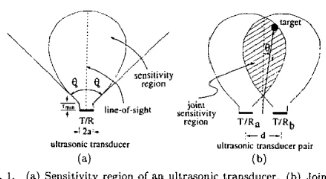
(b)

Fig. 1. (a) Sensitivity region of an ultra~onic transducer. (b) Joint

In our system, two identical ultrasonic transducers a and b w i t h center-to-center separation d are employed to im- prove the angular resolution of a single transducer. The

transducers can operate both as transmitter and receiver to detect echo signals reflected from targets nithin their joint sensitivity region (Fig. 1).

The targets used in this study are plane (P), corner (C), acute corner (AC), edge

(E)

and cylinder (CY) (Fig. 2 ) . Since the wavelength of operation (A E

8.6

mm at fo =

40 kHz) is much larger than the typical roughness of surfaces encountered in laboratory environments, targets in these environments reflect acoustic beams specularly, like a mirror. Detailed physical reflection models of these targets are provided in 121. In the following,

&.,

&,

Aob,

and Abo denote the maximum values of the sonar echo signals, and t,,, t b b , tab, and tba denote the T O F readings

extracted from these signals. The first index in the sub- script indicates the transmitting transducer, the second index denotes the receiver.

sensitivity region of a pair of ultra~onic transducers.

In commonly used T O F systems, an echo is produced when the transmitted pulse encounters an object and a

range valuer = ctJ2 is produced when the echo amplitude first exceeds a preset threshold level T at time to back at

the receiver. Here, to is the

TOF

and c is the speed of sound in air.

It

is observed that the echo amplitude decreases with in- creasing target range (.) and absolute value of the target azimuth

(161).

The echo amplitude falls below T when 16'1

>

tl,, which is related t o the aperture radius a and the reso- nance frequency fo of the transducer by

8,

= sin-'

(*>.

61c

PLANE CORNER ACUTE CORNER EDGE CYLINDER

Fig. 2. Horizontal cross sections of the targets differentiated

111.

TARGET DIFFERENTIATION

ALGORITHM

The

TDA

has its

roots

in the

P/C

differentiation

al-

gorithm developed in [l] based on the idea of exploiting amplitude differentials in resolving target type. In [Z], it is extended t o include other target primitives using both amplitude and T O F differentials:

i f [toa(Q) - t,b(Q)]

>

ktut and [ t b b ( O ) - t b . ( Q ) ]

>

ktut then A C

else if [Aae(a) - A,b(Q)]

>

k A U A and [Abb(a)

-

Ab,(a)]

>

~ A U A then P

B. Ayrulu and B. Banhan are with the Department of Electri- cal and Electronics Engineering, Bilkent University, 06533 Bilkent, Ankara, Turkey. Email: (ayrulu, biliur}~ee.bilkent.edu.tr .

else if [ m a x { A . . ( o ) } - m a x ( A b b ( ~ ) ] ]

<

kaoa and

[max(Abb(a))-max{A,b(n))] < k A U A then

c

else E, CY or U

(2)

The k A ( k c ) is the number of amplitude

(TOF)

noise stan- dard deviations ua(ot) and is employed

as

a

safety margin to achieve robust differentiation. Differentiation is achiev- able only in those cases where the difference in amplitudes (TOFs) exceeds

k ~ u ~ ( k ~ u ~ ) .

If

this is not the case, a decision cannot be made and the target type remains unknown.

IV. DEMPSTER-SHAFER E V I D E N T I A L REASONISG In DS, each sensor’s opinion is tied to

a

belief measure or basic probability mass assignment (BPMA) using belief functions (31. These are set functions which assign numer- ical degrees of support on the basis of evidence, but also allow for the expression of ignorance.

A

frame of discern- ment,

n,

represents a finite universe of propositions and a

BPMA, m(.), maps the power set of to the interval [0,1]. The BPMA satisfies the conditions:

740)

= 0,

1

74.4) = 1 (1)

A c n

A

set with a non-zero BPMA is afocal element. The belief or total support that is assigned to a set or proposition .-I is obtained by summing the B P x f . 4 ~ over all subsets of .-I:

B e l ( A ) =

1 m ( B )

(2)

B Z A

The uncertainty i n the measurements of each sonar pair is represented by a belief function having target type or feature as a focal element with BPMA m ( . ) :

B F

=

{feature; m( feature)}.

The BPMA is the underlying function for decision making using DS. It is defined based on the TD.4 and is thus dependent on amplitude and TOF differentials such that the larger the differential, the larger the degree of belief. The BPMA is made to plane, corner, and acute corner as

m@),m(c),

and m(ac), respectively. The remain- ing belief represents ignorance, or undistributed probability mass, and is assigned to an ‘unknown’ target type as

The sequential combination of multiple bodies of evi- m(u) = 1 - [m@)

+

m(c)

+

m(ac)].

dence can be obtained for n sensor nodes

as:

B F

=

( ( ( B F I

CB BFz) CB B F 3 ) .

. .

CB

BF,)

(3)

where

C

Chh=fing,=O

m~(f,)mz(gj) represents conflict

v.

CONFLICT RESOLUTION THROUGH VOTING

Multi-sensor systems exploit sensor diversity t o acquire

a

wider view of

a

scene under observation. This diver-

A .

Drflerent Voting Schemes

In

SMV,

the votes are given equal weight and the group

decision is taken as the outcome with the largest number of votes. Although SMV provides fast and robust fusion in some problems, there exist some drawbacks that limit its usage. For example, when all outcomes receive equal votes, a group decision cannot be reached. Moreover, it does not take into account the distribution of the decisions of dissenting classifiers. To overcome these drawbacks, more sophisticated voting schemes assigning preference ordering and reliability measures over the possible target types can be employed. Total preference is taken as the sum of the products of preference order assigned to each target type and the reliability measure assigned to the corresponding sensor node [6].

A . 1 Reliability Measure Assignment

Assignment of belief to range and azimuth estimates is based on the observation that the closer the target is to the surface of the transducer, the more accurate is the range reading, and the closer the t,arget is to the line-of-sight of the transducer (0 = 0”), the more accurate is the azimuth estimate. Therefore, belief assignments to range and az-

imuth estimates can be made as follows:

Five different reliability measures are assigned to sensor node i which are different functional combinations of m ( r )

and m(8) 161. Their performances are compared.

VI. STATISTICAL PATTERN RECOGNITION T E C H N I Q U E S

An object coming from one of N classes is classified into

class

wj

if its vector representation x is in region

ni.

A

rule which partitions a space into regions

R,, i

= 1 , . .

.

,

N

is called a decision rule. Boundaries between regions are

decision surfaces. The p ( w i ) are the a priori Probabilities of an object belonging to class

w,,i

= 1 , ’ .

, N .

To classify an object with vector representation x , a posteriori prob- abilities p ( w i l x ) , i = 1,. . .

,

N can be compared and the object is classified to class wk according to Bayes mini-

mum emor rule:

p(wklx)

>

p(w,lx) for all i

#

k

=+

x E Rk ₍₆₎

Since these a posteriori probabilities are rarely known, they need t o be estimated. Using Bayes’ theorem

[ p ( w i l x )

=

P ( X l W i ) P ( W d ] : P(4

~ ( x I w k ) P ( w k )

>

P(XIwi)P(wi) for all

i

#

k

*

x E Ok

(7)

sity can give rise to conflicts, which must be resolved when the system information is combined to reach a group decision or to form a group value

or

estimate. Voting has the advantages of being computationally inexpensive and, t o a

certain degree, fault-tolerant

[4].

Its major drawback is the consistency problem of Arrow which states that there is no voting scheme for selecting from more than two alternatives

where p(xlwi) are the clascconditional

PDFs.

The set

of vector representations used t o estimate these class- conditional PDFs is called design or training set. The performance of any decision rule can be assessed in a different set of vector representations which is called the test set.

More generally, classification rules can he written as

(3)

where q, is a discriminant function. Therefore, discriminant functions can be replaced with

PDFs

for computational simplicity. Linear discriminant functions result+.in additional computational advantages.

A. Kernel Estimator

(KE)

K E

is a class of P D F estimator first proposed by Parzen in 1962 [7]. In

KE,

the class-conditional PDF estimates are of the form:

(9) where

x

is the d-dimensional rector at which the estimate

is being made and xj's, j = 1,. . .

,

n; are samples in the design set. In this equation, ni is the total number of sample points in class w,, h is called the spread or smooth- ing parameter or bandwidth of a KE, and K ( z ) is a kernel function which satisfies the conditions K ( z )

2 0

and

J

K ( z ) d z = 1. Usually, h is chosen as a function of n, such that lim,,,,, h(n;) = 0. There are various approaches to select h if a constant h is to be used [8].

B. k-Nearest-Neighbor ( k - N N ) Method

Let

k

be the number of patterns from a combined set which are nearest neighbors of a pattern x , arid

ki

of them come from class w,. Then a k-NN estimator for class w; can be defined as:

The pattern x is classified as belonging to class wnL if

k,,,

=

max;(k;).

Another interpretation of the k-NN estimator which re- lates it to the KE can be found in [9]. Let rk(x) be the Euclidean distance from x to the kth

N N

of x in the training set and p(x1w;) estimates are taken as

This estimator is referred as generalized k-NN estimator.

C. PDE

with

Normal

Models

' '

to be a d-variate normal such that

In this method, each class-conditional PDF is assumed

where

i

= 1 , .

. .

,

N ,

pi's and Xi's denote the class mean and covariance matrices, respectively. They must be estimated by using techniques such as the maximum likelihood estimator based on the design set [lo].

Normal models (NM) used with

PDE

are divided into two as heteroscedastic and homoscedastic models. In the homoscedastic NM, all class-covariance matrjces are equal (Xi = X for all

i

= l , . . . , N ) . Usually X is taken as

the weighted average of each class-covariance matrix estimate [ l l ] . In the heteroscedastic NM, different class- covariance matrices are used for each class.

D. Linear Discriminant Analysis

(LDA)

In LDA, discriminant functions q(x)'s are linear functions of zi such that q(x) = a,

+

C;=,

a;z; = aTz where z = (1,

x

~

is the augmented observation vector. The aim

)

~

of LDA is to find the weight vector a, based on the design set which consists of two class samples such that

i) aTzi

>

O1 whenever xi is a sample from class w1, and ii) aTzi

<

0, whenever xi is a sample from class w2. Although the generalization of LDA to

N

classes can be done in different ways, here we have chosen to use

N

-

1 two-class decision rules, each one separating Ri,

i

=

1 , .

.

.,

N - 1 from all

Rj

j = 1 , . . .

,

N ; j

#

i.

VII. FUZZY C-MEANS

CLUSTERING

( F C C ) FCC bas been developed by Dunn 1121 and extended by Bezdek. It minimizes the following objective function with respect to fuzzy membership p;j and cluster centers Vi:

c N

J,,, = x(~ij)'"

/I

Xj

-

Vi

I l l

(12) i=* j = ,

where

11

x

I I i =

xTAx. A is a d x d positive definite matrix which specifies the shape of the clusters, d is the dimension of the input patterns

Xj

( j = 1,. . .

,

N ) , N is the number of

patterns, and rn

>

1 is the weighting exponent for pij and controls the fuzziness of the resulting clusters. Usually, A is chosen as the d x d identity matrix which leads the definition

of Euclidean distance resulting in spherical clusters.

VIII. ARTIFICIAL NEURAL NETWORKS (ANN) ANNs have been widely used in

a

variety of applications [13]. They consist of an input layer, one or more hidden layers, and a single output layer, each comprised of

a number of neurons. ANNs have three distinctive char- acteristics: The model of each neuron includes a smooth nonlinearity, the hidden layers extract progressively more meaningful features, and the ANN exhibits a high degree of connectivity. Due to the presence of distributed form of nonlinearity and high connectivity, theoretical analysis of ANNs is difficult. ANNs are trained to compute the boundaries of decision regions in the form of connection weights and biases by using training algorithms such as

back-propagation (BP) and generating-shrinking (GS). A. Preprocessing of the Input Signals

A . l Fourier Transform (FT) defined as:

The discrete Fourier transform (DFT) of a signal f(n) is

where N is the length of the signal f(n). The DFT can be represented in matrix notation as

fl

= Ff where

f

is

an

N x 1 column vector,

F

is the N x N DFT matrix, and fl is the DFT o f f .

(4)

A.2

Fractional Fourier Transform (FRT) for

0 <

( a (

<

2

as

[14]

The ath-order

FRT

fa(.) of the function

f(u)

is-defihed

f.(u)

k

Irn

K,(u,u')f(u')du' (14)

-m

~ ~ ( u , " ' )

C.

.a, exp [ j z ( Z c o t e

-

2 u u ' c s c o

+

u'2cotn)I (15)

where

The kernel K , ( u , u ' ) approaches 6(u - U') and 6(u

+

U ' )

as a approaches

0

and f-2, respectively, and are defined

as

such a t these values. The FRT reduces to the ordinary FT

when a = 1 and is linear and index additive; that is, the ai th-order

FRT

of the asth-order FRT of a function equals the (al

+

a2)th-order FRT. With a similar notation as in the case of DFT, the ath-order discrete fractional Fourier transform (DFRT) o f f , denoted

fa,

can be expressed as

fa

= F a f where Fa is the

N

x

h'

DFRT matrix which corresponds to the ath power of the ordinary DFT matrix F .

A.3 Hartley Transform (HT)

HT

1151 is another widely-used technique in signal processing applications 1151. The discrete Hartley transform (DHT) of a signal f(n) is defined as:

A 1 N - l

H ( k ) = 'H{f(n)} = f ( n ) cas ( Z n k ) (17)

A

where cas(z) = cos(z)

+

sin(z) and

N

is the length of the signal f(n). There is a close relationship between DFT and DHT such that if the DFT

of

a signal f(n) is expressed as F ( k ) = F ~ ( k ) - - j F l ( k ) , then its DHT is related to the real and imaginary parts of the DFT by

H ( k )

= F*(k)

+

F l ( k ) . The DHT can also be represented in matrix notation as hl

=

H f where f is an N x 1 column vector, H is the

N x N DHT matrix, and hl is the DHT o f f . A.4 Wavelet Transform (WT)

The discrete wavelet transform (DWT) of a function

k=-m j = O k=-m

where c ( k ) = < f ( t ) , r p k ( t ) > =

J f ( t ) v k ( t ) d t

and d ( j , k ) =

<

f(t),&*(t) > = J f ( t ) $ j , k ( t ) d t . The coefficients correspond to the DWT of signal f ( t ) . These coefficients completely describe the original signal and can be used in a way similar to Fourier series coefficients. The procedure

of

finding the DWT coefficients can be summarized as:

{ c ( k ) } Z - ,

and { d ( j ,

k)}j,o,k.-m

m,m

M-1

c1(k)

=

h(m

- Zk)Cj+l(rn) (19)

lll=O

H e r e , k = 0 , 1 ; . . , 2 J N - l where

N

isthenumberofsam- ples

of

the original signal that should be

a

power

of 2.

In these equations, h ( n ) , n = 0,.

.

' ,

A4

- 1 is a low-pass filter called the scaling filter and g(n) is

an

high-pass fil-

ter called the wavelet filter related to the scaling filter by

g ( n ) = (-l)"h(Af

-

1 -

n ) ,

n =

O,...,M

-

1. Usually, c,(k)'s are taken as the samples of the original signal.

A.5 Self Organizing Feature Map

Self organizing ANNs are obtained by unsupervised learning algorithms that have the ability to form internal representation of the network that model the underlying structure of the input data without supervision. These networks are commonly used to solve the scaling prohleni encountered in supervised learning procedures. It is possible to achieve best results with these networks as feature extractors prior to a linear classifier or a supervised learning process 1131. hlost commonly used algorithm for generating these networks is Kohonen's self organizing feature- mapping algorithm

(IiSOFhl)

(171 in which the weights are adjusted from the input layer to the output layer. The output neurons are interconnected with local connections and are geonietrically organized in one, two, three, or ercn higher dimensions.

1 s . E X P E R I M E N T A L S T U D I E S

Panasonic transducers with aperture radius a = O.G5 cm,

resonance frequency j o = 40 kHz, and

8,

% 54" 1131

are used (Fig. 1) with a center-to-center separation of d = 25 cm. The sensing unit is mounted on a stepper mi-

tor with step size 1.8" whose motion is controlled through the parallel port of a

PC.

Data acquisition is through a 12- bit 1 MHz

PC

A/D card. Starting a t the transmit time, 10,000 samples of each echo signal are collected and thresh- olded. The amplitude information is extracted by finding the maximum value of the signal after the threshold is ex- ceeded.

The targets employed in this study are: cylinders with radii

2.5,

5.0 and 7.5 cm, a planar target, a corner, an edge of 8, = go", and an acute corner of 8, = GOo. Amplitude and

TOF

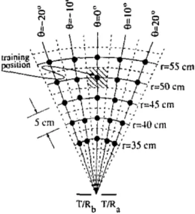
patterns of these targets are collected with the sensing unit described above at 25 different training locations

(.,e)

for each target (Fig. 3). T h e target primitive located at range T and azimuth 8 is scanned by the sensing

unit for scan angle -52"

5

a

5

52" with 1.8" increments.

For

given scan range and motor step size, 58 (=

s)

angular samples of each of amplitude and T O F patterns

[Am(a), Abb(a), Aob(a), & ( a ) ; tm(a), tbb(a), tab(a),

tba(a)] are acquired at each target location. Four similar sets of scans are collected for each target a t each location, resulting in 700

(=

4 data sets x 25 locations x 7 target types) sets of signals to construct the training data. This training data is used in statistical pattern recognition techniques, LDA,

FCC,

and ANNs.

Two different sets of test data are constructed to assess and compare the performances of the different classification and fusion techniques. For test data I, each target is placed in turn in each of the 25 training positions in Fig. 3.

(5)

d , o ,d ,

I< ,,.

T/Rb TIRa

Fig. 3. Discrete network training localions.

Four sets of patterns are collected for each combination of target type and location, again resulting in 700 sets of patterns. While collecting test data 11, targets are situated at randomly generated locations within the area shown in Fig. 3, not necessarily corresponding to one of the 25 grid locations.

Initially, the TD.A is employed at each angular step to classify and localize the target. Then, DS and various voting schemes are used to fuse decisions made at each of the

58 angular steps to reach a single decision for a pattern set. Weighted averages of the 58 range and azimuth estimates in a pattern set are calculated to find the range and the azimuth of the target. In DS, these weights are the belief values assigned to range and azimuth estimates at each angular step. In SMV, these weights are taken as one for both range and azimuth at each angular step. In voting schemes including preference ordering and reliability measures, reliabilities assigned at each angular step are used as weights. In this case, preference orders are taken as the belief values assigned to each target a t each angular step.

In statistical pattern recognition techniques, LDA, and FCC, three different training (design) sets are constructed using training data consisting of different vector representations. In each design set, seven classes each with 100 vector representations exist. These are:

'"'I'

..:[...I.,. A b * ( " ] . A - b ' y a (-1. in.ial. l b b I - l . ' * + ) p a

I'

..:[...i.,

-

A . * ( ~ l . l b l l ' l - A b s ( - ) . L D P I * . ) - .l''L.t Lbb''1 -%.'a)

-9: [lA&, - A & ~ . = l ! l A b b ~ . = l

-

A b a ~ * l l . l&*l.=l- * * & ( l ) l + l . 4 d - I - *b.(nl

I'

lh*'-l - t.b(allllbb'al -%*(")I. l I a e ( o / 1 - * d i ~ ) l + l t h b ' - )

-

I b * l ~ l l The first vector representation x1 is taken as the raw patterns without any processing, except for averaging the cross terms which should ideally be equal. The second vector representation xz has been motivated by the TDA. The third vector representation XQ is motivated by the differ-

ential terms which are used to assign belief values to the targets classified by the TDA [2].

Thirdly, ANNs are employed. Performance of ANNs is affected by the choice of parameters related to the network structure, training algorithm, and input signals, as well as

parameter initialization. We considered samples of the following different signal representations as alternative inputs to the ANNs: X l , x2, x3 DWT of xl, x2, XQ a t different resolutions j DFT of x i , X z , x 3 DFRT of xlr x2, xQ at different orders a DHT of X ~ , X Z , X Q

Features of xi, x2, x3 extracted by KSOFM

The first three input signal representations are the same vector representations used above for statistical pattern recognition techniques, LDA, and

FCC.

In this case, they have been used both in their raw form and after taking their DFT, DFRT, DHT, and DWT, as well as after feature extraction by KSOFM. The ath-order DFRT of these three input signal representations for a values varying from

0.05 to 0.95 with 0.05 increments are used. DWT of each signal representation a t different resolutions j are used. Fi- nally. the features extracted by using KSOFM are used as

input signals both prior to ANNs and linear classifiers. Initially, ANNs are trained by using BP to classify and localize these target types. Next, modular AXNs for each type of input signal have been implemented in which three separate networks for target type, range, and azimuth, each trained with

BP,

are employed. ANNs using the same input signal representations are also trained with the GS al-

gorithm. This algorithm can he applied to target classification but not localization [SI.

To make a comparison of all differentiation and fusion techniques employed in this study, highest percentages of correct classification obtained with each method are given in Table

X.

With the TDA and the fusion techniques based on this algorithm (DS, and various voting schemes) which do not use training data, only three of the target types employed in this study (P, C, and AC) can be differentiated. However, all targets can be differentiated with the other methods. The fact that the other methods are able t o distinguish all target types indicates that they must be

making more effective use of the available data than the TDA. Statistical pattern recognition techniques, LDA, and

FCC cannot be used for target localization, unlike all of the other methods. The highest percentages of correct classification is 100% and is obtained with non-modular ANN trained with

BP

employing the DFRT. However, best lo-

1,calization is achieved with the modular ANN trained with B P employing the DWT. The lowest percentage of correct classification is 61% and is obtained with the TDA. For most cases, vector representation XI gives the best re-

sults, followed by x~ and x ~ . Note that different vector representations are not applicable to TDA and fusion techniques based on this algorithm since they determine the target type by using differential signal xz obtained by us-

ing original signal x1 and they assign belief values to their decisions using XQ. For most cases, the results obtained

with test data

I

are the best for all methods except the TDA and the fusion techniques based on this algorithm. However, the gap between the results of test data I and I1 is higher for statistical pattern recognition techniques and LDA than that for all other methods.

(6)

raw signal DWT DFT DHT KSOFM DFRT

KSOFM with linear classifier (6)

TABLE I:

OVERVIEW OF T H E METHODS COMPARED, T H E TARGET T Y P E S ENCLOSED IN BRACES CAN B E RESOLVED ONLY

95 (95) (951 79/89(73/95) not Ptored 98 (99) [97] 71/90(80/92) 97 (98) (971 64/86(72/94) 99 (97) (971 67/84(62/84) 7R (76) 1131 24/69(21/66) 100 (98) 1971 75/~3(68/8fi)