Optimizing nonzero-based sparse matrix partitioning models via reducing latency

Contents lists available atScienceDirect

J. Parallel Distrib. Comput.

journal homepage:www.elsevier.com/locate/jpdc

Optimizing nonzero-based sparse matrix partitioning models via

reducing latency

✩

Seher Acer

,

Oguz Selvitopi

,

Cevdet Aykanat

∗

Bilkent University, Computer Engineering Department, 06800, Ankara, Turkey

h i g h l i g h t s

• Optimizing fine-grain hypergraph model to reduce bandwidth and latency. • Optimizing medium-grain hypergraph model to reduce bandwidth and latency. • Message net concept to encapsulate minimization of total message count. • Practical enhancements to establish a trade-off between bandwidth and latency. • Significant performance improvements validated on nearly one thousand matrices.

a r t i c l e i n f o

Article history:

Received 22 November 2017 Received in revised form 18 May 2018 Accepted 5 August 2018

Available online 18 August 2018

Keywords:

Sparse matrix

Sparse matrix–vector multiplication Row–column-parallel SpMV Load balancing Communication overhead Hypergraph Fine-grain partitioning Medium-grain partitioning Recursive bipartitioning a b s t r a c t

For the parallelization of sparse matrix–vector multiplication (SpMV) on distributed memory systems, nonzero-based fine-grain and medium-grain partitioning models attain the lowest communication vol-ume and computational imbalance among all partitioning models. This usually comes, however, at the expense of high message count, i.e., high latency overhead. This work addresses this shortcoming by proposing new fine-grain and medium-grain models that are able to minimize communication volume and message count in a single partitioning phase. The new models utilize message nets in order to encapsulate the minimization of total message count. We further fine-tune these models by proposing delayed addition and thresholding for message nets in order to establish a trade-off between the conflicting objectives of minimizing communication volume and message count. The experiments on an extensive dataset of nearly one thousand matrices show that the proposed models improve the total message count of the original nonzero-based models by up to 27% on the average, which is reflected on the parallel runtime of SpMV as an average reduction of 15% on 512 processors.

© 2018 Elsevier Inc. All rights reserved.

1. Introduction

Sparse matrix partitioning plays a pivotal role in scaling applica-tions that involve irregular sparse matrices on distributed memory systems. Several decades of research on this subject led to elegant combinatorial partitioning models that are able to address the needs of these applications.

A key operation in sparse applications is the sparse matrix– vector multiplication (SpMV), which is usually performed in a repeated manner with the same sparse matrix in various itera-tive solvers. The irregular sparsity pattern of the matrix in SpMV necessitates a non-trivial parallelization. In that sense, graph and

✩ This work was supported by The Scientific and Technological Research Council of Turkey (TUBITAK) under Grant EEEAG-114E545. This article is also based upon work from COST Action CA 15109 (COSTNET).

∗

Corresponding author.

E-mail addresses:acer@cs.bilkent.edu.tr(S. Acer),reha@cs.bilkent.edu.tr (O. Selvitopi),aykanat@cs.bilkent.edu.tr(C. Aykanat).

hypergraph models prove to be powerful tools in their immense ability to represent SpMV with the aim of optimizing desired parallel performance metrics. We focus on the hypergraph models as they correctly encapsulate the total communication volume in SpMV [6,7,13,15] and the proposed models in this work rely on hypergraphs.

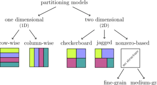
Among various hypergraph models, the fine-grain hypergraph model [8,10] achieves the lowest communication volume and the lowest imbalance on computational loads of the processors [10]. Since the nonzeros of the matrix are treated individually in the fine-grain model, the nonzeros that belong to the same row/ column are more likely to be scattered to multiple processors compared to the other models. This may result in a high message count and hinder scalability. The fine-grain hypergraphs have the largest size for the same reason, causing this model to have the highest partitioning overhead. The recently proposed medium-grain model [19] alleviates this issue by operating on groups of nonzeros instead of individual nonzeros. The partitioning overhead

https://doi.org/10.1016/j.jpdc.2018.08.005 0743-7315/©2018 Elsevier Inc. All rights reserved.

of the medium-grain model is significantly lower than that of the fine-grain model, while these two models achieve comparable communication volume. The fine-grain and medium-grain models are referred to as based models as they obtain nonzero-based matrix partitions, the most general possible [24].

Although the nonzero-based models attain the lowest commu-nication volume, the overall commucommu-nication cost is not determined by the volume only, but better formulated as a function of multiple communication cost metrics. Another important cost metric is the total message count, which is not only overlooked by both the fine-grain and medium-grain models, but also exacerbated due to having nonzero-based partitions. Note that among the two basic components of the communication cost, the total communication volume determines the bandwidth component and the total mes-sage count determines the latency component.

In this work, we aim at addressing the latency overheads of nonzero-based partitioning models. Our contributions can be sum-marized as follows:

•

We propose a novel fine-grain model to simultaneously re-duce the bandwidth and latency costs of parallel SpMV.

•

We propose a novel medium-grain model to simultaneously reduce the bandwidth and latency costs of parallel SpMV.

•

We utilize the message net concept [21] within the recursive bipartitioning framework to incorporate the minimization of the latency cost into the partitioning objective of these two models. Message nets aim to group the matrix nonzeros and/or the vector entries in the SpMV that necessitate a message together.

•

We also propose two enhancements, delayed addition and thresholding for message nets, to better exploit the trade-off between the bandwidth and latency costs for the proposed models.

•

We conduct extensive experiments on nearly one thousand matrices and show that the proposed models improve the total message count of the original nonzero-based models by up to 27% on the average, which is reflected on the parallel runtime of SpMV as an average reduction of 15% on 512 processors.

The remainder of the paper is organized as follows. Section2

gives background on parallel SpMV, performance cost metrics, the fine-grain model, recursive bipartitioning, and the medium-grain model. Sections 3 and 4 present the proposed fine-grain and medium-grain models, respectively. Section5describes practical enhancements to these models. Sections 6 and 7 give the ex-perimental results and related work, respectively, and Section8

concludes. 2. Preliminaries

2.1. Row–column-parallel SpMV

We consider the parallelization of SpMV of the form y

=

Ax with a nonzero-based partitioned matrix A, where A

=

(ai,j) is an

nr

×

ncsparse matrix with nnznonzero entries, and x and y are

dense vectors. The ith row and the jth column of A are, respectively, denoted by riand cj. The jth entry of x and the ith entry of y are,

respectively, denoted by xjand yi. LetAdenote the set of nonzero

entries in A, that is,A

= {

ai,j

:

ai,j

̸=

0

}

. LetXandY, respectively,

denote the sets of entries in x and y, that is,X

= {

x1, . . . ,xnc

}

andY

= {

y1, . . . ,ynr

}

. Assume that there are K processors in the parallel system denoted by P1, . . . ,PK. LetΠK(A)

= {

A1, . . . ,AK

}

,

ΠK(X)

= {

X1, . . . ,XK

}

, andΠK(Y)

= {

Y1, . . . ,YK

}

denote K -way

partitions ofA,X, andY, respectively.

Given partitionsΠK(A),ΠK(X), andΠK(Y), without loss of

gen-erality, the nonzeros inAkand the vector entries inXkandYkare

Algorithm 1: Row–column-parallel SpMV as performed by pro-cessor Pk.

Require: A_k,X_k

▷Pre-communication phase — expands on x-vector entries Receive the needed x-vector entries that are not inXk

Send the x-vector entries inX_kneeded by other processors ▷Computation phase

y(k)_i

←

y(k)_i

+

ai,jxjfor each ai,j

∈

Ak

▷Post-communication phase — folds on y-vector entries Receive the partial results for y-vector entries inYkand

compute yi

←

∑

y(_iℓ)for each partial result y(_iℓ) Send the partial results for y-vector entries not inY_k return Y_k

assigned to processor Pk. For each ai,j

∈

Ak, Pkis held responsible

for performing the respective multiply-and-add operation y(k)_i

←

y(k)_i

+

ai,jxj, where y(k)i denotes the partial result computed for yiby

Pk. Algorithm1displays the basic steps performed by Pkin parallel

SpMV for a nonzero-based partitioned matrix A. This algorithm is called the row–column-parallel SpMV [22]. In this algorithm, Pkfirst

receives the needed x-vector entries that are not inX_kfrom their owners and sends its x-vector entries to the processors that need them in a pre-communication phase. Sending xjto possibly multiple

processors is referred to as the expand operation on xj. When Pkhas

all needed x-vector entries, it performs the local SpMV by comput-ing y(k)_i

←

y(k)_i

+

ai,jxjfor each ai,j

∈

Ak. Pkthen receives the partial

results for the y-vector entries inY_kfrom other processors and sends its partial results to the processors that own the respective y-vector entries in a post-communication phase. Receiving partial result(s) for yifrom possibly multiple processors is referred to as

the fold operation on yi. Note that overlapping of computation and

communication is not considered in this algorithm for the sake of clarity.

2.2. Performance cost metrics

In this section, we describe the performance cost metrics that are minimized by the proposed models and formulate them on given K -way partitionsΠK(A), ΠK(X), and ΠK(Y). Let e(Pk

,

Pℓ)

denote the set of x-vector entries sent (expanded) from processor Pkto processor Pℓduring the pre-communication phase. Similarly,

let f (Pk

,

Pℓ) denote the set of partial results for y-vector entries sent

(folded) from Pkto Pℓduring the post-communication phase. That

is,

e(Pk

,

Pℓ)

= {

xj

:

xj

∈

Xkand

∃

at,j

∈

Aℓ

}

and

f (Pk

,

Pℓ)

= {

y(k)_i

:

yi

∈

Yℓand

∃

ai,t

∈

Ak

}

.

(1) Total communication volume is equal to the sum of the sizes of all messages transmitted during pre-communication and post-communication phases and formulated as

∑

k

∑

ℓ

|

e(Pk

,

Pℓ)

| + |

f (Pk

,

Pℓ)

|

.

Total message count is equal to the total number of messages and formulated as

|{

(k

, ℓ

)

:

e(Pk

,

Pℓ)

̸= ∅}| + |{

(k

, ℓ

)

:

f (Pk

,

Pℓ)

̸= ∅}|

.

Computational imbalance is equal to the ratio of the maximum to the average amount of computation performed by a processor mi-nus one. Since the amount of computation in SpMV is proportional to the number of nonzeros, computational imbalance is formulated

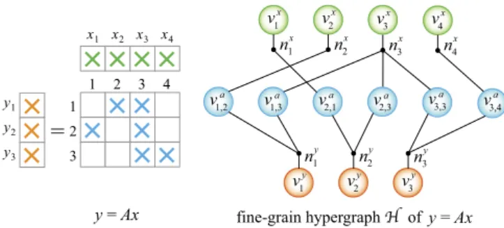
Fig. 1. A sample y=Ax and the corresponding fine-grain hypergraph.

as maxk

|

Ak

|

|

A

|

/

K

−

1

.

For an efficient row–column-parallel SpMV, the goal is to find partitionsΠK(A),ΠK(X) andΠK(Y) that achieve low

communi-cation overheads and low computational imbalance. Existing fine-grain [9] and medium-grain [19] models, which are, respectively, described in Sections2.3and2.5, meet this goal partially by only minimizing the bandwidth cost (i.e., total communication volume) while maintaining balance on the computational loads of proces-sors.

2.3. Fine-grain hypergraph model

In the fine-grain hypergraphH

=

(V

,

N), each entry inA,X, andYis represented by a different vertex. Vertex setVcontains a vertex

v

a

i,jfor each ai,j

∈

A, a vertex

v

jxfor each xj

∈

X, and a vertex

v

y

i for each yi

∈

Y. That is,

V

= {

v

_ia_,j

:

ai,j

̸=

0

} ∪ {

v

1, . . . , vx nxc

} ∪ {

v

y

1, . . . , vy nr

}

.

v

a

i,jrepresents both the data element ai,jand the computational

task yi

←

yi

+

ai,jxjassociated with ai,j, whereas

v

xjand

v

y

i only

rep-resent the input and output data elements xjand yi, respectively.

The net setN contains two different types of nets to represent the dependencies of the computational tasks on x- and y-vector entries. For each xj

∈

Xand yi

∈

Y,N, respectively, contains the

nets nx_jand ny_i. That is,

N

= {

nx₁

, . . . ,

nx_nc

} ∪ {

ny₁

, . . . ,

ny_nr

}

.

Net nx

jrepresents the input dependency of the computational tasks

on xj; hence, it connects the vertices that represent these tasks and

v

x j. Net n

y

i represents the output dependency of the computational

tasks on yi; hence, it connects the vertices that represent these

tasks and

v

y_i. The sets of vertices connected by nx_j and ny_i are, respectively, formulated as

Pins(nx_j)

= {

v

_jx

} ∪ {

v

_ta_,j

:

at,j

̸=

0

}

and

Pins(ny_i)

= {

v

_iy

} ∪ {

v

_ia_,t

:

ai,t

̸=

0

}

.

Hcontains nnz

+

nc

+

nrvertices, nc

+

nrnets and 2nnz

+

nc

+

nr

pins.Fig. 1displays a sample SpMV instance and its corresponding fine-grain hypergraph. InH, the vertices are assigned the weights that signify their computational loads. Hence,

w

(

v

a

i,j)

=

1 for each

v

a

i,j

∈

V as

v

i,j represents a single multiply-and-add operation,

whereas

w

(

v

x j)

=

w

(

v

y

i)

=

0 for each

v

jx

∈

Vand

v

y

i

∈

Vas they do

not represent any computation. The nets are assigned unit costs, i.e., c(nx_j)

=

c(ny_i)

=

1 for each nx_j

∈

Nand ny_i

∈

N.

A K -way vertex partitionΠK(H)

= {

V1, . . . ,VK

}

can be

de-coded to obtainΠK(A),ΠK(X), andΠK(Y) by assigning the entries

represented by the vertices in partVkto processor Pk. That is,

A_k

= {

ai,j

:

v

ia,j

∈

Vk

}

,

X_k

= {

xj

:

v

xj

∈

Vk

}

,

and

Y_k

= {

yi

:

v

y i

∈

Vk

}

.

LetΛ(n) denote the set of the parts connected by net n inΠK(H),

where a net is said to connect a part if it connects at least one vertex in that part. Let

λ

(n) denote the number of parts connected by n, i.e.,

|

Λ(n)

|

. A net n is called cut if it connects at least two parts, i.e.,

λ

(n)

>

1, and uncut, otherwise. The cutsize ofΠK(H) is defined

as

cutsize(ΠK(H))

=

∑

n∈N

c(n)(

λ

(n)

−

1)

.

(2)

Consider cut nets nx j and n

y

i inΠK(H) and assume that

v

jx

, v

y i

∈

Vk. The cut net nxj necessitates sending (expanding) of xjfrom Pk

to the processors that correspond to the parts inΛ(nx

j)

− {

Vk

}

in

the pre-communication phase. Hence, it can be said that if nx j is

cut, then

v

x

j incurs a communication volume of

λ

(nxj)

−

1. The cut

net ny_i, on the other hand, necessitates sending (folding) of the partial results from the processors that correspond to the parts in

Λ(ny_i)

− {

Vk

}

to Pk, which then sums them up to obtain yi. Hence,

it can be said that if ny_i is cut, then

v

y_i incurs a communication volume of

λ

(ny_i)

−

1. Since each cut net n increases the cutsize by

λ

(n)

−

1

>

0, cutsize(ΠK(H)) is equal to the sum of the volume

in pre- and post-communication phases. Therefore, minimizing cutsize(ΠK(H)) corresponds to minimizing the total

communica-tion volume in row–column-parallel SpMV.

The contents of the messages sent from Pkto Pℓin the pre- and

post-communication phases in terms of a partitioned hypergraph are, respectively, given by

e(Pk

,

Pℓ)

= {

xj

:

v

xj

∈

VkandVℓ

∈

Λ(nxj)

}

and

f (Pk

,

Pℓ)

= {

y (k) i

:

v

y i

∈

VℓandVk

∈

Λ(n y i)

}

.

(3) Note the one-to-one correspondence between sparse matrix and hypergraph partitionings in determining the message contents given by Eqs.(1)and(3).

InΠK(H), the weight W (Vk) of partVkis defined as the sum

of the weights of the vertices inV_k, i.e., W (Vk)

=

∑

v∈Vk

w

(

v

), which is equal to the total computational load of processor Pk.

Then, maintaining the balance constraint W (Vk)

≤

Wavg(1

+

ϵ

)

,

for k

=

1

, . . . ,

K

,

corresponds to maintaining balance on the computational loads of the processors. Here, Wavg and

ϵ

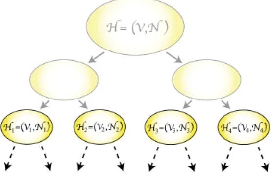
denote the average part weight

and a maximum imbalance ratio, respectively. 2.4. Recursive bipartitioning (RB) paradigm

In RB, a given domain is first bipartitioned and then this bipar-tition is used to form two new subdomains. In our case, a domain refers to a hypergraph (H) or a set of matrix and vector entries (A,X,Y). The newly-formed subdomains are recursively biparti-tioned until K subdomains are obtained. This procedure forms a hypothetical full binary tree, which contains

⌈

log K

⌉ +

1 levels. The root node of the tree represents the given domain, whereas each of the remaining nodes represents a subdomain formed during the RB process. At any stage of the RB process, the subdomains represented by the leaf nodes of the RB tree collectively induce a partition of the original domain.

The RB paradigm is successfully used for hypergraph parti-tioning. Fig. 2illustrates an RB tree currently in the process of partitioning a hypergraph. The current leaf nodes induce a four-way partitionΠ4(H)

= {

V1,V2,V3,V4

}

and each node in the RB

Fig. 2. The RB tree during partitioningH=(V,N). The current RB tree contains four leaf hypergraphs with the hypergraph to be bipartitioned next beingH₁ =

(V1,N1).

two new subhypergraphs after each RB step, the cut-net splitting technique is used [7] to encapsulate the cutsize in(2). The sum of the cutsizes incurred in all RB steps is equal to the cutsize of the resulting K -way partition.

2.5. Medium-grain hypergraph model

In the medium-grain hypergraph model, the setsA,XandYare partitioned into K parts using RB. The medium-grain model uses a mapping for a subset of the nonzeros at each RB step. Because this mapping is central to the model, we focus on a single bipartitioning step to explain the medium-grain model. Before each RB step, the nonzeros to be bipartitioned are first mapped to their rows or columns by a heuristic and a new hypergraph is formed according to this mapping.

Consider an RB tree for the medium-grain model with K′

leaf nodes, where K′

<

K , and assume that the kth node from the left is to be bipartitioned next. This node representsAk,Xk, andYk

in the respective K′

-way partitions

{

A1, . . . ,A_{K ′}

}

,

{

X1, . . . ,X_{K ′}

}

, and

{

Y1, . . . ,Y_{K ′}

}

. First, each ai,j

∈

Akis mapped to either ri or

cj, where this mapping is denoted by map(ai,j). With a heuristic,

ai,j

∈

Akis mapped to ri if rihas fewer nonzeros than cjinAk,

and to cjif cjhas fewer nonzeros than riinAk. After determining

map(ai,j) for each nonzero inAk, the medium-grain hypergraph

Hk

=

(Vk

,

Nk) is formed as follows. Vertex setVkcontains a vertex

v

x

jif xjis inXkor there exists at least one nonzero inAkmapped to

cj. Similarly,Vkcontains a vertex

v

iyif yiis inYkor there exists at

least one nonzero inAkmapped to ri. Hence,

v

xjrepresents xjand/or

the nonzero(s) assigned to cj, whereas

v

yi represents yiand/or the

nonzero(s) assigned to ri. That is,

V_k

= {

v

_jx

:

xj

∈

Xkor

∃

at,j

∈

Aks.t. map(at,j)

=

cj

} ∪

{

v

y_i

:

yi

∈

Ykor

∃

ai,t

∈

Aks.t. map(ai,t)

=

ri

}

.

Besides the data elements, vertex

v

x j/

v

y

i represents the group of

computational tasks associated with the nonzeros mapped to them, if any.

The net set Nk contains a net nxj ifAk contains at least one

nonzero in cj, and a net nyi ifAkcontains at least one nonzero in

ri. That is,

N_k

= {

nx_j

: ∃

at,j

∈

Ak

} ∪ {

nyi

: ∃

ai,t

∈

Ak

}

.

nx

jrepresents the input dependency of the groups of computational

tasks on xj, whereas nyi represents the output dependency of the

groups of computational tasks on yi. Hence, the sets of vertices

connected by nx jand n

y

i are, respectively, formulated by

Pins(nx

j)

= {

v

jx

} ∪ {

v

y

t

:

map(at,j)

=

rt

}

and

Pins(ny_i)

= {

v

y_i

} ∪ {

v

_tx

:

map(ai,t)

=

ct

}

.

Fig. 3. The nonzero assignments of the sample y = Ax and the corresponding

medium-grain hypergraph.

InH_k, each net is assigned a unit cost, i.e., c(nx_j)

=

c(ny_i)

=

1 for each nx

j

∈

Nand n y

i

∈

N. Each vertex is assigned a weight equal to

the number of nonzeros represented by that vertex. That is,

w

(

v

_jx)

= |{

at,j

:

map(at,j)

=

cj

}|

and

w

(

v

_iy)

= |{

ai,t

:

map(ai,t)

=

ri

}|

.

H_kis bipartitioned with the objective of minimizing the cutsize and the constraint of maintaining balance on the part weights. The resulting bipartition is further improved by an iterative refinement algorithm. In every RB step, minimizing the cutsize corresponds to minimizing the total volume of communication, whereas taining balance on the weights of the parts corresponds to main-taining balance on the computational loads of the processors.

Fig. 3 displays a sample SpMV instance with nonzero map-ping information and the corresponding medium-grain hyper-graph. This example illustrates the first RB step, hence,A1

=

A,

X₁

=

X,Y₁

=

Y, and K′

₌

k

=

1. Each nonzero in A is denoted by an arrow, where the direction of the arrow shows the mapping for that nonzero. For example, nx

3connects

v

3x,

v

y 1,

v

y 2, and

v

y 3since

map(a1,3)

=

r1, map(a2,3)

=

r2, and map(a3,3)

=

r3. 3. Optimizing fine-grain partitioning model

In this section, we propose a fine-grain hypergraph partitioning model that simultaneously reduces the bandwidth and latency costs of the row–column-parallel SpMV. Our model is built upon the original fine-grain model (Section 2.3) via utilizing the RB paradigm. The proposed model contains two different types of nets to address the bandwidth and latency costs. The nets of the original fine-grain model already address the bandwidth cost and they are called ‘‘volume nets’’ as they encapsulate the minimization of the total communication volume. At each RB step, our model forms and adds new nets to the hypergraph to be bipartitioned. These new nets address the latency cost and they are called ‘‘message nets’’ as they encapsulate the minimization of the total message count.

Message nets aim to group the matrix nonzeros and vector entries that altogether necessitate a message. The formation and addition of message nets rely on the RB paradigm. To determine the existence and the content of a message, a partition information is needed first. At each RB step, prior to bipartitioning the current hypergraph that already contains the volume nets, the message nets are formed using the K′

-way partition information and added to this hypergraph, where K′

is the number of leaf nodes in the current RB tree. Then this hypergraph is bipartitioned, which re-sults in a (K′

+

1)-way partition as the number of leaves becomes K′

₊

1 after bipartitioning. Adding message nets just before each bipartitioning allows us to utilize the most recent global partition information at hand. In contrast to the formation of the message nets, the formation of the volume nets via cut-net splitting requires only the local bipartition information.

3.1. Message nets in a single RB step

Consider an SpMV instance y

=

Ax and its corresponding fine-grain hypergraphH

=

(V

,

N) with the aim of partitioningHinto K parts to parallelize y

=

Ax. The RB process starts with bipartition-ingH, which is represented by the root node of the corresponding RB tree. Assume that the RB process is at the state where there are K′

leaf nodes in the RB tree, for 1

<

K′

<

K , and the hypergraphs corresponding to these nodes are denoted byH1, . . . ,HK ′from left

to right. LetΠK ′(H)

= {

V1, . . . ,VK ′

}

denote the K′-way partition

induced by the leaf nodes of the RB tree.Π_{K ′}(H) also induces K′

-way partitionsΠK ′(A),ΠK ′(X), andΠK ′(Y) of setsA,X, andY,

respectively. Without loss of generality, the entries inA_k,X_k, and Y_kare assigned to processor groupP_k. Assume thatH_k

=

(Vk

,

Nk)

is next to be bipartitioned among these hypergraphs.Hkinitially

contains only the volume nets. In our model, we add message nets toH_kto obtain the augmented hypergraphHM_k

=

(Vk

,

NkM). Let

Π(HM_k)

= {

V_k,L

,

V_k,R

}

denote a bipartition ofHM_k, where L and R in the subscripts refer to left and right, respectively.Π(HM_k) induces bipartitionsΠ(Ak)

= {

Ak,L

,

Ak,R

}

,Π(Xk)

= {

Xk,L

,

Xk,R

}

,

and Π(Yk)

=

{

Yk,L

,

Yk,R

}

onAk, Xk, and Yk, respectively. Let

P_k,LandP_k,Rdenote the processor groups to which the entries in

{

A_k,L

,

X_k,L

,

Y_k,L

}

and

{

A_k,R

,

X_k,R

,

Y_k,R

}

are assigned.

Algorithm2displays the basic steps of forming message nets and adding them to Hk. For each processor group Pℓ that Pk

communicates with, four different message nets may be added toHk: expand-send net, expand-receive net, fold-send net and

fold-receive net, respectively, denoted by se_ℓ, r_ℓe, sf_ℓ and r_ℓf. Here, s and r, respectively, denote the messages sent and received, the subscript

ℓ

denotes the id of the processor group communicated with, and the superscripts e and f , respectively, denote the expand and fold operations. These nets are next explained in detail.

•

expand-send net se

ℓ: Net seℓrepresents the message sent from

PktoPℓduring the expand operations on x-vector entries

in the pre-communication phase. This message consists of the x-vector entries owned byP_kand needed byP_ℓ. Hence, se

ℓconnects the vertices that represent the x-vector entries

required by the computational tasks inP_ℓ. That is, Pins(se_ℓ)

= {

v

_jx

:

xj

∈

Xkand

∃

at,j

∈

Aℓ

}

.

The formation and addition of expand-send nets are per-formed in lines 2–7 of Algorithm2. After bipartitioningHM_k, if se

ℓbecomes cut inΠ(HMk), bothPk,LandPk,Rsend a message

toP_ℓ, where the contents of the messages sent fromPk,L

andP_k,RtoP_ℓare

{

xj

:

v

jx

∈

Vk,Land at,j

∈

Aℓ

}

and

{

xj

:

v

x

j

∈

Vk,Rand at,j

∈

Aℓ

}

, respectively. The overall number of

messages in the pre-communication phase increases by one in this case sincePkwas sending a single message toPℓand

it is split into two messages after bipartitioning. If se_ℓbecomes uncut, the overall number of messages does not change since only one ofPk,LandPk,Rsends a message toPℓ.

•

expand-receive net r_ℓe: Net r_ℓe represents the message re-ceived by P_kfromP_ℓ during the expand operations on x-vector entries in the pre-communication phase. This message consists of the x-vector entries owned byP_ℓand needed by P_k. Hence, r_ℓeconnects the vertices that represent the compu-tational tasks requiring x-vector entries fromP_ℓ. That is, Pins(r_ℓe)

= {

v

a_t,j

:

at,j

∈

Akand xj

∈

Xℓ

}

.

The formation and addition of expand-receive nets are per-formed in lines 8–13 of Algorithm2. After bipartitioningHM_k, if r_ℓebecomes cut inΠ(HM_k), bothP_k,LandP_k,Rreceive a mes-sage fromP_ℓ, where the contents of the messages received byP_k,LandP_k,RfromP_ℓare

{

xj

:

v

ta,j

∈

Vk,Land xj

∈

Xℓ

}

and

{

xj

:

v

ta,j

∈

Vk,Rand xj

∈

Xℓ

}

, respectively. The overall number

Algorithm 2: ADD-MESSAGE-NETS. Require: H_k

=

(Vk

,

Nk),ΠK ′(A)

= {

A1, . . . ,AK ′

}

,ΠK ′(X)

=

{

X1, . . . ,XK ′

}

,ΠK ′(Y)

= {

Y1, . . . ,YK ′

}

. 1: N_kM

←

Nk ▷ Expand-send nets 2: for each xj

∈

Xkdo 3: for each at,j

∈

Aℓ̸=kdo 4: if se ℓ

/∈

NkMthen 5: Pins(se_ℓ)

← {

v

_jx

}

,N_kM

←

N_kM

∪ {

se_ℓ

}

6: else 7: Pins(se ℓ)

←

Pins(seℓ)

∪ {

v

xj

}

▷ Expand-receive nets 8: for each at,j

∈

Akdo 9: for each xj

∈

Xℓ̸=kdo 10: if r_ℓe

/∈

N_kMthen 11: Pins(re ℓ)

← {

v

at,j

}

,NkM

←

NkM

∪ {

rℓe

}

12: else 13: Pins(r_ℓe)

←

Pins(r_ℓe)

∪ {

v

_ta_,j

}

▷ Fold-send nets 14: for each ai,t

∈

Akdo 15: for each yi

∈

Yℓ̸=kdo 16: if sf_ℓ

/∈

N_kMthen 17: Pins(sf_ℓ)

← {

v

_ia_,t

}

,N_kM

←

N_kM

∪ {

sf_ℓ

}

18: else 19: Pins(sf_ℓ)

←

Pins(sf_ℓ)

∪ {

v

a i,t

}

▷ Fold-receive nets 20: for each yi

∈

Ykdo 21: for each ai,t

∈

Aℓ̸=kdo 22: if r_ℓf

/∈

N_kMthen 23: Pins(r_ℓf)

← {

v

_iy

}

,N_kM

←

N_kM

∪ {

r_ℓf

}

24: else 25: Pins(r_ℓf)

←

Pins(r_ℓf)

∪ {

v

_iy

}

26: return HM_k

=

(Vk

,

NkM)

of messages in the pre-communication phase increases by one in this case and does not change if re

ℓbecomes uncut.

•

fold-send net sf_ℓ: Net sf_ℓrepresents the message sent from P_ktoP_ℓduring the fold operations on y-vector entries in the post-communication phase. This message consists of the par-tial results computed byPkfor the y-vector entries owned by

P_ℓ. Hence, sf_ℓconnects the vertices that represent the compu-tational tasks whose partial results are required byP_ℓ. That is, Pins(sf_ℓ)

= {

v

a_i,t

:

ai,t

∈

Akand yi

∈

Yℓ

}

.

The formation and addition of fold-send nets are performed in lines 14–19 of Algorithm2. After bipartitioningHM_k, if sf_ℓ becomes cut inΠ(HM

k), bothPk,LandPk,Rsend a message to

P_ℓ, where the contents of the messages sent fromP_k,Land P_k,R toP_ℓare

{

y(k_i ,L)

:

v

a_i,t

∈

V_k,Land yi

∈

Yℓ

}

and

{

y(ki ,R)

:

v

a

i,t

∈

Vk,Rand yi

∈

Yℓ

}

, respectively. The overall number of messages in the post-communication phase increases by one in this case and does not change if sf_ℓbecomes uncut.

•

fold-receive net r_ℓf: Net r_ℓf represents the message received byPkfromPℓduring the fold operations on y-vector entries in

the post-communication phase. This message consists of the partial results computed byP_ℓfor the y-vector entries owned by P_k. Hence, r_ℓf connects the vertices that represent the y-vector entries for whichP_ℓproduces partial results. That is, Pins(r_ℓf)

= {

v

_iy

:

yi

∈

Ykand

∃

ai,t

∈

Aℓ

}

.

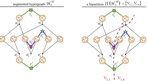
Fig. 4. A 5-way nonzero-based partition of an SpMV instance y=Ax.

Table 1

The messages communicated byP3in pre- and post-communication phases

be-fore and after bipartitioningHM

3. The number of messages communicated byP3

increases from 4 to 6 due to two cut message nets inΠ(HM₃).

RB state Phase Message Due to

BeforeΠ(HM 3) Pre P3sends{x3,x7}toP4 a5,3,a5,7 P3receives{x4,x5}fromP1 a2,4,a4,5 Post P3sends{y (3) 2 }toP2 a2,3,a2,4 P3receives{y(4)1 ,y (4) 4 }fromP4 a1,1,a4,1 AfterΠ(HM₃) Pre P3,Lsends{x3,x7}toP4 a5,3,a5,7 P3,Rreceives{x4,x5}fromP1 a2,4,a4,5 Post P3,Lsends{y2(3,L)}toP2 a2,3 P3,Rsends{y2(3,R)}toP2 a2,4 P3,Lreceives{y (4) 1 }fromP4 a1,1 P3,Rreceives{y(4)4 }fromP4 a4,1

The formation and addition of fold-receive nets are per-formed in lines 20–25 of Algorithm2. After bipartitioningHM

k,

if r_ℓfbecomes cut inΠ(HM_k), bothP_k,LandP_k,Rreceive a mes-sage fromP_ℓ, where the contents of the messages received by P_k,LandP_k,RfromP_ℓare

{

y_i(ℓ)

:

v

_iy

∈

V_k,Land ai,t

∈

Aℓ

}

and

{

y(_iℓ)

:

v

_iy

∈

V_k,Rand ai,t

∈

Aℓ

}

, respectively. The overall

num-ber of messages in the post-communication phase increases by one in this case and does not change if r_ℓfbecomes uncut. Note that at most four message nets are required to encapsulate the messages between processor groupsPkandPℓ. The message

nets inHM_k encapsulate all the messages that Pkcommunicates

with other processor groups. Since the number of leaf hypergraphs is K′,Pkmay communicate with at most K′

−

1 processor groups,

hence the maximum number of message nets that can be added to H_kis 4(K′

₋

1).

Fig. 4displays an SpMV instance with a 6

×

8 matrix A, which is being partitioned by the proposed model. The RB process is at the state where there are five leaf hypergraphsH1, . . . ,H5, and

the hypergraph to be bipartitioned next isH₃. The figure displays the assignments of the matrix nonzeros and vector entries to the corresponding processor groupsP1, . . . ,P5. Each symbol in the

figure represents a distinct processor group and a symbol inside a cell signifies the assignment of the corresponding matrix nonzero or vector entry to the processor group represented by that symbol. For example, the nonzeros inA₃

= {

a1,3,a1,7,a2,3,a2,4,a4,5,a4,7

}

,

x-vector entries inX3

= {

x3,x7

}

, and y-vector entries inY3

=

{

y1,y4

}

are assigned toP3. The left ofFig. 5displays the augmented

hypergraphHM

3 that contains volume and message nets. In the

fig-ure, the volume nets are illustrated by small black circles with thin lines, whereas the message nets are illustrated by the respective processor’s symbol with thick lines.

The messages communicated by P3 under the assignments

given inFig. 4are displayed at the top half ofTable 1. In the pre-communication phase,P3 sends a message toP4and receives a

message fromP1, and in the post-communication phase, it sends

a message toP₂and receives a message fromP₄. Hence, we add four message nets toH3: expand-send net se4, expand-receive net

re

1, fold-send net s

f

2, and fold-receive net r

f

4. InFig. 5, for example, r1e

connects the vertices

v

a

2,4and

v

a4,5since it represents the message

received byP₃fromP₁containing

{

x4,x5

}

due to nonzeros a2,4

and a4,5. The right ofFig. 5displays a bipartitionΠ(HM3) and the

messages thatP3,LandP3,Rcommunicate with the other processor

groups due toΠ(HM₃) are given in the bottom half ofTable 1. Since se

4and r1eare uncut, only one ofP3,LandP3,Rparticipates in sending

or receiving the corresponding message. Since sf₂is cut, bothP3,L

andP3,Rsend a message toP2, and since r4f is cut, bothP3,Land

P_3,Rreceive a message fromP₄.

In HM_k, each volume net is assigned the cost of the per-word transfer time, t_w, whereas each message net is assigned the cost of the start-up latency, tsu. Let

v

and m, respectively, denote the

number of volume and message nets that are cut inΠ(HM_k). Then, cutsize(Π(HM_k))

=

v

t_w

+

mtsu

.

Here,

v

is equal to the increase in the total communication volume incurred byΠ(HM

k) [7]. Recall that each cut message net increases

the number of messages thatPkcommunicates with the respective

processor group by one. Hence, m is equal to the increase in the number of messages thatP_kcommunicates with other processor groups. The overall increase in the total message count due to

Π(HM

k) is m

+

δ

, where

δ

denotes the number of messages

be-tweenPk,LandPk,R, and is bounded by two (empirically found to

be almost always two). Hence, minimizing the cutsize ofΠ(HM_k) corresponds to simultaneously reducing the increase in the total communication volume and the total message count in the re-spective RB step. Therefore, minimizing the cutsize in all RB steps corresponds to reducing the total communication volume and the total message count simultaneously.

After obtaining a bipartitionΠ(HM_k)

= {

V_k,L

,

V_k,R

}

of the aug-mented hypergraphHM

k, the new hypergraphsHk,L

=

(Vk,L

,

Nk,L)

andH_k,R

=

(Vk,R

,

Nk,R) are immediately formed with only volume

nets. Recall that the formation of the volume nets ofHk,LandHk,R

is performed with the cut-net splitting technique and it can be performed using the local bipartition informationΠ(HM_k). 3.2. The overall RB

After completing an RB step and obtainingHk,L andHk,R, the

labels of the hypergraphs represented by the leaf nodes of the RB tree are updated as follows. For 1

≤

i

<

k, the label of Hi

=

(Vi

,

Ni) does not change. For k

<

i

<

K′,Hi

=

(Vi

,

Ni)

becomesHi+1

=

(Vi+1,Ni+1). HypergraphsHk,L

=

(Vk,L

,

Nk,L)

and H_k,R

=

(Vk,R

,

Nk,R) become Hk

=

(Vk

,

Nk) andHk+1

=

(Vk+1,Nk+1), respectively. As a result, the vertex sets

correspond-ing to the updated leaf nodes induce a (K′

₊

1)-way partition

ΠK ′+1(H)

= {

V1, . . . ,VK ′+1

}

. The RB process then continues with

the next hypergraphH_k+2to be bipartitioned, which was labeled

withHk+1in the previous RB state.

We next provide the cost of adding message nets through Algo-rithm2in the entire RB process. For the addition of expand-send nets, all nonzeros at,j

∈

Aℓ̸=kwith xj

∈

Xkare visited once (lines

2–7). SinceXk

∩

Xℓ

= ∅

for 1

≤

k

̸=

ℓ ≤

K′

andX

=

⋃

K′

k=1Xk, each

nonzero of A is visited once. For the addition of expand-receive nets, all nonzeros inA_kare visited once (lines 8–13). Hence, each nonzero of A is visited once during the bipartitionings in a level of the RB tree sinceAk

∩

Aℓ

= ∅

for 1

≤

k

̸=

ℓ ≤

K′ and

A

=

⋃

K′

Fig. 5. Left: Augmented hypergraphHM₃with 5 volume and 4 message nets. Right: A bipartitionΠ(HM₃) with two cut message nets (sf2,r

f

4) and two cut volume nets (nx7,n

y

2).

expand-receive nets is O(nnz) in a single level of the RB tree. A dual

discussion holds for the addition of fold-send and fold-receive nets. Since the RB tree contains

⌈

log K

⌉

levels in which bipartitionings take place, the overall cost of adding message nets is O(nnzlog K ).

3.3. Adaptation for conformal partitioning

Partitions on input and output vectors x and y are said to be conformal if xiand yiare assigned to the same processor, for 1

≤

i

≤

nr

=

nc. Note that conformal vector partitions are valid for

y

=

Ax with a square matrix. The motivation for a conformal partition arises in iterative solvers in which the yi in an iteration

is used to compute the xi of the next iteration via linear vector

operations. Assigning xiand yito the same processor prevents the

redundant communication of yito the processor that owns xi.

Our model does not impose conformal partitions on vectors x and y, i.e., xi and yi can be assigned to different processors.

However, it is possible to adapt our model to obtain conformal partitions on x and y using the vertex amalgamation technique proposed in [23]. To assign xi and yi to the same processor, the

vertices

v

x_i and

v

y_i are amalgamated into a new vertex

v

x_i/y, which represents both xiand yi. The weight of

v

x/y

i is set to be zero since

the weights of

v

_ixand

v

y_i are zero. InH_kM, each volume/message net that connects

v

_ixor

v

y_i now connects the amalgamated vertex

v

x_i/y. At each RB step, xiand yiare both assigned to the processor group

corresponding to the leaf hypergraph that contains

v

x_i/y. 4. Optimizing medium-grain partitioning model

In this section, we propose a medium-grain hypergraph par-titioning model that simultaneously reduces the bandwidth and latency costs of the row–column-parallel SpMV. Our model is built upon the original medium-grain partitioning model (Section2.5). The medium-grain hypergraphs in RB are augmented with the message nets before they are bipartitioned as in the fine-grain model proposed in Section3. Since the fine-grain and medium-grain models both obtain nonzero-based partitions, the types and meanings of the message nets used in the medium-grain model are the same as those used in the fine-grain model. However, forming message nets for a medium-grain hypergraph is more involved due to the mappings used in this model.

Consider an SpMV instance y

=

Ax and the corresponding sets A,X, andY. Assume that the RB process is at the state before bipartitioning the kth leaf node where there are K′leaf nodes in the current RB tree. Recall from Section2.5that the leaf nodes induce K′

-way partitionsΠK ′(A)

= {

A1, . . . ,AK ′

}

,ΠK ′(X)

=

{

X1, . . . ,XK ′

}

andΠK ′(Y)

= {

Y1, . . . ,YK ′

}

, and the kth leaf node

representsA_k,X_k, andY_k. To obtain bipartitions ofA_k,X_k, andY_k, we perform the following four steps.

(1) Form the medium-grain hypergraph Hk

=

(Vk

,

Nk) using

A_k,X_k, andY_k. This process is the same with that in the original medium-grain model (Section 2.5). Recall that the nets in the medium-grain hypergraph encapsulate the total communication volume. Hence, these nets are assigned a cost of t_w.

(2) Add message nets toH_kto obtain augmented hypergraphHM_k. For each processor groupP_ℓother thanPk, there are four possible

message nets that can be added toHk:

•

expand-send net se

ℓ: The set of vertices connected by seℓ is

the same with that of the expand-send net in the fine-grain model.

•

expand-receive net r_ℓe: The set of vertices connected by r_ℓeis given by

Pins(re

ℓ)

= {

v

jx

: ∃

at,j

∈

Aks.t. map(at,j)

=

cjand xj

∈

Xℓ

} ∪

{

v

_ty

: ∃

at,j

∈

Aks.t. map(at,j)

=

rtand xj

∈

Xℓ

}

.

•

fold-send net sf_ℓ: The set of vertices connected by sf_ℓis given by

Pins(sf_ℓ)

= {

v

_tx

: ∃

ai,t

∈

Aks.t. map(ai,t)

=

ctand yi

∈

Yℓ

} ∪

{

v

y_i

: ∃

ai,t

∈

Aks.t. map(ai,t)

=

riand yi

∈

Yℓ

}

.

•

fold-receive net r_ℓf: The set of vertices connected by r_ℓfis the same with that of the fold-receive net in the fine-grain model. The message nets are assigned a cost of tsuas they encapsulate the

latency cost. (3) Obtain a bipartitionΠ(HM k).HMk is bipartitioned to obtain Π(HM k)

= {

Vk,L

,

Vk,R

}

. (4) Derive bipartitionsΠ(Ak)

= {

Ak,L

,

Ak,R

}

,Π(Xk)

= {

Xk,L

,

X_k,R

}

andΠ(Yk)

= {

Yk,L

,

Yk,R

}

from Π(HMk). For each nonzero

ai,j

∈

Ak, ai,jis assigned toAk,Lif the vertex that represents ai,j

is inVk,L, and toAk,R, otherwise. That is,

A_k,L

= {

ai,j

:

map(ai,j)

=

cjwith

v

jx

∈

Vk,Lor

map(ai,j)

=

riwith

v

yi

∈

Vk,L

}

and

Ak,R

= {

ai,j

:

map(ai,j)

=

cjwith

v

jx

∈

Vk,Ror

map(ai,j)

=

riwith

v

y i

∈

Vk,R

}

.

For each x-vector entry xj

∈

Xk, xjis assigned toXk,Lif

v

xj

∈

Vk,L,

and toXk,R, otherwise. That is,

Fig. 6. The augmented medium-grain hypergraphHM

3 formed during the RB

pro-cess for the SpMV instance given inFig. 4.

Similarly, for each y-vector entry yi

∈

Yk, yiis assigned toYk,Lif

v

y

i

∈

Vk,L, and toYk,R, otherwise. That is,

Y_k,L

= {

yi

:

v

iy

∈

Vk,L

}

andYk,R

= {

yi

:

v

iy

∈

Vk,R

}

.

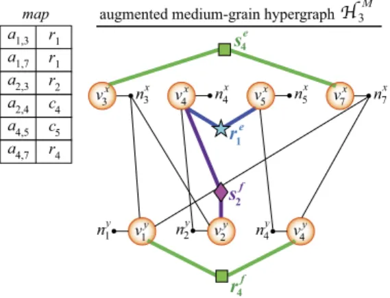
Fig. 6displays the medium-grain hypergraphHM₃

=

(V3,N₃M) augmented with message nets, which is formed during bipartition-ingA3,X3andY3given inFig. 4. The table in the figure displays

map(ai,j) value for each nonzero inA3computed by the heuristic

described in Section 2.5. Augmented medium-grain hypergraph HM₃ has four message nets. Observe that the sets of vertices con-nected by expand-send net se

4 and fold-receive net r

f

4 are the

same for the fine-grain and medium-grain hypergraphs, which are, respectively, illustrated inFigs. 5and6. Expand-receive net re

1 connects

v

x4and

v

5xsinceP3 receives

{

x4,x5

}

due to nonzeros

in

{

a2,4,a4,5

}

with map(a2,4)

=

c4and map(a4,5)

=

c5. Fold-send

net sf₂connects

v

x

4and

v

y

2sinceP3sends partial result y(3)2 due to

nonzeros in

{

a2,3,a2,4

}

with map(a2,3)

=

r2and map(a2,4)

=

c4.

Similar to Section 3, after obtaining bipartitions Π(Ak)

=

{

Ak,L

,

Ak,R

}

,Π(Xk)

= {

Xk,L

,

Xk,R

}

, andΠ(Yk)

= {

Yk,L

,

Yk,R

}

, the

labels of the parts represented by the leaf nodes are updated in such a way that the resulting (K′

₊

1)-way partitions are denoted byΠ_{K ′}+1(A)

= {

A1, . . . ,AK ′+1

}

,ΠK ′+1(X)

= {

X1, . . . ,XK ′+1

}

, and

ΠK ′(Y)

= {

Y1, . . . ,YK ′+1

}

.

4.1. Adaptation for conformal partitioning

Adapting the medium-grain model for a conformal partition on vectors x and y slightly differs from adapting the fine-grain model. Vertex setVkcontains an amalgamated vertex

v

ix/yif at least one of

the following conditions holds:

•

xi

∈

Xk, or equivalently, yi

∈

Yk.

• ∃

at,i

∈

Aks.t. map(at,i)

=

ci.

• ∃

ai,t

∈

Aks.t. map(ai,t)

=

ri.

The weight of

v

iis assigned as

w

(

v

i)

= |{

at,i

:

at,i

∈

Akand map(at,i)

=

ci

}|+

|{

ai,t

:

ai,t

∈

Akand map(ai,t)

=

ri

}|

.

Each volume/message net that connects

v

x_i or

v

y_i inHM_k now con-nects the amalgamated vertex

v

x_i/y.

5. Delayed addition and thresholding for message nets Utilization of the message nets decreases the importance at-tributed to the volume nets in the partitioning process and this may lead to a relatively high bandwidth cost compared to the

case where no message nets are utilized. The more the number of RB steps in which the message nets are utilized, the higher the total communication volume. A high bandwidth cost can especially be attributed to the bipartitionings in the early levels of the RB tree. There are only a few nodes in the early levels of the RB tree compared to the late levels and each of these nodes represents a large processor group. The messages among these large processor groups are difficult to refrain from. In terms of hypergraph par-titioning, since the message nets in the hypergraphs at the early levels of the RB tree connect more vertices and the cost of the message nets is much higher than the cost of the volume nets (tsu

≫

tw), it is very unlikely for these message nets to be uncut.

While the partitioner tries to save these nets from the cut in the early bipartitionings, it may cause high number of volume nets to be cut, which in turn are likely to introduce new messages in the late levels of the RB tree. Therefore, adding message nets in the early levels of the RB tree adversely affects the overall partition quality in multiple ways.

The RB approach provides the ability to adjust the partitioning parameters in the individual RB steps for the sake of the overall partition quality. In our model, we use this flexibility to exploit the trade-off between the bandwidth and latency costs by selectively deciding whether to add message nets in each bipartitioning. To make this decision, we use the level information of the RB steps in the RB tree. For a given L

<

log K , the addition of the message nets is delayed until the Lth level of the RB tree, i.e., the bipartitionings in level

ℓ

are performed only with the volume nets for 0

≤

ℓ <

L. Thus, the message nets are included in the bipartitionings in which they are expected to connect relatively fewer vertices.

Using a delay parameter L aims to avoid large message nets by not utilizing them in the early levels of the RB tree. However, there may still exist such nets in the late levels depending on the struc-ture of the matrix being partitioned. Another idea is to eliminate the message nets whose size is larger than a given threshold. That is, for a given threshold T

>

0, a message net n with

|

Pins(n)

|

>

T is excluded from the corresponding bipartition. This approach also enables a selective approach for send and receive message nets. In our implementation of the row–column-parallel SpMV, the receive operations are performed by non-blocking MPI functions (i.e.,

MPI_Irecv

), whereas the send operations are performed by blocking MPI functions (i.e.,

MPI_Send

). When the maximum mes-sage count or the maximum communication volume is considered to be a serious bottleneck, blocking send operations may be more limiting compared to non-blocking receive operations. Note that saving message nets from the cut tends to assign the respective communication operations to fewer processors, hence the maxi-mum message count and maximaxi-mum communication volume may increase. Hence, a smaller threshold is preferable for the send message nets while a higher threshold is preferable for the receive nets.

6. Experiments

We consider a total of five partitioning models for evaluation. Four of them are nonzero-based partitioning models: the fine-grain model (

FG

), the medium-grain model (

MG

), and the proposed models which simultaneously reduce the bandwidth and latency costs, as described in Section3 (

FG-LM

) and Section4(

MG-LM

). The last partitioning model tested is the one-dimensional model

(

1D-LM

) that simultaneously reduces the bandwidth and latency

costs [21]. Two of these five models (

FG

and

MG

) encapsulate a single communication cost metric, i.e., total volume, while three of them (

FG-LM

,

MG-LM

, and

1D-LM

) encapsulate two communication cost metrics, i.e., total volume and total message count. The par-titioning constraint of balancing part weights in all these models corresponds to balancing of the computational loads of processors.

Table 2

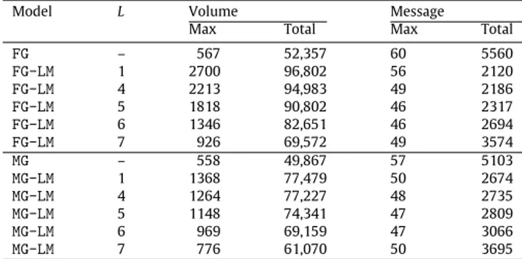
The communication cost metrics obtained by the nonzero-based partitioning mod-els with varying delay values (L).

Model L Volume Message

Max Total Max Total

FG – 567 52,357 60 5560 FG-LM 1 2700 96,802 56 2120 FG-LM 4 2213 94,983 49 2186 FG-LM 5 1818 90,802 46 2317 FG-LM 6 1346 82,651 46 2694 FG-LM 7 926 69,572 49 3574 MG – 558 49,867 57 5103 MG-LM 1 1368 77,479 50 2674 MG-LM 4 1264 77,227 48 2735 MG-LM 5 1148 74,341 47 2809 MG-LM 6 969 69,159 47 3066 MG-LM 7 776 61,070 50 3695

In the models that address latency cost with the message nets, the cost of the volume nets is set to 1 while the cost of the message nets is set to 50, i.e., it is assumed tsu

=

50tw, which is also the setting

recommended in [21].

The performance of the compared models are evaluated in terms of the partitioning cost metrics and the parallel SpMV run-time. The partitioning cost metrics include total volume, total message count, and load imbalance (these are explained in detail in following sections) and they are helpful to test the validity of the proposed models. At each RB step in all models, we used PaToH [7] in the default settings to obtain a two-way partition of the respec-tive hypergraph. An imbalance ratio of 10% is used in all models, i.e.,

ϵ =

0

.

10. We test for five different number of parts/processors, K

∈ {

64

,

128

,

256

,

512

,

1024

}

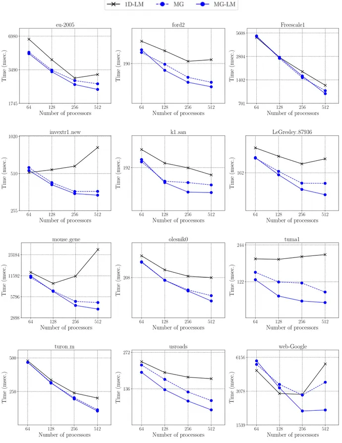
. The parallel SpMV is implemented using the PETSc toolkit [3]. PETSc contains structures and routines for parallel solution of applications modeled by partial differential equations. It supports MPI-based and hybrid parallelism, and offers a wide range of sparse linear solvers and preconditioners. The parallel SpMV realized within PETSc is run on a Blue Gene/Q system using the partitions provided by the five compared models. A node on Blue Gene/Q system consists of 16 PowerPC A2 processors with 1.6 GHz clock frequency and 16 GB memory.

The experiments are performed on an extensive dataset con-taining matrices from the SuiteSparse Matrix Collection [11]. We consider the case of conformal vector partitioning as it is more common for the applications in which SpMV is used as a kernel operation. Hence, only the square matrices are considered. We use the following criteria for the selection of test matrices: (i) the minimum and maximum number of nonzeros per processor are, respectively, set to 100 and 100,000, (ii) the matrices that have more than 50 million nonzeros are excluded, and (iii) the minimum number of rows/columns per processor is set to 50. The resulting number of matrices are 833, 730, 616, 475, and 316 for K

=

64, 128, 256, 512, and 1024 processors, respectively. The union of these sets of matrices makes up to a total of 978 matrices.

6.1. Tuning parameters for nonzero-based partitioning models There are two important issues described in Section5regarding the addition of the message nets for the nonzero-based partition-ing models. We next discuss settpartition-ing these parameters.

6.1.1. Delay parameter (L)

We investigate the effect of the delay parameter L on four dif-ferent communication cost metrics for the fine-grain and medium-grain models with the message nets. These cost metrics are max-imum volume, total volume, maxmax-imum message count, and total message count. The volume metrics are in terms of number of words communicated. We compare

FG-LM

with delay against

FG

,

Fig. 7. The effect of the delay parameter on nonzero-based partitioning models in

four different communication metrics.

as well as

MG-LM

with delay against

MG

. We only present the results for K

=

256 since the observations made for the results of different K values are similar. Note that there are log 256

=

8 bipartitioning levels in the corresponding RB tree. The tested values of the delay parameter L are 1, 4, 5, 6, and 7. Note that the message nets are added in a total of 4, 3, 2, and 1 levels for the L values of 4, 5, 6, and 7, respectively. When L

=

1, it is equivalent to adding message nets throughout the whole partitioning without any delay. Note that it is not possible to add message nets at the root level (i.e., by setting L

=

0) since there is no partition available yet to form the message nets. The results for the remaining values of L are not presented, as the tested values contain all the necessary insight for picking a value for L.Table 2presents the results obtained. The value obtained by a partitioning model for a specific cost metric is the geometric mean of the values obtained for the matrices by that partitioning model (i.e., the mean of the results for 616 matrices). We also present two plots inFig. 7to provide a visual comparison of the values presented inTable 2. The plot at the top belongs to the fine-grain models and each different cost metric is represented by a separate line in which the values are normalized with respect to those of the standard fine-grain model

FG

. Hence, a point on a line below y

=

1 indicates the variants of

FG-LM

attaining a better performance in the respective metric compared to

FG

, whereas a point in a line above indicates a worse performance. For example,

FG-LM

with L

=

7 attains 0.72 times the total message count of

FG

, which corresponds to the second point of the line marked with a filled circle. The plot at the bottom compares the medium-grain models in a similar fashion.

It can be seen fromFig. 7that, compared to

FG

,

FG-LM

attains better performance in maximum and total message count, and a