O a s & m m Ш ѣ т к Ш ш т ш т м т Ш ш М ё т т ’·♦*' , ♦·· í«r. ' V . Μ -г.·^*,. ,.,, è^s«/ ΐύ-¿3La¿ ‘.íi^' В щ 0 ш ѣ т , ,··'!*^· ,^·· ■': ■.;·, ,S< Ѵг.. V ■ if. ?;ί· "■•t* ■'‘S o /v Г-лу^ - .Д ·,:: %*'., >*· ?»:·.·;.*·>î“.· BUSin^èC'\ i l · Д . r f i '?/■ T ‘■/'.^ ‘ J ^hhShblhll jv *"<',·*^. · <«·. ·* · ;*·> «jii ·
4^ '-* -Lv>^" k e n t Uïii*^/ '·* »Sii 'Л‘ < ‘•г *** ‘i» wC:>'^ ·Β> y'7
^ ^ л''":. X hl "ïMf ^
*·>· г ·;,'-»^ ·> ί
/5 ν'.·) .г-»‘i?“-Зи^ *^»'Р .•г::·.*''?*!''♦»ί>. Ç‘.i·«> h
Coîîimorı S ' - o c k R e t u r n s a n d I n f l a t i o n : A n I n v e s t i g a t i o n o f 1 s t a r . l ) u l S e c u r i t i e s E x c h a n g e A I ' h e s i s S u b m i t t e d t o t h e D e p a r t n v e n t o f M a n a g e m e n t a n d 1 hie G r a d u a t e S c h o o l o f / B u s i n e s s Adni i n i s t r a t i c : / o : B i l k e n t U n i v e r s i t y i n P a r t i a l F u l f i l l m e n t o f t h e R e q u i r en>ent s f o r t h e D e g r e e o f M a s t e r o f B u s i n e s s A d m i n i s t r a t i o n b y R . T . K A R T A L C A G L I S e p t . , 1 9 9 0 Blîbcl.'ül·. TTjflî7at*d'h7 lUhxfoy
и &
I certify that I have read this thesis^ and in my opinion^ it is f u l l y adequate in scope and in qualify^ as a t h esis for the d e g r e e of Master of Business Administration.
Assoc. Prof. Kursat Aydogan
---I certify that ---I have read this thesis, and in my opinion, it is f u l l y adequate in scope and in quality, as a thesis for the d e g r e e of Master of Business Administration.
Assoc. F’r of. Umi t Er ol
I certify that I have read this thesis, and in my opinion, it is f u l l y adequate in scope and in quality, as a the s i s for the d e g r e e of Mast'er of Business Administration.
Assoc. Pr of . Gokliari C a p o g l u
A p p r o v e d by the G r a d u a t e School of B u s i n e s s A d m i n i s t r a t i o n
AEGTRACT
Corrizn stock RetumE and Inflation: Pr :nvfc-E>tigatiDn of Fishier Effect
for
" Irta n b L il S fr'cu ritie s Exchange
R . T . Y^PRIPL CAGLI
MBA in ManogeTieht
S u p e r v is o r : lAssoc. P r o f . K u rs a t A yd o crr
Sept., 199C), 68 pages
This study investigates the existence of a relaticriship cet^^ıc-eгı returris or. conmon stccks and expected inflation i' lurke.. Ihie relationship: is tested within the fram£?v^ork of Fishe- Effect wising a single ei.i£^tion rezression mcDdel. The regressior» pa.raniete'~E are tested tc see whether an increase in expectez inflatizn is accoTip£vnjer by an ec-ic.l increase in nominal returrs. leavi-i the real rate cznstarit. T^x? test results sho-j that, when actual inflation rates are used to proxy expected inflaticr. hypothesis of existence c* Fisher Effect on stock returns is rejected; arc that it fails to be rejected whien Box Jenkins red^esentatizr. of inflatioTi IS used as the proxy. The dichotoory is Sviderice c' t^ie fact that ihz test results for Fisher Effect c"e n)ctr-cco3ogy dependent, and thiat inferences on Fisher's Theor~y snould t>z made with cauticr..
ÖZET
Hisse Senedi Kazançları ve Enflasyon; İstanbul Menkul Kıymetler Borsası’nda
Fisher Etkisi üzerine Bir Çalıçma
R.T. KARTAL CAGLI
Yüksek Lisans Tezi: İşletme Enstitüsü Tez Yöneticisi: Doç. Dr. Kür şat AYDOöAλ
Eylül 1990, 68 sayfa
Bu çalışma Türkiye’de hisse senedi kazançları ile enflasyon beklentisi arasında bir ilişki olup olmadığını ar aş ti r maktadı r . Varsayılan ilişki, Fisher Etkisi çerçevesinde, tek cenklemli bir regresyon modeli ile test edilmiştir. Regresyon katsayılarının değerleri test edilerek, beklenen enflasyonda meydana gelen bir artışın, reel kazancı sabit tutacak şekilde, nominal kazançlarda da aynı oranda bir artışa yol açıp açmadığı araştırıI ra ştı r. Test sonuçları, modelde beklenen enflasyon yerine gerçekle5 enflasyon rakamlarının konulması durumunda hisse senedi kazançi ar ı nda Fisher Etkisi olduğu savının çürütüldüğünü; Box Jenkins Yor.*, emi ile modelienmiş değerler konulduğunda da çürütUlemediçi ni ortaya koymuştur. ^Bu ikilem, Fisher Etkisi *ni ölçmeye yönelik test sonuçlarının kullanılan yöntemlerden ne denli etkiI endiğini , ve Fisher’ın Teorisi ile ilgili çıkarımların çok dikkarle yapılması gerektiğini ortaya koymuştur.
Anahtar Kel i mel er: Fisher Etkisi, Beklenen Enflasyon, _’yar 1 anabi 1 i r Beklentiler, Nominal — reel Kazanç, Box Jenkins Yont era , Ekırağanlık
ACba\OAjL£ix3aiDNíTS
1 i-jculd like lo 1к»£лГік E>r. Kursat Aydogan for his si-tpers'isim
in dsvslopTie’it of іь»э the-s^is. 1 i^^Lild like lo t^■iaí·ïk Deparl'"»s-:"»t of Мс;пасівт>ЕГі1 of Biif.erit Lkiiversity for providirç· me with an invaluabie fE«A educeticjn. Special th¿=vnks go lo ail those pe-ocio whc« vvere? kind ecid itnderslar»ding to me duririQ de\'elDp;Tr:£Tit of tho thobis.
t a b l e o f CONTENTS: Abst r a d Ozet Ac knowl edgement s Table of Contents List of T a b l e s List of Figures 1 . I n t r o d u c t i o n A. Fi sherds T h e o r y B. Opponent Vie^ C. Intermediate V i e w
D. Relationship of Fisher Effect w i t h Common Stocks II. P r e v i o u s Theoretical and Empirical Work
III. M e t h o d o l o g y
A. A Restatement of Fisher's Model B. Modifications for OLS Estimation C. Selected Models
D. Statement of T h e Hypothesis to be Tested E. Tlie Data 1. Survey of R e t u r n Data 2. Analysis of R e t u r n Data 3. Survey of I n f l a t i o n Data F. Modelling E x p e c t e d Inflation 1. Expectations Scheme
2. Sear c h for a Legitimate Adaptive Model 3. MetJiodology to Represent Adaptive Scheme G. B o x Jenkins Analysis of Inflation D a t a
1. Stationarity Rendering 1 1 111 IV vi vi 3 4 4 6 20 2 0 21 23 23 24 25 26 27 29 30 31 32 33 33
3. Model I d e n t i i i c a t i o n 3. Model E s t i m a t i o n 4. Diagnostic Check 5. Parsimony Check
6. Discussion of the Model
H. Assumiiitions and Limitations , V
IV· R e s u l t s
A. Regression A n a l y s i s Results B· Results H y p o t h e s i s Tests
V. Conclusions
A. Fisher Effect i n T u r k i s h Stock Market
B. Implications for Stock Market Praclitioners Selected Bibliograp>hy Appiendi x 34 35 35 36 36 37 39 39 43 44 44 45 48 51
LIST OF TABLES
Table 1. Results of R e g r e s s i o n of In f l a l i o n Against T i m e for De-irending the Data
Table 2. Box Jenkins ARl x Seasonal AR E s t i m a t i o n Result s
Table 3. Regression Results, Fisher E q u a t i o n
Table A . 1. The List of Surveyed Stocks and Their Market Betas
Table A. E. The List of Five Portfolios Constructed, w i t h the lists of Stocks Included in E a c h
Table A. 3. Table of A R I M A Est i m a t i o n Results CSASJ Table A. 4. Summary S t a tistics of Theil P r o c e d u r e for
De-trended Inflation, model ARl
Table A. 5. Summary S t a t istics of AUTOREG Procedure Table A. 6. Hypothesis Test Results, for Model with Actual I n f l a t i o n as Independent Variable Table A. 7. Hypothesis Test Results, for Model with
Expected I n f l a t i o n as Independent Variable
35 40 52 52 60 63 66 67 68 33 LIST OF FIGURES
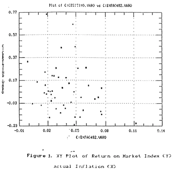
Figure 1. XY ^Plot of R e t u r n o n Market I n d e x CYJ vs Actual I n f l a t i o n CXJ
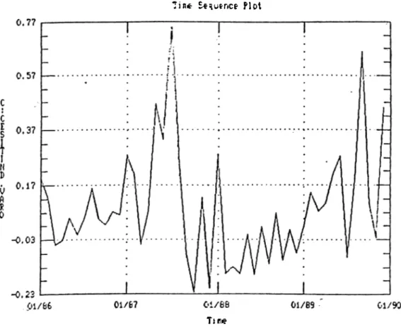
Figure A. 1. Time Plot of R e t u r n on Market I ndex
Figure A. 2. Time Plot of R e t u r n on Index a n d Inflation Figure A· 3. Time Plot of R e t u r n on Index and Inflation
with unequal scales to see co-movement
Figure A. 4. Monthly I n f l a t i o n Cpercentage chan g e in CPI !> Turkey Cl 981: 2 - 1990:1) 39 53 54 55 56
Figure A. 5. Time Plot, Residuals from R e g ression of Inflation a g a i n s t Time for De-trending
unequal scales for observing co-movement
57
Fi gure A. 6. ACF/PACF for De-tr ended Inflation Series
CSAS) 58
Figure A. 7. ACF/PACF f or Residuals (of ARIMA Model 61
Fi gur e A. 8. Time Plot of Actual and Expected I nf 1at i on 64 Fi gur e A. 9. Time Plot of Actual and Expected I ni l ati on
I. INTRODUCTION:
For over a decade, sustained inflation is one of the most important problems of Turkish Economy. Despite the efforts in recent years, its pace could not be slowed down, and it has fluctuated around 60-75 percent annually for the last few years.
During these years, the Turkish Financial System has gradually witnessed important developments. But perhaps the most interesting development was the establishment of Istanbul Securities E x c h a n g e CISED in 1986. Evidently, the stock market in Istanbul has revived great interest both for investment community, and corporations which are tired of high borrowing rates.
Despite such developments, still there is the discussion of whether severe inflationary conditions would adversely effect the development of the capital market. Especially from the point of view of the individual investor, it is a question of whether
inflation will adversely effect stock returns or not.
The objective of this thesis is to attempt in detecting adverse effect of inflation on returns of stocks traded in ISE, if any such effect exists. Formally, the study will focus on testing whether the Fisher Effect is applicable to returns of stocks traded in Istanbul.
Globally, ,an analysis of past returns over inflation rates show that stock returns have historically outperformed inflation rates. Consequently, some people build on this very long run evidence in concluding that inflation is not a concern for common stocks, and state that common stocks are a hedge against inflation.
For one thing, for a financial instrument to be a hedge against an uncertain event, like a change in the price level, the
real (inflation free) return on that security must have zero covariance with occurence of that event (the inflation rate). But when one speaks of a statistical variable being larger than another variable, he is simply making a comparison of magnitudes rather than comparison of co-movements. Therefore, observations that past rates of returns have been above inflation rates have nothing to do with the theory of whether·stock returns are a hedge against inflation.
But why should common stocks be a hedge against inflation? The rationale given by t r a d i t i o n a l economic t h e o r y is as follows:
A stock represents ownership of physical capital, of which value is assumed to be independent of the rate of inflation. Corporations earn income through their operations of real assets, while inflation is a monetary phenomena. Under competitive pressures, with inflation expected to continue, the firm's prices,
required rates of return, and for an unlevered company, costs, profits, dividends and stock prices would rise at the same rate as prices (actually, at a faster rate for a levered firm). Since corporations can deduct high nominal interest expenses, only their accounting profits decrease. Actually, firms retain their real debt. Increased debt allows both paying interest and dividends
(maintaining real dividends) and reinvestment.
However does the traditional theory hold in reality? Since, expost, real returns are the difference between nominal rates and effect of inflation, obviously, had there been lower rates of inflation with nominal returns kept fixed, real returns would be higher in the past. So one could say that it did not hold.
and hence, the relationship between expected real returns on common stocks and expected rate of inflation should be examined.
Unfortunately, the theoretical relationship between expected real returns on assets and expected inflation has its foundations in a historically controversial issue of Economics and Finance literature, THE F I S H E R EFFECT,
A. F i s h e r ’s Theory:
The discussion dates back to early 1900's. First in
" A p p r e c i a t i o n and Interest"ClS96!), and then in "The R a t e of Interest"Cl 930) (revision, "The Theory of Interest" C1965)), Irving F i s h e r suggested that:
..The rate of interest in the (relatively) depreciating standard (currency) is equal to the sum of three terms: the rate of interest in the appreciating standard (real goods), the rate of appreciation itself and the product of these two elements...'
R = r + n + rn
where for example R is the yield to maturity of a discount bond, n is the inflation rate expected to prevail over the life of the instrument, and r is the real rate of return (he did not define return terms in expectation form since keeping the security until maturity would suffice to ascertain the return from the
instrument). If individuals could foresee the inflation in the future, the market would adjust in such a way that the expected inflation rate would be added to the real rate of return (as determined by real factors of the economy) to form the nominal rate of return. Fisher stated that expected real rate of interest is independent of the expected inflation and is basically constant. He
also added that the relationship, hence, between expected nominal returns and expected inflation is not only positive but also one-to-one, thereby changes in n not effecting r.
B. O p p o n e n t view:
On the contrary, the Keynesian economists follow Robert M u n d e l l and James Tobin and suggest that under inflation, the individuals' monetary assets depreciate and hence their real wealth shrinks. This decrease in wealth, they say, increases saving behaviour and increased demand for investments in securities reduces the market rate of return ( T h e P i g o u Real W e a l t h Effect).
The defenders of P i g o u Effect also deny a constant real rate and believe that real rate fluctuates with inflationary disturbances.
C. I n t e r m e d i a t e Views:
Finally, members of a third group like M i l t o n Friedman,
suggest that the Fisher Effect holds for riskless securities only in the long run, and that in the short run, an effect similar to Pigou Effect is observable. In other words, they believe that the pcsitive effect of expected inflation shock on nominal returns is net observed instantaneously, but rather that market adjusts with a
*
lag. They claim that individuals should be taking a fairly long view as short' term gains are only a part of long term accumulation cf wealth into the future, and that they are altering their opinions very gradually.
There is indeed a fourth view, though not much appreciated, tnat the increase in nominal returns should be more than inflation ohanges so that real returns are net adversely effected due to
D. Relati o n s h i p of Fisher Eff e c t w ith c o m m o n stocks;
While the discussions for the acceptability of Fisher Effect
prevailed for money market instruments, Eugene F a m a has hypothesized that if mar.-'.ets are highly efficient, the Fisher Effect would hold for all assets including risky securities like common stocks.
In the next section, challenging problems in testing Fisher's theory are discussed.
II. PREVIOUS THEORETICAL AND EMPIRICAL WORK:
The problems■with testing Fisher Effect (or inflation return relationship) arise in three basic categories:
15 There is conflict among economists on the description of the correct type of econometric model to use in representing the relationship between expected nominal returns and expected inflation.
il5 For those models that embody expected, rather than observed, variables, there is the problem of data to use. This problem gets even complicated when some researchers tend to assume that
individuals form their expectations according some scheme, while others may adopt another.
iii5 Especially in the case for common stocks, a maturity is not defined. Hence it is difficult to fit them into the Fisher's framework.
F i s h e r C 1896,19305 himself tried to test his hypothesis on interest rates using the model:
R = r + En (since rn was negligible for US)
In preparing the data set he used yieId-to-maturities on discount
*
bonds. He stated in his writings:
'..a method of return determination between two points in time is not necessarily the "expected“ one at the first date unless the latter of two dates is the maturity..'
econometric time series was not well defined). As a proxy for real r he utilized difference between yield on bonds payable in gold, and that payable in money. He analyzed US & UK data, and found no significant correlation between interest rates and change in WPI. While he expected a correlation close to one, maximum effect that he could find was 0.4 fcr US and 0.6 for UK (with a lag of four years). He himself ecu Id not explain the phenomena well and attributed it to imperfect foresight. Nevertheless, he observed that interest rates were high when price level was high ,and low when low.
Research on inflation - return relationship was hardly studied after Fisher until '50's and '60's when inflation began to be increasing. After this time, while economists concentrated on testing and/or redefining inflation - return relationship for interest rates, researchers in finance sought for the existense of effect in common stocks.
MundellC1963) discussed inflation and real interests within the framework of Pigou Effect.
GibsonC1970) analyzed interest rates and inflation expectations using a distributed lag model of changes in inflation rates upto 10^^ lag (as a proxy for expected change in inflation ) against changes in interest rates.
10
dR = a + Z ^ dn
He found a positive relationship, though with a factor smaller than that specified by the t.heory. He attributes his findings to a "slow" market adjustment mechanism. He also takes idea of a constant real rate with suspect. He worked with incerest rates and
found positive but negligibly snail regression coefficients. Nevertheless, he remarked that the absence of measurement of Fisher's relationship seemed not to have detracted from its theoretical acceptability.
FamaC1975D tried to construct the exact form of FialMfcar's model:
where expectations are conditional on available information a period in advance. He checked whether bond market is "efficient" in Fisher s e n s e by testing the following model:
n = a + b R + £^ where the variable R represents returns of one month T-Bills. He found "b" to be 0.98. He concluded not only that bond market is efficient in Fisher sense, but also that he could safely use interest rates on T-bills as a proxy for expected inflation since historically this instrument had given returns at levels almost equal to prevailing inflation rates.
Gibbons, Fama and S a n t o n also give support to the view of constant real rate empirically.
S a n t o m e r o C l 9733 worked on theoretical structure of the inflation interest rate relationship. Santomero refused the models
*
that assume independence of inflation and real return, and suggests that a link may form between these two variables in case a change in growth rate of economy occurs. He also objected to single equation systems of modelling and claimed that the relationship should be analyzed within a general equilibrium framework.
coEmit errors in statistical inference.
TobinC1974) stated his belief that increases in n are perceived by the market as signals for Fed to slow down economic growth, which hampers stock values.
Fanva and SchwertC1977) remarked Fisher's view of real and monetary sectors of economy being largely independent. They depended on that assumption for studying the relationship without reference to a complete general equilibrium model for real returns. They said that since a regression estimates the conditional expected value of the dependent variable, an estimate of of ft coefficient in the regression,
Rt= " + ^ ^^^t ^t
which is statistically indistinguishable from 1.0 would be consistent with Fisher.(Thereby making the assumption that
individuals are quite perfect in their foresights so that expected values are equivalent to actual ones). For returns, they utilized returns of one value weighted and one equally weighted portfolio; whereas they used CPI for inflation. As a measure of expected inflation, the authors assumed that expected real return on T-bills to be constant through time and that nominal returns on T-Bills are equal to expected real return plus expected inflation.
They obtained their expected inflation series by assuming the interest rate on a T-Bill maturing at the end of period t as a proxy for expected inflation. Their analysis suggested that common stock returns are negatively related to expected inflation rate, and that only one asset, real estate, has a nominal return behaviour in one-to-one correspondence with expected and unexpected
components of the inflation.rate. They, however, also stated that the negative relationship explains only a very small portion of variation in stock returns.
B o dieC1976), discussing hedge property of common stocks, tried to find how effective a portfolio of stocks was in reducing the real return variability of a pure discount bond of holding period maturity. He observed that:
the higher the ratio of variance of the non-inflation component of real returns on common stocks, to the variance of unanticipated inflation, less effective the stocks as inflation hedge.
His result showed that real return is negatively related to both expected inflation n and unexpected inflation (n - EH). His suggestion to investors was to sell stocks short for hedging.
M a r t i n FeldsteinCl 976!) and later MilesC1983!>, V an H o r n e C 1 9 8 4 ) , TanziC1984D attracted the attention to the issue of taxes, and individually suggested that changes in returns should be higher than changes in inflation rate in order to offset abrupt effects of taxes.
N e l s o n C 1 9 7 6 ) studied relationship of stock returns and inflation. He regressed ex post nominal returns on ex post inflation and’ found negative relationship. He suggests the following rationale:
^t " ^^^t ^t-1^ "t = ^<"t ^t-1^ "t
= = > = a + + (a " + u^
-where the properties of least squares depends on value in paranthesis. He shows statistically that if Cov(£^,u^) < 0 , that
is market reacts to unexpected n, then /5 could in fact be negative. Consequently, he tries the test with lagged n's. He finds all lags and leads (including zeroth lag) negative. Nelson also modeled expected inflation in an ARMA(1,1) framework (in my opinion, his coefficients suffer from non-stationarity and non-invertibility) Two of worth-noting suggestions by Nelson are
i) ex post, it could be possible to gain higher real returns than buy and hold strategies in the market.
ii) Lintner's idea that firms' increased dependency on external financing during times of inflation could create a link between expected real returns and expected inflation is highly plausible.
In 1S79, portfolio selection dimension of stock return inflation relationship came into question. ManasterC1979D
investigated the theoretical framework and stated that real and nominal efficient sets are either identical or disjoint; and that, if they are identical, returns should depend on covariance with inflation. He also suggested that in case the sets were disjoint, no two portfolio could be both nominal and real efficient.
B r e n n e r and SarnatC19793 tested statistical similarity of distributions of real and nominal portfolio returns ex post. They also analyzed jihether investing on the basis of nominal returns had done any harm ex post in real terms. They suggested upon their analysis that, ex post, real and nominal returns showed a very similar stochastic behaviour, (probably due to small significance of inflation) ,and that it would have done no harm in following Markowitz's nominal framework in investment decisions.
Another interesting event of 1879 in literature was work of
FirthCl979D. Following the research of BodieCl976D and others, he analyzed behaviour of stock market returns against inflation in UK. Unlike other research results, this study conveyed the idea that not only the stock market returns in UK have positive correlation with inflation rate, but also that the effect is more than one-to-one.
Namely, it is observed that a change in inflation rate in UK causes a change of same sign and larger magnitude in stock carket r^urns. Given other findings in literature that are not in favor of Fisher's Theory, Firth himself had difficulty in explaining how and why this theory should hold in one part of the world while it does not in many others.
Sargent and LucasC1981D surveyed inflation - return
relationship in interest rate framework. While they object to single equation models for inflation - rate of return relationship for the latter has dependence on real production, investment, price level etc., they also deny utilizing "simple" goods market - money market equilibrium models for testing the Fisher Effect since this methodology requires vertical LM, or horizontal IS curves, or vertical Phillips curves for Fisher to hold. They suggest that joint hypothesis of natural rate of unemployment and rational
*
e x pectations is a sufficient substitute to Fisher's theory in testing inflation - interest rate relationship.
Fama C1981) worked out stock returns - inflation relationship for the post 1953 period. He searched for a proxy effect as the cause of a negative relationship between real stock returns and inflation. He hypothesized that there should exist a strong
negative relationship between inflation and real production activity in the economy within the framework of quantity demand for money. He also hypothesized that there existed a positive relationship bet-een real activity and stock returns due to the positive effect of improving real activity on the capital expenditures process. F ama expected that these two strong correlations in reverse directions could be the cause of the negative relatic.oship between stock returns and inflation observed
in the literature.
However, not only were his proxies of expected real return, future real acoivity and inflation variables prone to naive assumptions, but also he hardly faced a strong evidence in studies that confirm his rationale. Fama explained that, for many maturities, his failure to observe the relationship was due to overlapping of the two positive and negative effects.
FriedmanC1982) divides phases of market response to changes in monetary growth in terms of interest rate changes into 3:
i^Initial effect of an increase in money supply reducing nominal returnsC liquidity e f f e c t )
ii)Investment of excess cash as well as low market borrowing rates attract businessmen ( i n c o m e effect)
iii^In long terr, change .in nominal rates are equal to changes in inflation (the Fisher Effect)
The focus of G e s k e and Roll'sC19833 argument concentrated on the idea that a decrease in stock prices signal changes in government's fiscal and monetary policies leading to inflation, namely they suggested a "reversed causality". T i t m a n a n d Warga
(1987) tried to test a similar argument of whether stock returns are predictors of inflation. They, like some other researchers, faced some evidence of a causality.
By 1883, studies of Fisher Effect at the international context is observed among researchers. S o l n i k C l 9 8 3 1 worked with nine major stock markets of the world to observe inflation relationships. He used interest rates as proxy for expected inflation, and observed that the Fisher's theory about independence of real returns from inflation is not supported. He cites evidence of a seasonal pattern in inflations not reflected by interest rate proxies. He has constructed his regression equation in an expected - unexpected inflation framework and found ft coefficient negative. In fact, those of unexpected component are incredibly large.
Solnik also followed Geske and others' argument of reversed
causality and found significantly supporting results via use of an ARIMA transfer function model for generating ex ante real returns.
GultekinC1983, r e p r i n t 19861 analyzed 26 countries to see if Fisher Effect holds for the stock markets of these countries for
the post World War II period.
He quotes the following equation as Fisher's Equation: = » + > E ( n j
He worked with:
i) Contemporaneous inflation rates
ii) Inflation, decomposed as expected and unexpected (via ARIMA) iii) Short Term Interest Rates as a proxy for inflation
indistinguishable from 1) Gultekin notes that a possible explanation can be the "errors in vari a b l e s p r o b l e m ” :^ G u l t e k i n
suggests that regression of stock returns on past n's should eliminate the bias since past inflation contains r.o new information. For that purpose, he used multiple regressicr. in a distributed lag framework:
R. = o +. Z /3 n . t v=i 1 t-l
He utilized sum of beta coefficients as a t-distributed test statistic for testing Fisher Hypothesis. In his deductions, the results are not in favor of Fisher. Two parameters are observed to be no different than unity:
/?2 UK
/?э t
1.292 2.24 USA 1.000 1.49
ii) ARIMA results for П mostly ended up with first difference MAI models with close to .9 parameter estimates, while for a few countries there are seasonal components also.
R z a + ^iE(n ) + ft2 in - Е(П )3 + £
In that model, the second term on the right, the unexpected component, is the residual from ARIMA procedure. The only significant is for Norway, and /?z for UK (both are positive). Negative significants are for Spain and Switzerland;
* (52 for USA.
iii) Short Term Proxy Results:
Unsatisfied with ether methods, G u l t e k i n used 90 day T Bill rate as
For this econometric problem see BaconClQSSl or NelsonC19761
a proxy for quarterly inflation. n = ot + + c
t t-1 t
and significant for most countries. Actually, it is close to 1. Regressions of stock returns on expected and jnexpected
2
inflation is done by Seemingly Unrelated Regression Mocel(SURM) . Here, G u l t e k i n confesses that:
i) a comparison can not be made between monthly and quarterly results
ii) there may be an implicit negative relationship between change in interest rates and stock returns.
Nevertheless, the regression results were still in favor of rejecting Fisher. G u l t e k i n also tried to test Fisher Equation for cross sectional data of long-run averages over the post war period. The following figures were obtained for 1947-79 period:
last 15 years overall max Industrialized countries: ft : 0.950 1.425(:*:) 1.425
25 Countries : 0.453 0.789 1.159
(*) ft=0.75 with t=1.96
In another study, GultekinCl983l attempted to utilize ex ante Liv i n g s t o n Survey of Expect a t i o n s for inflation component in Fisher Equation, rather than an ex post term.
*
G u l t e k i n tried to utilize their "Forward" expectarions given one-period prior forecasts. Namely,
E(n^^^) is specified by participants E(rit^2) is also specified by participants.
these term structure basée expectations into the future ^'■^t+2^ can be used.
Gulte k i n averaged these forecasts over each forecaster and performed the following regression:
E(R^)' = « + ^E(n^)
-and found out that ft >> 0 or 1. He suggested that it may be due to a relationship between real returns and expected inflation, and ot may be variable.
He allowed a time varying real rate using dummy variables while keeping ft as constant. As a result, he found ft as exactly indistinguishable from unity. Gulte k i n concluded that the negative reaction to inflation in contemporaneous regression nay actually be directed towards unexpected component.
To re phrase, following are the conclusions of Gultekin:
i) Ex ante findings are remarkably different than ex post
ii) There is a positive cne-to-one relationship between nominal expected returns and expected inflation
iii) Expected real return is not constant overtime iv) Expected real return is positively related to E(n) v) Results are not in faver of Mundell's Pigou Effect.
S a r a c o g l u C 1 9 8 5 1, in his study of the relationship between
*
expected inflation and interest rates for biggest five industrialized countries, utilized a VAR(Vector Autoregressive) methodology of system of equations. He used annual rates of change of money stock, monetary base, industrial production. CPI and short term interest rates. His findings suggest that real rates are not constant over time but highly variable and autocorrelated. He has
observed a non-zero correlation between real rates and expected inflation.
F r i e n d C 1 9 8 6 Danalyzed the effect of inflation on corporate profitability and stock valuation. He cites a survey result of NYSE where respondents replied that they would keep more of their balances in stocks, had there been lower inflation (but in my opinion, this increased demand for stocks ,if any,would decrease real returns in the market, assuming limited supply) F r iend
examplifies uncertainity about retained earnings and working capital needs as possible rationale for negative reactioni, to inflation. In his comments to observed positive relationships of stocks to inflation in England and Israel, he notes that depreciation policies of these two countries are more liberal than others'. He also notes that if an ex ante measure of uncertainity could be incorporated in the models, the negative observed relationship would dissappear from the results.
SksydemirCl9893 utilized Faina’s approach of modelling expected inflation for Turkey. He made use of interest rates on 1-mcnth time deposits as a proxy for expected inflation of a month ahead. Unfortunately, the sampling period corresponds to a time when interest rates were either fixed or pegged. Moreover, the stock returns cover also the period prior to establishment of stock exchange in Istanbul, and return data may be deficient due to infrequent trading (in fact these returns constitute half of his sample). He worked with nominal stock returns against expected inflation, and found coefficient of expected inflation not significantly different from zero. Then he regressed real returns
(derived by subtracting inflation from nominal returns. against
3
expected i№^*J«tion.
In any case, Soydemir reports that he has found a negative relationship between real returns and expected inflation, but admitts that his coefficients are still not significant.
I suspect that by subtracting n from R to obtain r, he may be creating an artificial negative correlation between r and n, if his expected inflation series has high correlation with actual inflation series, i.e.
and, = "t - "t
= a + f3 En^ and if 1 - Corr(n^,Er._) = e where e is small)
III. M E T H O D O L O G Y :
A. A Rest,at.ernent of F i s h e r ' s Model:
Fisher's model states that expected nominal return represents sum of E(r), E(n) and Z;r).E(n), where E is the expectations operator, r is the real return and n is the inflation rate. More formally,the model is
E(R^) = E(r^) + E(n^) + E(r^).E(n^)
where R is the nominal return. The last term on the right has always been ignored by many researchers, but given 60-70% annual inflation rates in Turkey., it would be unwise to ignore this product term, and therefore this product term is retained in the model for this study.
Unfortunately, the model contains three unobservable variables (expected variables). Therefore, a way must be found to proxy at least some of the unobservable variables. Here a simple rule-of-thumb will help to decide which variables to proxy. Since' ex post, nominal returns and inflation rates are readily observable, attempts to design proxies for their expectations is more sound than following this process for real returns which ,expost, are the difference of the former variables, nominal returns and inflation.
*
As some researchers in literature as well as Fisher himself did, an assumption will be made here that long run average expected
4
real return on a security should have a constant mean, but that return should vary around that mean with a disturbance term
Once real return is assumed to be a constant, then .oomes the issue of expected nominal returns and expected inflation.
The common methodology in the literature is to assjme that expost nominal returns are conditional expected values , where individuals in the market are believed to predict, :n the average,
5
the actual returns (which is nothing but a rational expectations assumption with close tc perfect foresight). While this assumption is also open to discussion, the methodology in the literature will be retained in this study also and actualized nominal returns will
0
be used instead of their expectations.
As for expected inflation, there are numerous methods of modelling, and the possible branching starts from the root - the expectations mechanisms. The two most popular mechanisms are rational expectations and adaptive expectations. Obviously, the researchers may never know what the individuals' actual expectation mechanism is; they can only assume one and test their assumption.
Here in this study, two alternative specifications for inflation are utilized. In the former, expectations are assumed close to perfect foresight and hence effect of observed inflation in a certain period, against return of the same period are analyzed In the latter, attempts are made to model expected inflation by utilizing some,adaptive scheme basically.
B. M o d i f ications for O L S Estimation:
Consequently, tvro alternative linear models appear in this study;
5
6
See Fama(1977)
Refer to "Assumptions and .. for a discussion of this assumption
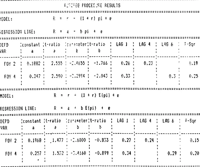
i) = r + + r . n li) = r + E(n^) +
The intention is to econometrically estimate the two models using OLS. Unfortunately, both of these two models contain specification error econoce.tr ically. For both of the models , if the structure is· represented like:
Yi = a + bl.Xl + b2.X2 where Yi :
a : r (constant)
bi ; regression coefficients
XI ; n or E(n) and X2 : r . n or r.E(n)
then there appears that variable XI is a linea r combination of X2 or vice-'versa, which is not allowed for OLS estimations'^ to be unbiased and efficient.
In that case there are two possible ways of re-specifying the models:
i) by adding 1 to left and right hand side of the equations 1 + R = (1 + r).(l + n)
1 + R = (1 + r).(l + EH) which can be log-linearized by
log(l+R) = log(l+r) + log(ii-n)
P
log(l+R) = log(l+r) + log(l+En)
In this case, an OLS regression can be performed for log(l+R) against log(l-^n) where the intercept will be log of 1 plus r.
like Y = « - X
But the regression paramet-er estimated will then be the power of (1+n) factor in Fisher's model and will represent a non-linear parameter for the Fisher's model. For example, the model solution may give a.confidence interval for /3 but the distribution of the test statistic to see the additive effect of inflation on nominal returns is hard to derive if not impossible.
Consequently, this approach is abandoned due to its uninformative nature for hypothesis testing.
ii) The second approach is a linear equation with a restriction. Namely, the specification is:
r r + (l+r).n^
by which the linear model is reduced to one explanatory variable with the restriction that coefficient of n is assumed to be 1 plus the intercept term, r.
C. S e l e c t e d Models:
To sum up, two alternative econometric models are analyzed in this study:
a) a + /3.n, +
b) "t = a 4- i3.E(n^) +
In both- cases, the models will be tested for whether
ft = 1 + a or ft - <X = 1
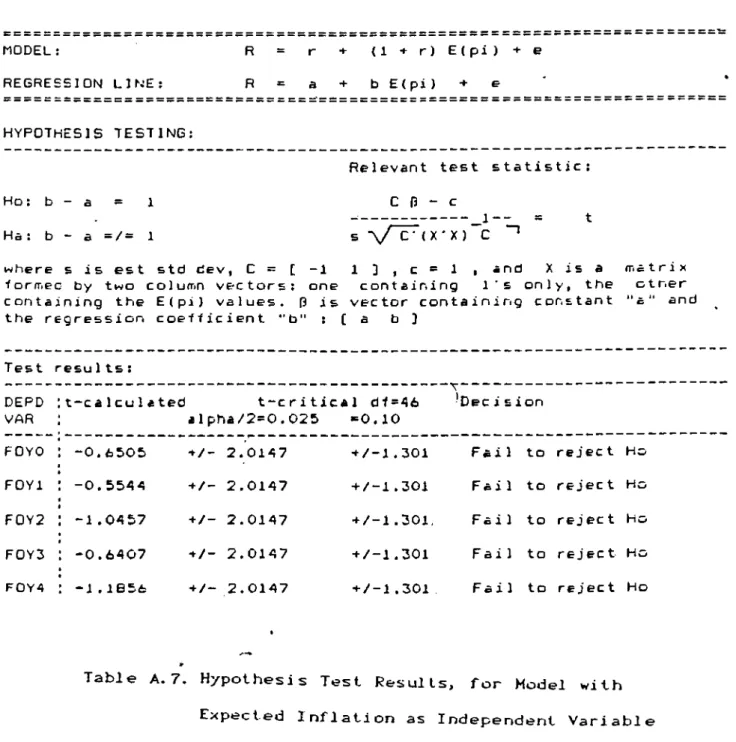
D. St a t e m e n t of The H y p othesis To be Te sted;
Formally, for both of the mode]Ls , the hypothesis to be will be :
Ho : - oi = 1 Ha : Cl - a = / = 1
The test statistic that will be utilized here is, Cb - c
'T-2 c/ -/C ' (X'X)
where Cb - c is the linear restriction ft - a. - i C = r - l l l b = | o ( T c = l
O' is the estimated standard deviation, and X is the matrix of independent variables, including the intercept.
E. The Data:
Since the two specified models differ only by the issue of whether inflation is expected or actual, a total of three series of variables are required to test the two specified models; namely R
(nominal stock returns), n (actual inflation), and En (expected inflation).
For results to be unbiased and efficient, the degrees of freedom should be as large as possible. However, as far as these two models are concerned, there is a restriction of data availability for both nominal returns and inflation.
Although even daily stock prices and hence returns are available, the shortest period of time for which an inflation figure is announced is a month. Consequently, monthly observations are used for the models.
The shertcor.: i of at the time the analysis few months more tr.ar fou: in ISE. Then, only T.e f period with forty-rirht
1. Survey of Return Data;
The stocks :r=ied The concern for degrees those stocks that :.r.ve p; filter rule reduce: 'he
For return ;alcu; utilized. In Turkey the portion of income from s: capital gains. Moreiver, return measurements is n ; to attain percentage cha: splits and stc:o d; variable.^ ^
Here, instea; of : index (base set t: 100 a: for each stock:
^ F - 1^
nis adopted sampling freque::cy : :· that, :as being performed, it hao only been a
years since the start of active trading r year period is taken as the .templing S) montlily return observât : ens .
. the first market of ISE are freedom urged for utilizi.-.g r- . ce data for each of the 48 moiv
St to 27 stock.s .
;tions, moiithly buJletins of :ividend payments represent a fai:
cks - the significant portion 'or purposes of this study. prêt:
a fundamental issue. It si.mply "es in prices (with the effect t
idends considered) as the
a -.a lyzed . t _ rns of :s . This --.,10 . : r. are y small 5 from ion of u f f i c e s s 10c k return
cted prices themselves, montr. .y price the beginning of each monte. is -tilized
100 100
where I ^ is 1 1 e in :: e
But for pur::crs cf illustration, instead te.vt:ng the.
.“ f u 11 lis t i s. p r o V : :
IMEB Ayl Borsa îti:
: İr. .able A.]., appendix, page
:ler i r u ] teni - I SE Monthly Bull· : o- 80 )
Fisher Effect for each month and every stock in the list, five portfolios are considered to be utilized in testing the Fisher Effect. The portfolios are designed such that each one represents a nearly distinct systematic risk class. This approach is realized by grouping the stocks according to their market betas.
Out of 27 stocks, an equally weighted market portfolio is constructed. For each stock in the list, a beta figure is found by regressing returns of that stock against returns of the market pcrtfolic, in a market model;
R = a + ^ R
t m
Five portfolios are constructed, where each portfolio
12
consists of stocks that have similar computed beta figures .
2. Analysis of R e t u r n Data:
The stocks in the list of 27 show a large degree of long run 13
volatility . While the returns performed a lifetime high peak during summer of 1987, they perform a persistently negative behavior starting from last months of 1987 to almost end of 1988. It is also observed that returns have followed an upward movement during the year of 1989. Apparently, the return series are generally seasonally autocorrelated.
Moreover, nominal returns have usually been much greater than
’ 14
inflation rates of same periods , except for the decline period post
12
13
14
Table A.2.,the list of stocks in each portfolio is on page 52 A time plot of'return on market index is in Fig A.I., page 53
Refer to page ,54, Fig A.2,,time plot of return on index and inflation, and page 55, Fig A.3. for a plot with unequal scales to
'87. Expost, real returns do not seem to have differed much than nominal returns due to low variability of inflation in the observed period
3. Survey of Inflation Data:
In Turkey, various general price indeces are available. Among these, three of the major sources are State Institute of Statistics (DIE), Undersecretary of Treasury and Foreign Trade (HDTM), and Istanbul Chamber of Commerce (ITO). At the time the study was being prepared, WPI (Wholesale Price Index) for Turkey were available from three of them. On the contrary, a CPI (Consumer Price Index) series for Turkey was available from DIE only. Other two had Ankara and Istanbul CPI or Cost of Living Indeces.
The base years of HDTM indeces were in 1960's, and since they are no longer compiled, whether they are suitable indicators is questionable. Indeces of DIE and ITO are more up-to-date, but price indeces of DIE have greater geographic coverage, unlike those of ITO. Consequently, DIE is found to be a preferable source.
As for selection between WPI and CPI, the rationale of informative power of index is utilized: if it can be assumed that purpose of investment is eventual consumption (as I. Fisher assumed), the use of an inflation rate for consumption goods (CPI)
»
is appropriate.
Once the decision is made to utilize CPI, the next step is to select the sampling period and frequency of CPI data for modelling expected inflation.
15
An observation also made by SarnatC197.95 for US data
The data group for CPI with largest frequency is monthly
16
CPI (non-annualized ). It is an index, for which base value 100 had been assigned to average inflation figures of 1978 - 79. The index is published since 1982 and data pertinent to 1981 are derived
17
figures (aaiong the footnotes to the published data source, it was not indicated whether the derivation had been performed by DIE or by Central Bank of Republic of Turkey). During this process, inflation figures of 11 cities had been interpolated by using DIE Ankara CPI, Istanbul CPI (1968=100).
It is also fortunate that series is post - 1980, since it may be suggested that there has been a considerable structural change
in the Turkish Economy since early eighties.
The above mentioned series up to 87:12 is taken from statistical bulletins of Central Bank of Republic of Turkey, and the rest is taken from "Rehber" (Weekly supplement of "Ekonomik Bulten") which regularly publishes DIE-CPI(monthly). The whole data starts in 81:1 and ends in 90:1 (109 obsv.)
However, what is relevant for Fisher Equation is not level but percentage change in price levels. Namely,
CPI. - CPI._.|
= ---^ X 100 CPI
t-1
Therefore the first observation is lost and 108 monthly inflation figures are obtained.
The statistical properties of inflation data is analyzed in
16
17
Türkiye Tüketici Fiyatlar Endeksi (T6) / Consumer Price Index, DIE istatistik ve Değerlendirme Bülteni / Monthly Statistical and
depth under the heading "Modelling Expected Inflation" and it is left aside until then.
Once the first two sets of variables are made available, the next issue comes to creating a series of Expected Inflation rates for the period.
F. Modelling Expected Inflation:
Host empirical work in the literature for testing Fisher Effect had attempted to use contemporaneous inflation rates expost instead of trying to proxy expected inflation. But this approach, leads to the implicit assumption of rational expectations, as well as perfect foresight on individuals' side. These attempts resulted in no significant relationship between nominal returns and inflation.
Fama and Schwert(and later Gultekin) tried using one period lagged 90-day-Treas.Bill rates as a proxy for expected inflation, and ended up with the same results as in the regressions with contemporaneous inflation. In this study, it is not possible to follow this modelling strategy, since it is very recent that interest rates on Treasury Bills in Turkey are market determined through open market operations. It is possible that other researchers caij try that in the future with more data available.
In this study, an expectation scheme common in economics literature, namely adaptive expectations for inflation is assured; and an attempt is made to model expected inflation in Turkey according to this expectation scheme. The focus of the study is on the use of Box Jenkins Time Series Models as a proxy for individuals' adaptive inflation expectations.
1. E x p e c t a t i o n s Scheme:
When the exact stoch?:- ,ic process generating the expected inflations (or the actual i.n::'lations) is not well known, the only empirical way is to make a£; imptions regarding the mechanism that creates expected inflation.
The first step in expc stations modelling comes with the issue of assuming the scheme wit i which the individuals form their expectations. There are twc' )opular expectations mechanisms in the literature: one is rational expectations and the other one is the adaptive expectations.
The adaptive expectat :·ens assumption in the case of inflation refers to the idea that exptstations are a function of past rates of observed inflation . The difficulty with this assumption is the inability to make clear whe.‘'ler market response is to the expected inflation for the future or the rates of inflation that prevailed in the past.
The rational expectations view is more general, arguing that, for the determinants of expo cted inflation, there can be no formula that is independent of tiu actual behavior of inflation. The rational expectations assi option is that people base their expectations oT inflation on all the information economically available about the future i ehavior of inflation. It implies that people do not make syst matic mistakes in forming their
. .. 18 expectations
Since technically eaking, the proponents of rational SSS&BSSSBSSSSBSSSESBSSCBB
expectations follow the idea that the market utilizes all the available set of information to form its unbiased and efficient expectations, the assumption of rational expectations ends up, in most cases, in utilizing many series of economic variables as well as their lags in a general equilibrium context , and it becomes inevitable to make use of a VAR methodology empirically.
In order not to complicate matters, in this study, it is assumed that individuals in the market form their expectations of inflation in an adaptive scheme. In fact, the observation that actual inflation series is serially correlated can be given as some evidence for that adaptive behavior.
2. Sea r c h For a L e g i t i m a t e Adaptive Model:
For an economic variable, like inflation, there can be a few possibilities of behavior. Some of them are;
i) n can be non-stochastic and its value may be known at time t-1 t
(obviously this case does not fit in)
ii) The value of is determined by some mechanism other than individuals' behavior themselves, but is a rational predictor of
from that market. Thus n^- n^is pure white noise.
iii) The value of is generated according to the scheme
and hence.
Although the third one does not have a sound basis in economic or social theory, it is a common assumption in empirical work, and its common use is attributed to the fact that it seems to
be succesful in making short run predictions . This third type of model is a univariate adaptive expectations model.
Clearly, a univariate methodology may have theoretic deficiencies in the sense that it does not incorporate interacting variables into its analysis. However, its strength lies in making short term predictions which fits into the purpose of this study more. The purpose of the analysis here is to make simple short term forecasts a period ahead, given past values of inflation, as a proxy for individuals' expectations formation.
Final importance of this methodology is that it is a univariate analysis and assumes no theory as pertains to behaviour of inflation. This is useful because, indeed, researchers do not know the information set available to individuals and they do not know how individuals process what is available to them.
3. M e t h o d o l o g y to R epresent a n Adaptive Scheme:
Although there are various econometric forecasting techniques like simple exponential smoothing etc. that assume an adaptive expectation mechanism, an adaptive expectations scheme is best represented by a univariate ARIMA ( Box Jenkins) methodology.
20
Box-Jenkins is the best methodology because, unlike other adaptive forecasting techniques, it is not automatic and rests on the judgements of the researcher in terms of the model while eliminating the need for assuming parameters, once a model form is selected. The focus of this study will be on use of Box-Jenkins
19
19 2 0
Tirie Series models as a proxy for individuals' adaptive expectations.
So if the individuals are forming their expectations of inflation in an adaptive mode; and if Box Jenkins analysis can suocesfully ,simulate that behavior, then one period ahead forecasts derived from Box Jenkins analysis can be used in Fisher's model to substitute E(n). This is the assumption made here and Box Jenkins method is used to model expected inflation in the next chapter.
G. Box Jenkins Analysis of Inflation Data: 1. S t a t i o n a r i t y Rendering:
21
The inflation rates are plotted against time . The overall behaviour seemed like a time trend (at this point, it is impossible to know whether it is a trend or a drift; or if it is a trend, whether it is linear or not).
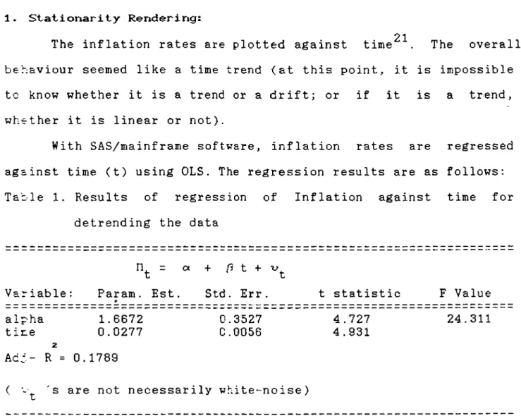
With SAS/mainframe software, inflation rates are regressed against time (t) using OLS. The regression results are as follows: Table 1. Results of regression of Inflation against time for
detrending the data
^t " Variable: Param. Est.
*
+ /5 t +
Std. Err. t statistic F Value
alpha 1.6672 0.3527 4.727 24.311
tir.e 0.0277 0.0056 4.931
2
Ac:- R = 0.1789
( 's are not necessarily white-noise)
21
See page 56, Fig A.4. in appendix
The residuals of this regression are retained fcr Box - Jenkins Time Series Analysis. The afore mentioned de-trending operation is useful in the sense that, for a Box-Jenkins methodology to be performed, it is essential that the data series be mean-variance stationary. Inflation data did not have this property prior to dertrending, and now, it is at least mean stationary.
It is a general rule to utilize differencing for transforming a non-stationary data series to a stationary one. However, this operation not only increases the variance of the series, but also may create an artificial iand usually not-invertable) MAI process. Moreover, differencing leads analyst to a rate of change concept which eventually should give results similar to those that can be obtained from a de-trended series (if the series had a trend in fact).
2 2
2. Model Identification:
The de-trended series is analyzed for autocorrelation via 2"^
visual inspection of autocorrelation function (ACF) " and partial autocorrelation function (?ACF) value plots for first 40 lags. ACF showed a positive decay pattern in first few lags and some seasonality around 6*·^ lag. PACF showed a significant positive value at lag 1 and others at lag 6 and 7. The Q-statistic
22
23
A time plot of residuals from de-trending of inflation is in Fig A.5. on page 57
(Ljung-Box) was 87 up to lag 36 with a probability of zero that the series is uncorrelated.
3. Model Estimation;
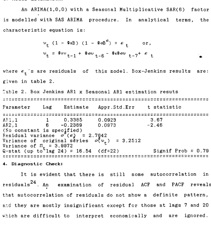
An ARIMA(1,0,0) with a Seasonal Multiplicative SAR(6) factor is modelled with SAS ARIMA procedure. In analytical terms, the characteristic equation is:
( 1 - $ i B ) ( 1 - $<sB ) = ^ or,
t u 1 t D t c t
where s residuals of this model. Box-Jenkins results are: given in table 2.
Table 2. Box Jenkins ARl x Seasonal ARl estimation resuts Parameter Lag Estimate Appr.Std.Err t statistic
ARl, 1 1 0.3385 0.0923 3.67
AR2,1 6 -0.2389 0.0973 -2.46
(No constant is specified) Residual variance ct = 2 Variance of original series Variance of n = 3.9972
Q-stat (up to^lag 24) = 16.54
.7642
= 3.2512
(df=22) Signif Prob = 0.79 4 . D i a g n o s t i c Check:
It is evident that there is still some autocorrelation in 24
residuals . An examination of residual ACF and PACF reveals
*
that autocorrelation of residuals do not show a definite pattern, ar.d they are mostly insignificant except for those at lags 7 and 20 which are difficult to interpret economically and are ignored.
24
A re-print of ARIMA estimates. Table A.3., as well as residual
ACr/PACF by SAS ,Fig A.7.,are provided on page 60, 61 respectively
Hence, model is found to be adequate.
5. P arsimony Check:
However, to see whether it is parsİEonous, it is checked whether de-trending has a significant contribution. Raw inflation series was analyzed by the same ARIMA model ARIMA(1,0,0)(6,0,0)
■ "t = t-e ' t-7 + t
Again the coefficients and $<3 as well as overall model -are found significant. But residual autocorrelations are inferior to detrended version and explained variance is 20% whereas it is around 30% in the de-trended case.
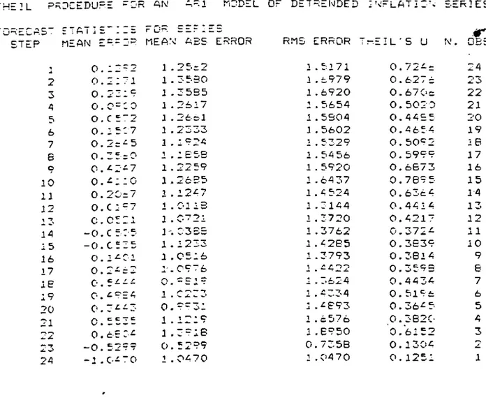
Since a Theil's U procedure could not be found in SAS and a 6-month seasonality is not available for modelling in RATS, only ARl model (de-trended) is compared to Theil's U Statistic in RATS.
25
For 24 period runs , average U statistic is 0.483 with <y = 0.17 which indicates that at least ARl is far better than naive approach.
6. D i s cussion of the Model:
There may arise some criticism to the trend parameter because it economically indicates that monthly inflation is increasing into
*
the future; however, the following rationale can be given for this approach. The analysis is univariate time series and the actual stochastic process of inflation is not known. Even if the actual process is a non-linear or very long term cyclical, it can be
25
suggested that a trend line can parsimonously approximate the behaviour cf this process during the period from '81 to '90. Moreover, the aim of this analysis is to perform back-forecasts for
inflation as a proxy for individuals' inflation expectations (given the assumption that they form their expectations in an adaptive framework). Finally, 6-month seasonal behaviour may be attributed to the fact that a good portion of workers' compensations are adjusted for inflation twice a year (6-months apart) both in public and private sectors.
Henceforth, the backward predictions of combined trend and ARIMA model for the period 86:1 - 89:12 will be used as expected
26 ‘
inflation series
H. Assumptions and Limitationst
In this study, it is assumed that:
Monetary and real parts of the economy are largely independent, which enables use of a single equation model instead of a general equilibrium model (this assumption is fairly critical in the sense that it corresponds to the assumption that monetary disturbances do not effect goods market equilibrium) This assumption is denied by many researchers in the literature.
iil> The market is "efficient" in Fama's sense so that Fisher's Theory can be extended to risky assets.
iii) Since the theoretical maturity for stocks is infinity, it is assumed that Fisher's concern for keeping the security until
26
See Fig A.8. and A .9.(un-equal scales for observing co-movement), page 64, 65 for plots of expected vs actual inflation