Default risk analysis Estimating default probability by applying contingent claims approach

DEFAULT RISK ANALYSIS:

ESTIMATING DEFAULT PROBABILITY BY APPLYING CONTINGENT CLAIMS APPROACH

ONUR VAROL

Istanbul Bilgi University Institute of Social Sciences

Master of Science Program in International Finance

Supervisor: Prof. Dr. ORAL ERDOĞAN

DEFAULT RISK ANALYSIS:

ESTIMATING DEFAULT PROBABILITY BY APPLYING CONTINGENT CLAIMS APPROACH

(FİNANSAL BAŞARISIZLIK RİSKİNİN ANALİZİ:

ORTAKLIK HAKKI YAKLAŞIMI İLE FİNANSAL BAŞARISIZLIK OLASILIĞININ TAHMİNİ)

ONUR VAROL (19402390794)

Examining Committee Members

Prof. Dr. ORAL ERDOĞAN : ... Assoc. Prof. Dr. DOĞAN CANSIZLAR : ... Dr. KENAN TATA : ...

Anahtar Kelimeler: Keywords:

1) Finansal Başarısızlık Riski 1) Default Risk

2) Kredi Riski 2) Credit Risk

3) Black Scholes 3) Black Scholes

4) Opsiyon Fiyatlaması 4) Option Pricing

DEFAULT RISK ANALYSIS:

ESTIMATING DEFAULT PROBABILITY BY APPLYING CONTINGENT CLAIMS APPROACH

ONUR VAROL

Supervisor: Prof. Dr. ORAL ERDOĞAN

March 2010, 53 pages

ABSTRACT

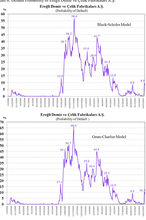
A firm’s ability to service its debts and obligations is affected by an uncertainty caused by default risk. It is very hard to distinguish explicitly among firms that would default and those that would not, before default. The only way is to make probabilistic evaluations of the possibility of default. In this thesis, the basic ideas and structures of the Contingent Claims Approach (CCA) are presented in the framework of Merton’s model that a firm defaults if its assets are below its outstanding debt. To examine the default probability (DP) of the company and to find out some implications among the parameters that effect DP, a well known iron and steel company, Ereğli Demir ve Çelik Fabrikaları A.Ş. is used. Results of the CCA approach confirms that default probability (DP) of the firm raised simultaneously together with the unattractive 2008 crisis conditions of the financial markets.

FİNANSAL BAŞARISIZLIK RİSKİNİN ANALİZİ:

ORTAKLIK HAKKI YAKLAŞIMI İLE FİNANSAL BAŞARISIZLIK OLASILIĞININ TAHMİNİ

ONUR VAROL

Tez Danışmanı: Prof. Dr. ORAL ERDOĞAN

Mart 2010, 53 sayfa

ÖZET

Şirketlerin borçlarını ve finansal yükümlülüklerini yerine getirme yetenekleri, finansal başarısızlık riskinden kaynaklanan belirsizlikten etkilenmektedir. Finansal başarısızlık gerçekleşmeden önce, şirketleri finansal açıdan başarılı yada başarısız olarak ayırmak oldukça güçtür. Tek yol, başarısızlık durumu hakkında olasılık değerlendirmeleri yapmaktır.

Ortaklık Hakkı Yaklaşımı’nın temel düşünceleri ve yapısı; Merton’un, şirket değerinin borçların altına düşmesi durumunda finansal başarısızlığın oluşacağı kabülü çerçevesinde sunulmuştur. Finansal başarısızlık olasılığını gözden geçirmek ve olasılığı etkileyen değişkenler arasında birtakım çıkarımlarda bulunmak için, demir-çelik endüstrisin bilinen şirketi Ereğli Demir ve Çelik Fabrikaları A.Ş. kullanılmıştır. Ortaklık Hakkı Yaklaşımı’nın sonuçları, finasal başarısızlık olasılığın, 2008 yılında finansal piyasalardaki kriz koşulları ile birlikte eş zamanlı olarak yükseldiğini doğrulamaktadır.

List of Figures

Figure 1: Default Interpretation in the Classical Merton Approach………...10

Figure 2: Market Value and Financial Liabilities Ereğli Demir ve Çelik Fabrikaları A.Ş……….29

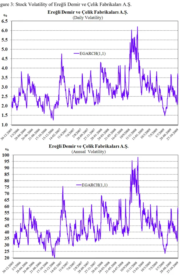
Figure 3: Stock Volatility of Ereğli Demir ve Çelik Fabrikaları A.Ş……….34

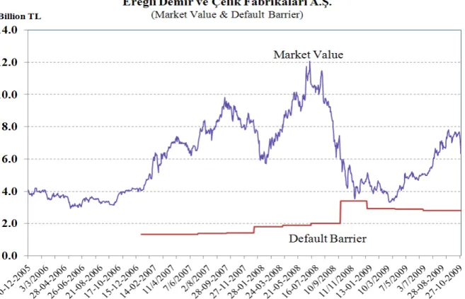
Figure 4: Market Value and Default Barrier of Ereğli Demir ve Çelik Fabrikaları A.Ş…………35

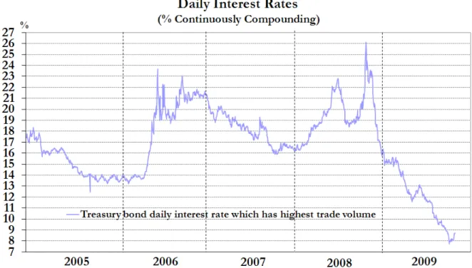
Figure 5: Daily Interest Rates……….36

Figure 6: Default Probability of Ereğli Demir ve Çelik Fabrikaları A.Ş………37

List of Tables 1- Correlogram of Stock Retuns………...48

2- AR(1) Estimation Output……….49

3- Correlogram of Residual Squared………49

4- EGARCH (1,1) Estimation Output………..50

5- Residual Tests of EGARCH(1,1) Model………51

OUTLINE ABSTRACT ... iii ÖZET ... iv List of Figures ... v List of Tables ... v I. INTRODUCTION ... 1

II. CREDIT RISK MODELS ... 2

II.1 Traditional Models ... 3

II.2 Reduced Form Models ... 6

II.3 Structural Models (Contingent Claims Approach) ... 6

III. CONTINGENT CLAIMS ANALYSIS ... 9

III.1 Theoretical Framework ... 9

III.2 The Borrower's Payoff from Loans ... 100

III.3 The Debtholder's Payoff from Loans ... 11

III.4 Option Pricing Models ... 12

III.4.1 Black -Scholes Model ... 12

III.4.1.1 Distribution of Stock Prices ... 13

III.4.1.2 Binomial Tree, Risk Neutral Valuation and No Arbitrage Argument ... 14

III.4.1.3 A Derivation of Black & Scholes Formula ... 17

III.4.1.4 Understanding

N

( )

d

₁ and

N

( )

d

₂ ... 21

III.4.2 The Gram-Charlier Model ... 24

III.5 Option Pricing Models and Probability of Default ... 26

III.6 Applying the Option Valuation Models to the Calculation of Default Risk ... 28

IV. TESTING THE MODEL AND ESTIMATION OF PARAMETERS ... 31

IV.1 The Volatility of the Equity ... 31

IV.1.2 Estimating EGARCH Model: ... 32

IV.2 The Market Value of the Equity & Default Barrier ... 35

IV.3 Risk-free Interest Rate ... 35

IV.4 Time ... 36

IV.5 Default Probability ... 36

IV.6 Duration of the Liabilities & Default Probability ... 38

V. CONCLUSION ... 42

REFERENCES ... 44

I. INTRODUCTION

The first step for evaluating the credit exposure and potential losses faced by an investor or financial institutions is estimating default probabilities for individual obligors. The fundamental inputs for risk management are default probabilities.

The contingent claims approach (CCA) was developed from modern finance theory and has been widely applied by financial market participants to measure the default probability of a firm based on the market prices of the firm’s debt and equity. In this thesis the contingent claims approach is applied to estimate the default probability of a Turkish manufacturing firm.

Unlike analysis based only on a review of past financial statements, market prices represent the collective views and forecasts of many investors, the contingent claims methodology is forward looking and helps increase the predictive power of the estimates of default risk. Given the speed with which economic conditions alter relative to the time span among releases of consolidated accounting balance-sheet information, the capability to translate continuously adjusting financial market price information into current market value estimates of asset value is especially important. In contrast, usually 90 days after the end of the quarter or annual period, accounting-based models to assessing corporate credit risk rely on historical balance sheet information which arrives with a important lag. Moreover, CCA takes into account the volatility of assets when estimating default risk. The volatility of assets is crucial in this process, since firms may have similar levels of equity and debt, but very different probabilities of default if underlying asset volatility differs.

The thesis is structured as follows. Section II reviews credit risk models which can be grouped in three categories: Traditional, Reduced Form and Structural. Section III defines the theoretical framework of the contingent claims approach and introduces technical steps of measuring probability of default. Section IV presents description of the data and results of the model. Section V concludes. Coefficients, residual tests, correlograms of the estimated mean and variance equations are provided in the appendix.

II. CREDIT RISK MODELS

Credit risk refers to the risk due to unforeseen changes in the credit quality of a counterparty or issuer and its quantification is one of the major frontiers in modern finance. The lending decision, the firm’s cost of capital, the credit spread, the prices and hedge ratios of credit derivatives, since it is uncertain whether the firm will be able to fulfill its obligation, are influenced by the creditworthiness of a potential borrower. In other words, financial decisions of the corporate institutions are affected primarily by the firms’ own risk level.

Credit risk measurement depends on the likelihood of default of a firm to meet its a required or contractual obligation and on what will be lost if default occurs. Because models of credit risk measurement have focused on the estimation of the default probability of firms, it is the dominant source of uncertainty in the lending decision.

Credit risk models can be classified into three broad categories. The first category, the set of traditional models adopt the fundamental analysis. The principle purpose of these models is to find out which factors are important in assessing the credit risk of a firm by using the potential information of financial statements to make decision about the firm’s profitability and financial difficulties. Beaver (1966) used the financial ratios of the companies to test the ability of accounting data to meet the payment of loans. Beaver (1968) expanded his study to evaluate whether market prices were affected before failure. The conclusion shows that investors recognize the default risk and change their positions one year before default. Altman (1968) tried to assess the analytical quality of ratio analysis by using the linear combination of ratios with discriminant function. In the study, the discriminant function with ratios was called as Z-Score model. Altman concluded that with the Z Score model that was built with matched sample data, 95 % of the data was correctly predicted.

Second category of credit risk models is the reduced form approach where the dynamics of default are given exogenously by an intensity or compensator process.

The third set, called structural models adopt the contingency claim analysis (CCA). The philosophy of these models traced back to Black-Scholes (1973) and Merton (1974) and considers corporate liabilities as contingent claims on the assets of the firm.

Firms’ fundamental financial variables (assets and liabilities) and default probabilities are the main distinguishing characteristic of structural models different from the reduced form models. Although easier to calibrate, reduced form models lack a direct link between credit risk and the information regarding the firms’ financial situation incorporated in their assets and liabilities structure.

II.1 Traditional Models

In explaining the credit risk of a company, traditional models adopt fundamental analysis and try to classify which factors such as cash flow capability, asset quality, earning performance, capital adequacy, are essential. They evaluate the significance importance of these factors, mapping a reduced set of accounting variables, financial ratios and other information into a quantitative score. In some cases, this score can be literally interpreted as a probability of default while in other cases can be used as classification system.

The main characteristic that differentiates traditional models is the econometric method they apply on their estimation procedure. In 1966 the study of Beaver has introduced the univariate approach of discriminant analysis in bankruptcy prediction. Altman in 1968 has expanded it to a multivariate context and developed the Z-Score model. His Z-score model formalized the more qualitative analysis of default risk. Multivariate Linear Discriminant Analysis is based on a linear combination of two ore more independent variables that will discriminate best between a priori defined groups: the default from non-defaulted firms. It weights the independent variables (financial ratios and accounting variables) and generates a single composite discriminant score. Altman identified five key financial ratios and computed a weighted average of those ratios to arrive at the company’s “Z-score.” Companies with low Z-scores are more likely to default than companies with high Z-scores. Altman used statistical techniques to determine the best weights to

put on each ratio. The most significant financial ratio for predicting default is earnings before income and taxes divided by total assets. The next most significant financial ratio is sales to total assets.

Altman includes as explanatory variables the following financial ratios: working capital to total assets

( )

X

₁ , retained earnings to total assets

( )

X

₂ , earnings before interest and taxes to total assets

( )

X

₃ , the market value of equity to the book value of long term liabilities

( )

X

₄ , and sales to total assets

( )

X

₅ .

5 4 3 2 1

1

.

4

3

.

3

0

.

6

1

.

0

2

.

1

X

X

X

X

X

Z

=

+

+

+

+

According to Altman’s credit scoring model, any firm with a Z score of less than 1.81 should be considered to be a high default risk, between 1.88 and 2.99 an indeterminate default risk, and greater than 2.99 a low default risk.

In 1977 Altman, Haldeman and Narrayman have developed the ZETA model, which incorporated several refinements and enhancements to the original Z-Score approach. Empirical studies, such as Hillegeist, Keating, Cram and Lundstedt (2004) document that traditional models (updated versions of Altman’s Z-Score and Ohlson’s O-Score) can provide significant, incremental information.

It is essential in traditional models that the selection of the appropriate financial ratios and accounting based measures which will be used as explanatory variables. Explanatory variables that commonly used in studies of corporate credit standing are:

Liquidity Ratios: These variables are a measure of quality and capability of the current assets of a firm to meet its current liabilities. Some key variables for examining liquidity are working capital ratio, quick ratio and current ratio.

Solvency variables: These variables are related to liquidity variables in that they are indented to measure the ability of a firm to service its debt. Most common solvency variables are the interest coverage ratio and the current liabilities service ratio.

Profitability Variables: They show how successful a firm is in generating returns and profits on its investments. Moreover they show how a firm smooth or manage its earnings. The most common measures of profitability are return on assets, return on equity and internal growth rate.

Leverage Variables: They show how the capital structure of firm is financed. These variables are related to profitability variables since the capital structure of a firm can be considered as of high quality if the firm has high a return on equity and its modest dividend payout to stockholders results to high internal growth rate. In addition, leverage variables measure firm’s vulnerability to business downturns and economic shocks. Key variables to examine leverage are the total leverage ratio and the debt to assets ratio.

Efficiency Variables: These are designed to assess management strategy and performance. Therefore, they are also called asset-management indicators. Particularly, they measure the ability of a firm to turn over its assets, equity, inventories, cash, account receivables or payable. Some important efficiency variables are the asset turnover ratio and the equity turnover ratio.

Size Variables: They measure the market position and the competitive position of a firm. Key variables for the measurement of the size of a firm are total sales and total assets. These models do not allow non-linear effects between different credit risk factors. Moreover, the models are relied only on accounting data, which seem at discrete time intervals (e.g. quarterly, annually) and are formulated under conservative principles. Therefore, it is not clear whether such models can catch a firm that is rapidly deteriorating. Additionally, factors such as the market value of assets and the business risk of firms are not taken into account by such models. Two

firms with equal liabilities ratios can have different default risk depending on their market value of assets and their business risk.

II.2 Reduced Form Models

Reduced form models use market prices of the firms’ borrowing instruments (such as bonds or credit default swaps) to extract both their default probabilities and their credit risk dependencies, relying on the market as the only source of information regarding the firms’ credit risk structure. These models are mostly fit to model credit spreads of the corporations. Hence, it is impossible to apply such models in Turkish Capital Market. Turkish Corporate Sector do not able to issue such borrowing instruments because of government borrowing requirements and tax policy. Therefore, reduced form models do not investigated in this thesis.

II.3 Structural Models (Contingent Claims Approach)

Structural models provide a link between the credit quality of a firm and the firm’s economic and financial conditions. Thus, defaults are endogenously generated. Contingent Claims Approach uses the basic structure of a balance sheet, adding market prices and uncertainty as key inputs, to derive simple risk indicators that are forward looking. In fact, this framework provides a marked-to-market balance sheet for the credit risk. The contingent claims approach provides a richer, dynamic market sensitive way to measure and analyze risk, contrasting traditional macroeconomic vulnerability indicators and accounting-based measures, which cannot address risk or uncertainty in a forward-looking manner and rely on static ratios.

Contingent Claims Approach takes balance sheet information and combines it with current and forward-looking financial market prices to compute risk-adjusted marked-to-market balance sheets. Using financial market price information to derive forward-looking risk-adjusted balance sheets is a significant advantage compared to an analysis based on past balance sheet information. Contingent Claims Approach differentiates itself from other vulnerability analyses in that it incorporates market volatility when estimating credit risk.

Merton’s model was the first modern model of default risk and is considered the first structural model. In Merton’s model, a firm defaults if, at the time of repaying the debt, its assets are below its outstanding debt.

One problem of Merton’s model is the restriction of default time to the maturity of the debt, ruling out the possibility of an early default, no matter what happens with the firm’s value before the maturity of the debt. If the firm’s value falls down to minimal level before the maturity of the debt but it is able to recover and meet the debt’s payment at maturity, the default would be avoided in Merton’s approach. In other words, default may happen in a discrete time interval. A second approach, within the structural framework, was introduced by Black and Cox (1976). In this approach default occurs as soon as the firm’s asset value falls below a certain threshold. In contrast to the Merton approach, default can occur at any time.

In late 1980s, the application of Merton's model to forecast default of the firm was developed by KMV Corporation. This model relies on the idea that a firm's equity could be viewed as an option on the underlying value of the firm's assets in a certain time horizon. Later on, Oldrich Vasicek and Stephen Kealhofer have extended the Black-Scholes-Merton framework to produce a model of default probability known as the Vasicek-Kealhofer (VK) model. This model assumes a firm's equity could be viewed as a perpetual barrier option on the underlying value of the firm's asset in a time horizon. Once the asset value of the firm drops below some threshold level, which is also called the default barrier (DB), at or before the time horizon, the firm would immediately default. Since this model has proved its better behavior with respect to default prediction in the market, it has been taken over by rating agency Moody; it is called Moody's KMV today. Moody's KMV uses its large historical database to estimate the empirical distribution of changes in distance to default, and calculates default probabilities based on that distribution. This default probability is known as EDF (Expected Default Frequency) credit measure, which is firm-specific.

A default database is used to derive an empirical distribution relating the distance to default to a default probability. In this way, the relationship between asset value and liabilities can be

captured without resorting to a substantially more complex model characterizing a firm's liability process. MKMV has implemented the VK model to calculate an Expected Default Frequency (EDF) credit measure which is the probability of default during the forthcoming year, or years for firms with publicly traded equity (this model can also be modified to produce EDF values for firms without publicly traded equity.) EDF value requires equity prices and certain items from financial statements as inputs. EDF credit measures can be viewed and analyzed within the context of a software product called Credit Monitor (CM). CM calculates EDF values for years 1 through 5 allowing the user to see a term structure of EDF values. MKMV's EDF credit measure assumes that Default is defined as the nonpayment of any scheduled payment, interest or principal.

III. CONTINGENT CLAIMS ANALYSIS

III.1 Theoretical Framework

Black and Scholes (1973) provide a significant insight which arguably is of more academic and practical value than their famous option pricing model. They demonstrate that corporate liabilities can be viewed as combinations of simple option contracts. This generalization of option pricing, as refined by Merton (1974, 1977), has become known as Contingent Claims Analysis (CCA). The contingent claims approach defines fundamental relationships between the value of assets and the value of claims. The purpose of CCA is to analyze how the value of these claims on firm assets changes as the value of the firm changes through time. When a firm raises funds either by issuing bonds or increasing its bank loans, it holds a very valuable default or repayment option. Merton shows how a firm’s equity can be modeled as a (junior) contingent claim on the residual value of its assets. In the event of default, equity holders receive nothing if the firm’s assets are all consumed to pay the senior stakeholders (e.g. debt holders); otherwise, equity holders receive the difference between the value of assets and debt. Under this framework, the equity of the firm can be seen as a call option on the residual value of the firm’s assets. This framework enables a rich characterization of a firm’s balance sheet and the derivation of a series of credit risk indicators, in particular the distance to distress, the default probability, and credit spreads.

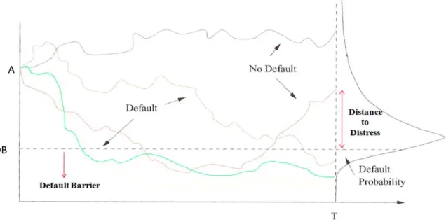
Default whenever the value of its implied assets—derived from market information on the liabilities and the Black and Scholes option pricing formula—falls below a default barrier. The difference between the asset value and the default barrier, scaled by the asset volatility, is referred to as the distance-to-default, while the area of the distribution that falls below the default barrier represents the firm’s default probability.

Figure 1: Default Interpretation in the Classical Merton Approach

Figure 1 shows several possible paths of firm value. Default occurs if the firm value at maturity is less than the default barrier. The particular path the firm value has taken does not matter here, only the firm value at time

T

is important. The probability of default therefore is equal to the probability that the firm value is below default barrier at time

T

. To calculate the probability, assumptions has to be made about the distribution of firm value at time

T

. The standard assumption is that firm value is log-normally distributed. The probability of default then is given as the area under the log-normal firm value density between zero and default barrier. This probability can be calculated explicitly in terms of

DB

, the current firm value

A

, the volatility of firm value, the risk-free interest rate and time.

III.2 The Borrower's Payoff from Loans

The total market value of assets,

A

, of a firm financed with debt,

D

, and equity,

E

, is equal to the market value of equity plus market value of risky debt. Asset value is derived from the

A 

stochastic discounted present value of income minus expenditures with the potential for asset value to decline below the point where scheduled debt payments can be made. If assets fall to or below this level, then default is the result. This level is often referred to as default barrier,

( )

DB

and represents the default-free value of debt. The holders of equity are holders of a junior claim and have a contingent claim on the residual value of assets in the future. In this approach, the value of equity can be viewed as an option where holders of equity receive the maximum of either assets minus debt, or nothing in the case of default. The value of equity, therefore, is,

(

A

DB

,

0

)

MAX

E

=

−

If the investments turn out badly, the stockholder - owners of the firm- would default on the firms debt, turn its assets

( )

A

over to the debt holders, and lose only their initial stake in the firms. By contrast, if the firm does well and the assets of the firm are valued highly

( )

A

, the firm's stockholders would payoff the firm's debt

( )

DB

and keep the difference

(

A

−

DB

)

.

III.3 The Debtholder's Payoff from Loans

Holders of debt are obligated to absorb losses if there is a default and the guarantee of repayment by the lender can be modeled as an implicit put option (i.e., in the event of default, the bondholders have a right to sell the remaining assets of the firm). Thus, holders of risky debt receive either the default free value or, in the event of default, the senior claim on assets. Beginning with the relationship between risky and default-free debt, this can be modeled as, Value of default-free debt = Value of risky debt + Value of the guarantee,

Since the value of default-free debt is the default barrier and the implicit put option on the assets of the firm yields

MAX

(

DB

−

A

,

0

)

( )

DB

, the market value of risky debt can be modeled as

(

A

,

DB

)

DB

MAX

(

DB

A

,

0

)

MIN

D

=

=

−

−

The maximum amount the bank or bondholder can get back is

DB

, the promised payment. However, the borrower who possesses the default or repayment option would only rationally repay the loan if

A

>

DB

. A borrower whose asset value falls below

DB

would default and turn over any remaining assets to the debt holders. Thus the value of the loan from the perspective of the lender is always the minimum of

DB

or

A

, or

MIN

(

DB

,

A

)

. That is, the payoff function to the debt holder is similar to writing a put option on the value of the borrowers' assets with

DB

as the exercise price.

III.4 Option Pricing Models

III.4.1 Black -Scholes Model

The Black-Scholes formula is an expression for the current value of a European call option on a stock which pays no dividends. The assumptions of the model are follows:

1. The stock price distributes log-normally and stock return distributes normally with

μ

and constant

σ

.

2. There are no riskless arbitrage opportunities 3. The short selling of securities is permitted. 4. There are no transactions costs and taxes.

5. There are no dividends during the life of the derivative. 6. Security trading is continuous.

III.4.1.1 Distribution of Stock Prices

The model of stock price behavior used by Black, Scholes and Merton assumes that percentage change in the stock price in a short period of time is normally distributed. Define:

μ

: Expected return on a stock

σ

: Volatility of the stock price

The mean of the percentage change in time

δ

t

is

μδ

t

and standard deviation of this percentage change is

σ

δ

t

, so that

S

S

δ

is distributed

N

(

μδ

t

,

σ

δ

t

)

where

δ

S

is the change in the stock price

S

in time

δ

t

.

( )

ln

( )

0

ln

S

_T

−

S

is distributed

⎥

⎦

⎤

⎢

⎣

⎡

⎟⎟

⎠

⎞

⎜⎜

⎝

⎛

−

T

T

N

μ

σ

,

σ

2

2

⎟⎟

⎠

⎞

⎜⎜

⎝

⎛

0

ln

S

S

_T is distributed

⎥

⎦

⎤

⎢

⎣

⎡

⎟⎟

⎠

⎞

⎜⎜

⎝

⎛

−

T

T

N

μ

σ

,

σ

2

2 (1) and

( )

S

T

ln

is distributed

⎥

⎦

⎤

⎢

⎣

⎡

⎟⎟

⎠

⎞

⎜⎜

⎝

⎛

−

+

T

T

S

N

μ

σ

,

σ

2

ln

2 0 ₍₂₎

where

S

_T is the stock price at a future time

T

and

S

₀is the stock price at time zero. Equation 2 shows that

ln

( )

S

_T is normally distributed. This means that

S

_T has a lognormal distribution.

III.4.1.2 Binomial Tree, Risk Neutral Valuation and No Arbitrage Argument

The Black-Scholes assumes that there are no riskless arbitrage opportunities. This assumption can be proved by setting up a portfolio which consists of a stock and option in such a way that there is no uncertainty about the value of the portfolio at the end of maturity. Because the portfolio has no risk, the return it earns must equal the risk-free rate. This enables to work out the cost of setting up the portfolio and therefore the option’s price. Because there are two securities and only two possible outcomes, it is always possible to set up the riskless portfolio.

Suppose that the option lasts for time

T

and that during the life of the option the stock price can either move up from

S

0to a new level

S

0

u

or down from

S

0to a new level

S

0

d

where

1

>

u

and

d

<

1

. If the stock price moves up to

S

₀

u

, the payoff from the option is

f

_u ; if the stock prices moves down to

S

₀

d

, the payoff from the option is

f

_d.

S0u

f

_u S₀

f

S₀d f_d

Consider a portfolio consisting of a long position in

Δ

shares of the stock and a short position in one call option. If there is an up movement in stock price, the value of the portfolio at the end of the life of the option is

S

0

u

Δ

−

f

u

If there is a down movement in the stock price, the value becomes

S

0

d

Δ

−

f

d

The two are equal

S

0

u

Δ

−

f

u=

S

0

d

Δ

−

f

d and

d

S

u

S

f

f

_{u d} 0 0

−

−

=

Δ

In this case, the portfolio is riskless and must earn the risk-free interest rate. If

r

is denoted as risk free interest rate, the present value of the portfolio is

S

₀

u

Δ

−

f

_u

e

−rT The cost of setting up the portfolio is

S

₀

Δ

−

f

It follows that

S

₀

u

Δ

−

f

_u

e

−rT

=

S

₀

Δ

−

f

or

f

=

S

₀

Δ

−

(

S

₀

u

Δ

−

f

_u

)

e

−rT Substituting for

Δ

, this equation reduces to

[

u

(

)

d

]

rT

f

p

pf

e

f

=

−

+

1

−

(3) where

d

u

d

e

p

rT

−

−

=

₍₄₎

p

is the probability of an up movement in the stock price. The variable

1

−

p

is then the probability of a down movement, and the expression

f

=

[

pf

u

+

(

1

−

p

)

f

d

]

is the expected payoff from the option. With this interpretation of

p

, equation 3 states that the value of the option is its expected future value discounted at the risk free interest rate.

When the probability of an up movement is assumed to be

p

, the expected stock price

( )

S

T

E

at time

T

is given by

( )

S

pS

u

(

p

)

S

d

E

_T

=

₀

+

1

−

₀ or

( )

S

pS

(

u

d

)

S

d

E

_T

=

₀

−

+

₀

Substituting from equation 4 for

p

,

( )

rT

T

S

e

S

E

=

₀

This equation shows that the stock price grows on average at the risk-free interest rate. Setting the probability of the up movement equal to

p

is therefore equivalent to assuming that the return on the stock equals to risk free rate.

In a risk neutral world all individuals are indifferent to risk. In such a world investors require no compensation for risk and the expected return on all securities is the risk-free interest rate. Equation 3 shows that the value of the option is its expected payoff in a risk-neutral world discounted at the risk free rate.

The logarithm of the expected return relative over a period of length one is now

r

, whereas it was

μ

under the original probability distribution. The risk-adjusted probability distribution has the property that the current value of any stock-price contingent claim equals the riskless discounted value of the expected future payoff, when the expected payoff is computed using the adjusted probabilities. This principle leads to a theoretically simple and intuitive derivation of the Black-Scholes formula. Valuing the call option and its components is just a matter of computing the expected value of some functions of a normally distributed variable (the normally distributed random variable beingln

( )

S_T ).

Risk adjustment of the probabilities in risk neutral world consists in replacing

μ

by

r

, the riskless interest rate. The risk-adjusted probability distribution is such that

S

_T is still log normally distributed, but the mean of the normally distributed variable

ln

( )

S

_T changes.

Replacing

μ

by

r

in equations 1 and 2

⎟⎟

⎠

⎞

⎜⎜

⎝

⎛

0

ln

S

S

_T is distributed

⎥

⎦

⎤

⎢

⎣

⎡

⎟⎟

⎠

⎞

⎜⎜

⎝

⎛

−

T

T

r

N

σ

,

σ

2

2 and

( )

S

T

ln

is distributed

⎥

⎦

⎤

⎢

⎣

⎡

⎟⎟

⎠

⎞

⎜⎜

⎝

⎛

−

+

r

T

T

S

N

σ

,

σ

2

ln

2 0

So, under the risk-adjusted probability distribution, the continuously compounded rate of return to the stock over a time interval of length one has variance,

σ

2 as before.

III.4.1.3 A Derivation of Black & Scholes Formula

The expected value of a European call option at maturity in a risk neutral world is

(

)

[

MAX

S

K

,

0

]

E

_T

−

(5)

where

S

_T is the stock price at maturity and K is the strike price of the option.

From the risk neutral valuation argument, the European call option price,

c

, is this expected value discounted at the risk free rate of interest, that is

c

=

e

−rT

E

[

MAX

(

S

_T

−

K

,

0

)

]

. (6) Expected value of

S

_T given that the option ends in the money can be calculated by using lognormal probability density function where

S

_T exceeds strike price

K

.

If a continuous variable

X

has a probability density function

f

( )

X

then it can be shown that its expected value is given by

E

( )

X

∫

Xf

( )

X

dx

+∞

∞ −

=

₍₇₎

If a continuous variable

X

is normally distributed with mean

μ

and variance

σ

2, then its probability density function is given by

( )

( ) 2 2 2 2

2

1

_σμ

πσ

− −

=

X

e

X

f

₍₈₎

Standard normal distribution is the normal distribution that has zero mean and unit variance. Setting

μ

=

0

and

σ

2

=

1

in equation 8, the probability density function for the standard normal distribution is

( )

2 2

2

1

X

e

X

f

−

=

π

(9)

If X is normally distributed with mean

μ

and variance

σ

2, X can always be converted into a standard normal

Z

variable by subtracting the mean from

X

and then dividing by standard deviation

σ

. That is

σ

μ

−

=

X

Z

_{distributed with mean zero and standard deviation 1. (10)}

It is already shown that

S

_T is log-normally and

ln

( )

S

_T is normally distributed.

( )

S

T

ln

is distributed

⎥

⎦

⎤

⎢

⎣

⎡

⎟⎟

⎠

⎞

⎜⎜

⎝

⎛

−

+

r

T

T

S

N

σ

,

σ

2

ln

2 0 ₍₁₁₎

( )

S

T

ln

can be converted into a standard normal

Z

variable by using equation 10.

s

m

S

Z

=

ln

T

−

where

m

is mean and

s

is the standard deviation of

ln

( )

S

_T . (12) The new variable

Z

is normally distributed with mean zero and standard deviation 1. The probability density function for

Z

is

( )

2 2

2

1

Z

e

Z

f

−

=

π

(13)

Equation 7 shows that

(

)

[

]

(

) ( )

T T K T T

K

S

K

f

S

dS

S

MAX

E

∫

∞

−

=

−

,

0

₍₁₄₎

By using equation 12 to convert the expression on the right hand side of the equation 14 from an integral over

S

_T to an integral over

Z

, it is obtained

(

)

[

]

_∫

∞

(

)

( )

− +

₋

=

−

s m K m Zs T

K

e

K

f

Z

dz

S

MAX

E

ln

0

,

(15)

[

(

)

]

∫

( )

∫

( )

∞ − ∞ − +

₋

=

−

s m K s m K m Zs T

K

e

f

Z

dz

Kf

Z

dz

S

MAX

E

ln ln

0

,

( )

_∫

( )

∫

∞ − ∞ − +

₋

=

s m K s m K m Zs

dz

Z

f

K

dz

Z

f

e

ln ln

∫

∫

∞ − − ∞ − − +

₋

=

s m K Z s m K Z m Zs

dz

e

K

dz

e

e

ln 2 ln 2 2 2

2

1

2

1

π

π

(

)

∫

∫

∞ − − ∞ − + + −

−

=

s m K Z s m K m Zs Z

dz

e

K

dz

e

ln 2 ln 2 2 2 2 2

2

1

2

1

π

π

( )

[

]

∫

∫

∞ − − ∞ − + + − −

−

=

s m K Z s m K s m s Z

dz

e

K

dz

e

ln 2 ln 2 2 2 2 2

2

1

2

1

π

π

( )

(

)

∫

∫

∞ − − ∞ − + − −

−

=

s m K Z s m K s m s Z

dz

e

K

dz

e

e

ln 2 ln 2 2 2 2 2 2

2

1

2

1

π

π

(

)

( )

∫

∫

∞ − − ∞ − − − +

−

=

s m K Z s m K s Z s m

dz

e

K

dz

e

e

ln 2 ln 2 2 2 2 2 2

2

1

2

1

π

π

(16)

If

N

( )

X

is defined as the probability that a variable with a mean zero and standard deviation of 1 is less than

X

, integral of the equation 16 is

(

)

⎭

⎬

⎫

⎩

⎨

⎧

⎥

⎦

⎤

⎢

⎣

⎡

⎟

⎠

⎞

⎜

⎝

⎛

−

−

−

⎭

⎬

⎫

⎩

⎨

⎧

⎥

⎦

⎤

⎢

⎣

⎡

₋

⎟

⎠

⎞

⎜

⎝

⎛

−

−

=

+

s

m

K

N

K

s

s

m

K

N

e

s m

ln

1

ln

1

2 2 2

(

)

⎥

⎦

⎤

⎢

⎣

⎡

⎟

⎠

⎞

⎜

⎝

⎛

−

−

−

⎥

⎦

⎤

⎢

⎣

⎡

⎟

⎠

⎞

⎜

⎝

⎛

−

−

=

+

s

m

K

KN

s

m

K

s

N

e

s m

ln

ln

2 2 2

Substituting for m and s from equation 11 gives,

⎥

⎥

⎥

⎥

⎥

⎦

⎤

⎢

⎢

⎢

⎢

⎢

⎣

⎡

−

⎟⎟

⎠

⎞

⎜⎜

⎝

⎛

−

+

−

⎪

⎪

⎭

⎪

⎪

⎬

⎫

⎪

⎪

⎩

⎪

⎪

⎨

⎧

⎥

⎥

⎥

⎥

⎥

⎦

⎤

⎢

⎢

⎢

⎢

⎢

⎣

⎡

⎟⎟

⎠

⎞

⎜⎜

⎝

⎛

−

−

−

−

=

⎟⎟⎠ + ⎞ ⎜ ⎜ ⎝ ⎛ − +

T

K

T

r

S

KN

T

T

r

S

K

T

N

e

T T r S

σ

σ

σ

σ

σ

σ σ

ln

2

ln

2

ln

ln

2 0 2 0 2 2 ln ₀ 2 2

⎥

⎥

⎥

⎥

⎥

⎦

⎤

⎢

⎢

⎢

⎢

⎢

⎣

⎡

⎟⎟

⎠

⎞

⎜⎜

⎝

⎛

−

+

−

⎪

⎪

⎭

⎪

⎪

⎬

⎫

⎪

⎪

⎩

⎪

⎪

⎨

⎧

⎥

⎥

⎥

⎥

⎥

⎦

⎤

⎢

⎢

⎢

⎢

⎢

⎣

⎡

⎟⎟

⎠

⎞

⎜⎜

⎝

⎛

−

+

+

=

+

T

T

r

K

S

KN

T

T

r

K

S

T

N

e

S rT

σ

σ

σ

σ

σ

2

ln

2

ln

2 0 2 0 ln ₀

T

T

r

K

S

d

σ

σ

⎟⎟

⎠

⎞

⎜⎜

⎝

⎛

−

+

=

2

ln

2 0 2

(

)

[

MAX

S

K

,

0

]

S

₀

e

N

(

T

d

₂

)

KN

( )

d

₂

E

_T

−

=

rT

σ

+

−

(

)

[

MAX

S

K

,

0

]

S

0

e

N

( )

d

1

KN

( )

d

2

E

_T

−

=

rT

−

c

=

e

−rT

E

[

MAX

(

S

_T

−

K

,

0

)

]

c

=

S

₀

N

( )

d

₁

−

Ke

−rT

N

( )

d

₂ (17) III.4.1.4 Understanding

N

( )

d

₁ and

N

( )

d

₂

The Black and Scholes formula expresses the call value as the current stock price times a probability factor

N

( )

d

₁ , minus the discounted exercise price times a second probability factor

( )

d

2

N

.

Among the major research papers, Black and Scholes (1973) did not explain or interpret

( )

d

1

N

and

N

( )

d

₂ . Neither did Merton (1973, 1990), Cox and Ross (1976), or Rubinstein (1976). As for the textbooks, Jarrow and Rudd (1983) derive the Black-Scholes formula using risk-adjusted probabilities, and in the process they do interpret

N

( )

d

₁ and

N

( )

d

₂ . Cox and Rubinstein (1985) state that the stock price times

N

( )

d

₁ is the present value of receiving the stock if and only if the option finishes in the money, and the discounted exercise payment times

( )

d

2

N

is the present value of paying the exercise price in that event. They do not explain why this is so or relate it to the probability that the option finishes in the money. Hull (1989, 1991, 2002, 2006, 2009) do not explain

N

( )

d

₁ and

N

( )

d

₂ .

From the definition of a call option, the expected value of the call option at maturity is

[ ]

c

E

[

MAX

(

S

K

,

0

)

]

E

_T

=

_T

−

(18)

There are two possible situations that can happen at maturity. If

S

_T

>

K

, the call option expires in the money and

E

[

MAX

(

S

T

−

K

,

0

)

]

=

S

T

−

K

.

If

S

T

<

K

, the option

expires out of money and

E

[

MAX

(

S

_T

− K

,

0

)

]

=

0

.

If

p

is defined as the probability that

T

S

>

K

, equation 18 can be rewritten:

[ ]

c

=

p

×

(

E

[

S

S

>

K

]

−

K

)

+

(

1

−

P

)

×

0

[ ]

c

p

(

E

[

S

S

K

]

K

)

E

_T

=

×

_{T T}

>

−

where:

p

is the probability that

S

_T

>

K

[

S

S

K

]

E

_{T T}

>

is the expected value of the call option at maturity.

Finding the probability

p

that stock price at maturity

S

_T will exceed some critical price

K

is the same as finding the probability that the return of the stock over the period will exceed some critical value.

[

S

T

K

]

ob

[

turn

S

turn

Critical

]

ob

p

=

Pr

>

=

Pr

Re

>

Re

[

]

⎥

⎦

⎤

⎢

⎣

⎡

⎟⎟

⎠

⎞

⎜⎜

⎝

⎛

>

⎟⎟

⎠

⎞

⎜⎜

⎝

⎛

=

>

=

0 0

ln

ln

Pr

Pr

S

K

S

S

ob

K

S

ob

p

T T

In Black Scholes model,

⎟⎟

⎠

⎞

⎜⎜

⎝

⎛

0

ln

S

S

T

is assumed normally distributed.

⎟⎟

⎠

⎞

⎜⎜

⎝

⎛

0

ln

S

S

_T is distributed

⎥

⎦

⎤

⎢

⎣

⎡

⎟⎟

⎠

⎞

⎜⎜

⎝

⎛

−

T

T

r

N

σ

,

σ

2

2

[

]

[

]

⎟⎟

⎠

⎞

⎜⎜

⎝

⎛

−

−

=

>

=

>

=

turn turn crit Critical S T

turn

N

turn

turn

ob

K

S

ob

p

Re Re

Re

1

Re

Re

Pr

Pr

σ

μ

[

]

⎟

⎟

⎟

⎟

⎟

⎠

⎞

⎜

⎜

⎜

⎜

⎜

⎝

⎛

⎟⎟

⎠

⎞

⎜⎜

⎝

⎛

−

−

⎟⎟

⎠

⎞

⎜⎜

⎝

⎛

−

=

>

=

T

T

r

S

K

N

K

S

ob

p

_T

σ

σ

2

ln

1

Pr

2 0

[

]

⎟

⎟

⎟

⎟

⎟

⎠

⎞

⎜

⎜

⎜

⎜

⎜

⎝

⎛

⎟⎟

⎠

⎞

⎜⎜

⎝

⎛

−

−

⎟⎟

⎠

⎞

⎜⎜

⎝

⎛

−

=

>

=

T

T

r

S

K

N

K

S

ob

p

_T

σ

σ

2

ln

Pr

2 0

[

]

⎟

⎟

⎟

⎟

⎟

⎠

⎞

⎜

⎜

⎜

⎜

⎜

⎝

⎛

⎟⎟

⎠

⎞

⎜⎜

⎝

⎛

−

+

−

=

>

=

T

T

r

K

S

N

K

S

ob

p

_T

σ

σ

2

ln

ln

Pr

2 0

[

]

⎟

⎟

⎟

⎟

⎟

⎠

⎞

⎜

⎜

⎜

⎜

⎜

⎝

⎛

⎟⎟

⎠

⎞

⎜⎜

⎝

⎛

−

+

⎟

⎠

⎞

⎜

⎝

⎛

=

>

=

T

T

r

K

S

N

K

S

ob

p

_T

σ

σ

2

ln

Pr

2 0

p

=

Pr

ob

[

S

T

>

K

]

=

N

( )

d

2 (19) and

N

( )

d

₁

=

N

(

σ

T

+

d

₂

)

( )

d

2

N

is the risk-adjusted probability that the option will be exercised. But, the present value of contingent receipt of the stock is not equal to but larger than the current stock price multiplied by

N

( )

d

₂ , the risk-adjusted probability of exercise. The reason for this is that the event of exercise is not independent of the future stock price. If exercise were completely random and unrelated to the stock price, then indeed the present value of contingent receipt of the stock would be the current stock price multiplied by

N

( )

d

₂ . Actually the present value is larger than this, since exercise is dependent on the future stock price and indeed happens when the stock price is high.

The expected value, computed using risk-adjusted probabilities, of receiving the stock at expiration of the option, contingent upon the option finishing in the money, is

N

( )

d

₁ multiplied by the current stock price and the riskless compounding factor. Thus,

N

( )

d

₁ is the factor by which the present value of contingent receipt of the stock exceeds the current stock price.

III.4.2 The Gram-Charlier Model

The basic assumption of the Black–Scholes framework is that the returns of the assets are normally distributed. In other words skewness

( )

ξ

and kurtosis

( )

κ

of the returns are zero and three respectively. However, the real probability distributions of the returns may present heavy tails and asymmetry in the market. Excess kurtosis indicates more weights in both tails of the distribution than in normal distribution. In other words heavy-tailed probability densities have higher weight around the mean as well as more weight in the tails. If the returns have excess kurtosis, the probability of large negative or large positive values is greater than the normal probability density function. So the lower quantiles are less than the normal quantiles and the upper quantiles are greater. When there is excess kurtosis in stock returns, Gram-Charlier expansion can be used effectively which allows for additional flexibility over the normal probability density function because it introduces the skewness and kurtosis of the empirical distribution as parameters. A Gram-Charlier expansion generates a density function for a standardized random variable that differs from the standard normal in having nonzero skewness and excess kurtosis.

A Gram-Charlier expansion defines a density for

Z

by

( )

⎟

⎠

⎞

⎜

⎝

⎛

₋

₊

=

(

)

24

6

1

)

(

)

(

3 4

Z

f

Z

f

Z

f

Z

ξ

κ

φ

where

s

m

S

Z

=

ln(

T

)

−

_{is a standard normal variable distributed with}

_m

_and

_s

_,

2 2

2

1

)

(

Z

e

Z

f

−

Π

=

_{is the standard normal probability density function,}

_f

( )k

( )

_x

denotes the

k

th derivative of

f

( )

x

.

Backus, Foresi and Wu (2004) showed that price of a call option on a non dividend paying stock is given by,

[

(

)

]

(

)

( )

(

∫

) ∞ − + − −

₋

₌

₋

=

s m K m Zs rT T rT

dZ

Z

K

e

e

K

S

MAX

E

e

c

ln

0

,

φ

₍

(

₎

)

( )

₍

( )

₎

dZ

Z

Ke

dZ

Z

K

e

e

c

s m K rT s m K m Zs rT

∫

∫

∞ − − ∞ − + −

₋

₋

=

ln ln

φ

φ

Straja (2001) demonstrated that exact price of a call option on a non dividend paying stock which takes into account the skewness and kurtosis is

( )

(

)

(

)

(

d

T

)

Ke

T

T

e

d

d

T

T

d

T

T

e

d

S

c

rT T T T T

σ

φ

κ

σ

ξ

σ

κ

σ

σ

ξ

σ

σ

φ

κ σ ξ σ κ σ ξ σ

−

−

⎪

⎪

⎪

⎪

⎪

⎭

⎪⎪

⎪

⎪

⎪

⎬

⎫

⎪

⎪

⎪

⎪

⎪

⎩

⎪⎪

⎪

⎪

⎪

⎨

⎧

⎟

⎠

⎞

⎜

⎝

⎛

₊

+

⎥

⎥

⎥

⎥

⎦

⎤

⎢

⎢

⎢

⎢

⎣

⎡

−

+

−

+

−

+

=

− − − − −

24

6

24

1

3

3

6

2

2 4 2 3 3 24 6 2 2 24 6 0 2 4 2 3 3 2 4 2 3 3 where,

T

T

T

T

r

K

S

d

σ

κ

σ

ξ

σ

σ

⎥

⎦

⎤

⎢

⎣

⎡

⎟

⎠

⎞

⎜

⎝

⎛

₊

−

⎟⎟

⎠

⎞

⎜⎜

⎝

⎛

+

+

⎟

⎠

⎞

⎜

⎝

⎛

=

2

6

24

ln

0 2 3 3₂ 4 2

φ

: cumulative normal probability density function

0

S

_{: stock price at time zero}

K

: exercise price

T

: time to maturity (expiration date) in terms of year

r

: continuously compounded annual risk free interest rate

σ

: annual volatility (standart deviation)

ξ

: skewness coefficient

κ

: kurtosis coefficient

III.5 Option Pricing Models and Probability of Default

Given that assets and liabilities in the firm balance sheet can be related using implicit options, the standard option pricing formula can be used to price these relationships. The main insight behind the methodology of the Black-Scholes formula is that the value of the option can be derived by forming a riskless hedge portfolio. A riskless portfolio is created consisting of a position in a derivative security and a position in a stock. The risk-free nature of the portfolio is derived from the fact that both the derivative and stock price are affected by the same underlying source of uncertainty. Over any short period of time, the two must be perfectly correlated. If the appropriate positions are established, the gain (loss) from the stock position always offsets the loss (gain) from the derivative security, so that the overall value of the position at the end of the period is known with certainty. Therefore, the return of the hedge portfolio is equal to the risk-free rate of interest. By forming a riskless hedge portfolio, the derivation relies primarily on no-arbitrage principles as opposed to equilibrium relationships. The return must be equal to the risk-free rate over the holding period.

Using the Black-Scholes formula, the value of equity as a call option on firm assets is,

( )

d

1

DBe

N

( )

d

2

AN

E

=

−

−rT (20)

where

A

is the value of the assets,

E

is the value of equity,

DB

is the default barrier or value of default-free debt,

r

is the risk-free rate of interest,

T

is the time to maturity on the defaultfree bond in years.

N

( )

d

is the cumulative probability distribution function for a standard normal