T.C.
ISTANBUL AYDIN UNIVERSITY
INSTITUTE OF SCIENCE AND TECHNOLOGY
M.Sc. THESIS
DECEMBER 2016
SPECTRUM SENSING DETECTION METHODS IN COGNITIVE RADIO SYSTEMS
Amir ESLAMI
Department of Electrical and Electronics Engineering Electrical and Electronics Engineering Program
DECEMBER 2016 T.C.
ISTANBUL AYDIN UNIVERSITY
INSTITUTE OF SCIENCE AND TECHNOLOGY
SPECTRUM SENSING DETECTION METHODS IN COGNITIVE RADIO SYSTEMS
MASTER OF SCIENCE THESIS Amir ESLAMI
Y1513.300006
Department of Electrical & Electronics Engineering Electrical and Electronics Engineering Program
v DECLARATION
I hereby declare that all information in this thesis document has been obtained and presented in compliance and confirmation to the ethical code of conduct and prescribed academic regulations. I also declare that as required by these rules and conduct, I have fully cited and referenced all the text and concepts that did not belong to me and were inferred from past researchers’ Works. (28/12./2016)
vii FOREWORD
This thesis is the final work of my study at Electrical and Electronics Engineering department of Istanbul Aydin University. This thesis serves the studies upon novel algorithms for cognitve radio based hospitals with using memory sticks in them. This thesis is the result of a hard work with Assist. Prof. Saeid Karamzafeh and we have reached perfect results comparing the ones exists in literature and published them to help the researchers to understand our ideas also.
December 2016 Amir Eslami
ix TABLE OF CONTENTS Page FOREWORD ... vii TABLE OF CONTENT... ... ix ABREVIATIONS ... xi SYMBOLS... ... xiii LIST OF TABLE ... xv
LIST OF FIGURE ... xvii
ÖZET... ... xix
ABSTRACT... ... xxi
1. INTRODUCTION ... 1
1.1 Cognitive Radio Technology In Cellular Networks ... 4
1.2 Cognitive Radio Based Hospitals ... 5
1.3 Spectrum Sensing ... 5
1.3.1 Matched filter ... 6
1.3.2 Cyclostationary feature detection ... 6
1.3.3 Energy detection ... 6
1.3.4 Eigen-value based detection ... 6
1.4 Environment model ... 7 2. CHANNEL MODELING ... 9 2.1 Large-sclae Fading ... 12 2.1.1 Okumara/Hata Model ... 16 2.1.2 COST 231 model ... 17 2.1.3 Walfisch/Bernoti Model ... 18
2.2 Small Scale Fading ... 19
2.2.1 Flat fading ... 19
2.2.2 Frequency selective fading ... 20
2.3 Well known Fading Channels ... 20
2.3.1 Rayleigh fading ... 21
2.3.2 Nakagami-m fading ... 21
3. SYSTEM MODEL AND SPECTRUM SENSING ALGORITHMS ... 25
3.1 Energy Detetion Based Spectrum Seninge Algorithms ... 26
3.1.1 Classical energy detection ... 26
3.1.2 Double threshold energy detection based spectrum sensing method ... 32
3.2 Covariance Based Spectrum Sensing ... 37
3.2.1 Maximum to minimum eigen-value based spectrum sensing ... 43
3.2.2 Energy to minimum eigen-value based spectrum sensing ... 44
3.2.3 Double threshold maximum to minimum eigen-value spectrum sensing Method ... 47
4. MEMORY CONCEPT IN COGNITIVE RADIO DRIVEN HOSPITALS SENSING ALGORITHMS ... 51
x
4.1 Memory Based Double Threshold Energy Detection Spectrum Sensing
Algorithm ... 51
4.2 Memory based energy detection spectrum sensing algorithm ... 56
5. CONCLUSION ... 61
REFERENCES ... 63
xi ABREVIATIONS
DSP : Digital Signal Processing CR : Conitive Radio
USA : United States of America
UK : United Kingdom
FCC : Federal Communications Commission IID : Independent and identically distributed ED : Energy Detection
NU : Noise Uncertainty
DTED : Double Threshold Energy Detection DOA : Direction Of Arrival
EME : Energy to Minimum Eigen-value MME : Maximum to Minimum Eigen-value GHz : Giga Hertz
TV : Television
HF : High Frequency UHF : Ultra High Frequency SHF : Super High Frequency
MHz : Mega Hertz
PDF : Probability Density Function BPSK : Binary Phase Ahift Keying
QPSK : Quadrature Probability Phase Shift Keying RAC : Restricted Area Constant
MBED : Memory Based Energy Detection
xiii SYMBOLS Fc : Carrier frequency τn : Delay fD,n : Doppler effect Pt : Transmit power Gt : Transmit gain Gr : Reciever gain
L : System loss factor
d : Distance
n : Path loss exponent 𝝈 : Shadowning effect.
AMU(f,d) : Medium attenuation factor
hRx : Height of transmitter antenna.
hTx : Height of reciever antenna.
CRx : Correlation coefficient of the receiver antenna
P0 : omnidirectional antennas free space path loss
Q2 : Signal power reduction
Bc : Coherence bandwidth
Ts : symbol period
𝝈η : Noise variance
λ : Energy detection threshold Pfa : Probability of false alarm
Pd : Probability of detection
θ : Restricted area constant
Ri : Decision
xv LIST OF TABLES
Page
Table 2.1 : Path loss exponent values for different environments. ... 14 Table 3.1 : Tracy-Widom distribution table for some samples ... 43
xvii LIST OF FIGURE
Page
Figure 1.1 : United States of America Frequency Allocation. ... 2
Figure 1.2 : United Kingdom Frequency Allocation. ... 2
Figure 1.3 : New Zealand Spectrum allocation... 3
Figure 1.4 : Spectrum utilization measurement up to 6 MHz. ... 4
Figure 2.1 : Wireless Channel effects. ... 9
Figure 2.2 : Fading phenomena classifications ... 11
Figure 2.3 : Baseband communication system. ... 11
Figure 2.4 : Channel effects in wireless channels ... 12
Figure 2.5 : Free space path loss model with fc = 1.5 GHz... 13
Figure 2.6 : Log-distance path loss model with fc = 1.5 GHz. ... 15
Figure 2.7 : Log-normal Shadowing path loss model with fc = 1.5 GHz. ... 16
Figure 2.8 : Hata path loss model with fc = 1.5 GHz. ... 18
Figure 2.9 : Rayleigh fading pdf with different. ... 22
Figure 2.10 : Nakahami-m distribution PDF with different m values. ... 23
Figure 3.1 : Energy Dection based spectrum sensing performance comparison with BPSK, QPSK and 8 PSK modulations. ... 29
Figure 3.2 : Energy Detection based spectrum sensing performance comparison with different signal types such as rectangular, raised cosine and root raised cosine types. ... 30
Figure 3.3 : Energy detection sensing method performance of QPSK in Gaussian, Rayleigh and Nakagami-m fading channels with m=1, 2 and 15. ... 30
Figure 3.4 : Energy Detection based spectrum sensing method’s performance with 0, 0.5, 1, 1.5 and 2dB noise uncertainty for signal passing through Gaussian channel. ... 31
Figure 3.5 : Energy detection based spectrum sensing method performance with 0, 0.5, 1, 1.5 and 2dB noise uncertainty for signal passing through Rayleigh channel. ... 31
Figure 3.6 : Percentage of the energy samples used to make decision using double threshold energy detection method with RAC=0.5 in different channels. ... 34
Figure 3.7 : Percentage of the valuable energy samples eliminated using double threshold energy detection method with RAC=0.5 in different channels ... 34
Figure 3.8 : Percentage of the energy samples used in double threshold energy detction method with RAC = 0.25,0.5 and 0.75 in Gaussian channel. . 35
Figure 3.9 : Percentage of the valuable energy samples eliminated using double threshold energy detection method with RAC= 0.25, 0.5 and 0.75in Gaussian channel ... 35
xviii
Figure 3.10 : Double threshold energy detection method with RAC = 0.5 performance comparison in different channels. ... 36 Figure 3.11 : Double threshold energy detection method with RAC = 0.25, 0.5 and 0.75 and Noise Uncertainty = 0, 1 and 2 dBs performance comparison in Gaussian channel. ... 36 Figure 3.12 : A model of wireless communication. ... 38 Figure 3.13 : Energy detection, double threshold energy detection, maximum to minimum eigen value and EME sensing method performance comparison of QPSK modulation in Gaussian channel. ... 46 Figure 3.14 : Double threshold maximum bto minimum eigen-value, maximum to minimum eigen-value and energy detection sensing method algorithms with 0,1 and 2 dB uncertainties passing through Gaussian channels.... 49 Figure 3.15 : Double threshold maximum bto minimum eigen-value, maximum to minimum eigen-value and energy detection sensing method performance with 0, 1 and 2 dB uncertainties passing through Rayleigh channel. ... 50 Figure 3.16 : Double threshold maximum to minimum eigen-value sensing method performance in different channels... 50 Figure 4.1 : Energy detection, double threshold energy detection and memoryful double threshold energy detection sensing methods performance over Gaussian channel. ... 54 Figure 4.2 : Energy detection, double threshold energy detection and memory based double threshold energy detection sensing methods performance over Rayleigh channel ... 55 Figure 4.3 : Memory based double threshold energy detection sensing method performance without memory and memory of saving 1 and 2 previously sensed signals energy over Gaussian channel ... 55 Figure 4.4 : Memory based double threshold energy detection sensing method performance without memory and memory of saving 1 and 2 previously sensed signals energy over Rayleigh channel. ... 56 Figure 4.5 : Energy detection, double threshold energy detection and memory based energy detection sensing methods performance over Gaussian channel. ... 58 Figure 4.6 : Energy detection, double threshold energy detction and memory based energy detction sensing methods performance over Nakagami-15 channel. ... 59 Figure 4.7 : Energy detection, double threshold energy detction and memory based energy detction sensing methods performance over Rayleigh channel 59 Figure 4.8 : Performance comparison of memory based energy detection sensing method over Nakagami-m channels. ... 60
xix
KAVRUMSAL RADYO SİSTEMLERİNDE SPEKTRUM ALGILAMA METODLARI
ÖZET
Hastanelerde uzaktan bağlantıyı sağlamak ve çok fazla miktardaki kabloları kaldırmanın kilit teknlojisi, kablosuz iletişim teknolojisidir. Ama kablosuz cihazların artması ile spektrum bant aralığı yetersiz kalıyor. Kavrumsal radyo bazlı hastaneler spektrum eksikliğini çözmek için literaturde tanıtılmıştır. Kavrumsal radyo yüksek data hız ihtiyacından oluşan spektrum eksikliğini çözmek için en etkili teknolojidir. Kavrumsal radyo teknolojisinde lisans sahibi olmayan kullanıcılara, lisanlı kullanıcının bant aralığının kullanmadığı zamanlarda kullanım imkani sunar. Lisans sahibi kullanıcı, bant aralığını kullanmaya başadığı anda, linaslı olmayan kullanıcı data göndermeyi durdurur ve lisanslı kullanıcının veri aktarımının bitmesini bekler. Kavrumsal radyo bazlı hastanelerde, cihazlar, baz istasyonlu iletişimde olduğu gibi iki kategoriye ayrılır. Birincil cihazlar, hastanede lisanslı cihazlar gibi olup, iletişimleri hayati öneme sahip olanlardır. İkincil cihazlar, hastanede liansı olmayan cihazlar gibi olup, az öneme sahiplerdir ve iletişimleri bekleye bilir. Kavrumsal radyoda bazlı hatanelerde en önemli parametre, spektrumun kullanılıp kullanılmadığına doğru karar vermesidir. Pek çok spektrum algılama metodu bulanmaktadır ama enerji bazlı algılama ve kovariyans tabanlı spektrum algılama en ünlü metodlardır. en yüksek bölü en düşük özdeğer metodu, kovarians tabanlı spektrum algılama konseptinde en iyi tanınan metod dur. Enerji bazlı algılama metodunun performansını yükseltmek için, çift eşik konsepti tanımlanmıştır. Literatürde çift eşik enerji bazlı algılama metodu, enerji bazlı spektrum algılama metodunun performansını artırmak için sunulmuştur. Bu tezde, çift eşik konseptini en yüksek bölü en düşük özdeğer metoduna uygulayarak , çift eşik bazını en çok tanınan kovarians bazlı spektrum algılama metodunu tanıttık. Bu metod, karmaşıklığı yüzünden, kavrumsal radyo bazlı hastanelerde kullanılamıyor. Literatürde tanımlanan başka bir yöntem ise işbirlikli algılama dir ki bu yöntem, cihazların algılama parçalarını artırıp, kablolar kullandığı için kavrumsal radyo bazlı hastanelerde kullanılamaz. Biz bu tez çalışmasında, bellek konseptini tanıtıp, bu konsepti kullanarak iki algılama algoritma ürettik. Bellek konsepti, ikincil cihazların iletişim gecikmesini kullanarak, algılama performansı çok yüksek derecede artırıyor. ikincil cihazların iletişim gecikmesi kabul edilebilir bir parametredir. Bu algoritmalar, bellek bazlı çift eşik enerji algılaması ve bellek bazlı enerji algılama metodlarıdır. Bu metodların her biri kendine özel artıları ve eksileri vardır.
Anahtar Kelimeler : Kavrumsal radyo, Enerji bazlı spektrum algılama, Çift eşik bazlı spektrum algılama, Kavrumsal radyo bazlı hastane, bellek bazlı çift eşik spektrum algılama, bellek bazlı enerji algılama.
xxi
SPECTRUM SENSING DETECTION METHODS IN COGNITIVE RADIO SYSTEMS
ABSTRACT
Wireless technology is the key technology to eliminate the dense wire ropes from hospitals and far access to medical devices. In order to overcome the problem of bandwidth scarcity, cognitive radio driven hospitals are introduced. Cognitive radio is the most effective technology to solve spectrum scarcity problem in contrast to high speed data transfer need. In cognitive radio systems, non-licensed users are permitted to use an idle licensed spectrum bandwidth. Whenever the license holder begin to use its spectrum, non-licensed user stops its communication and waits until the licensed user finish its communication. In cognitive radio driven hospitals, devices are divided in two categories just as the one in cellular communication. Primary devices has very high priority and their communication is vital for the hospital and patients, so that no interference should be made with such devices. Secondary devices are the ones which has lower priority and they can wait until the primary devices do their communication and then, they begin to use the allocated spectrum. The most important parameter in cognitive radio driven hospitals is a reliable spectrum sensing method. This method should be a simple one to be able to implement it in the secondary devices. Among all the sensing methods, energy detection based spectrum sensing and covariance based spectrum sensing is very popular. Maximum to minimum eigen-value based spectrum sensing is the best known of the covariance based spectrum sensing. In order to improve the performance of energy detection, double threshold concept is introduced. Double threshold energy detection method is introduced in literature to improve energy detection method performance. In this thesis, we used this concept in maximum to minimum eigen-value based spectrum sensing to improve its performance. The problem with covariance based spectrum sensing is its complexity. These complex methods can not be used in real systems of cognitive radio driven hospitals. The other method to improve the sensing algorithms performance is cooperative concept. The main reason of wireless hospitals is eliminating complexity and dense ropes that by using cooperative system for the devices, again this ropes and complexity will be used again. We have suggested to use memory concept in energy detection based spectrum sensing methods. Two new algorithms are introduced with considerably better performance with the cost of delay in secondary communication which is bearable. These new methods are memory based double threshold energy detection and memory based energy detection with their pros and cons.
Keywords: Cognitive radio, Energy based spectrum sensing, Double threshold Energy based spectrum sensing, Cognitive radio based hospitals, Memory based double threshold energy detection, Memory based energy detection.
1 1. INTRODUCTION
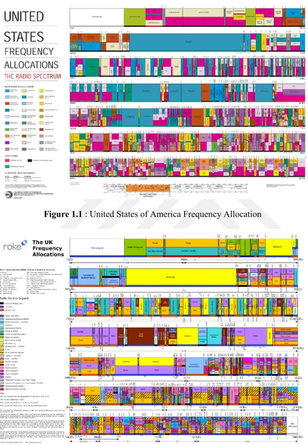
In these days many business fields depend on the radio spectrum usage such as narrow and broadband mobile telecommunications, medical researches, marine communications, scientific researches and emergency services. Thus radio services and communications are important for evolution of sience and economics which has made the radio spectrum an important natural resource recently. The development of new wireless technologies and various services has made the usage of this natural resource in such a high range that recently all industrial fields are using this technology in their production lines. Digital signal processing (DSP) is the key technology led up wireless communication to become such a sucessful technology. DSP arose due to endless efforts of leaders such as Alan Oppenheim [1], James Flangan [2], Fred Harris [3], Ronald Schaefer [4], James McClellen [5],[6] and many others. These pioneers has prepared innovative papers and books to teach how to convert analog signal processes to digital ones to be used in industaries. Following the Moore’s law [7] in semicondoctor industury had let the complex computational performance needed to implement DSP techniques to be practically possible. This caused to use digital functions implemented in silicons to be replaced with analog functions implemented with large discrete components and made the systems more reliable ,flexible, smaller and cheaper for the customer. By developing such a small and reliable components, many softwares and algorithms were designed and introduced to expand this revelotionary invention more. On the other hand using the radio spectrm as the physical layer for trancivering data, and demand for higher speeds of data transferring has caused the spectrum bands to be overused in a way that this resource has become an scarce one recently [8]. The key function should be addressed in wireless technology is the access to radio spectrum bands. Interference management and access control are the main duties of spectrum management, as the spectrum is allocated by governemental or non-governemental agencies, the capacity to manage interference become an important factor to increase the number of users. Allocation of spectrum is done by individual nation determined organizations and international agreements. Figure 1.1 shows the spectrum allocation for United States of America and figure 1.2
2
shows the spectrum alloation for United Kingdom for the frequency band in entire nation [9]. Each color represents a service in the region.
Figure 1.1 : United States of America Frequency Allocation
3
Figure 1.3 shows the spectrum allocation in New Zealand country [10]. The intensity of services in USA and UK, frequency allocation is noticeably more than the one in New Zealand because they provide more services for commercial and non commercial organizations such as scientific researches , air traffic and defense technologies.
Figure 1.3 : New Zealand Spectrum allocation
Studies has shown that most of the allocated licensed spectrum is underutilized in space and time domain. These unused frequncy bands are named white spaces in this project. Federal Communications Commission (FCC) has reported the temporal and geographic variations in spectrum utilization is range from 15% to 85% [11]. Spectrum utilization in figure 1.3 shows that the spectrum utilization is mainly is more intense in the frequencies below 3 GHz and it is less betwwen the frequencies between 3-6 GHz spectrum bands.
It is so obvious that there is a big misutilization of spectrum band even though there is a big scarcity of spectrum. Figure 1.4 show the spectrum utilization measurement up to 6 Ghz [12]. Fixed spectrum allocation policy has forced wireless service operators use only the spectrum allocated to them even if the other spectrum bands are not used at the moment. Cognitive radio (CR) technology is introduced to mitigate the scarcity of spectrum by using these spectrum holes.
4
Figure 1.4 : Spectrum utilization measurement up to 6 GHz
Cognitive radio is the technology of intelligently detecting spectrum holes in a radio channel and using these spectrum holes by users not licensed for the spectrum band until the owner of spectrum begin using it again. This idea was pioneered by J. Mitola III [13] from software defined radio was considered to make spectrum utilization improved. This technology is mainly used in cellular communications [8] and wireless hospitals [16]. The most important aspect in CR systems is spectrum sensing to avoid collision in a reasonable range.
1.1 Cognitive Radio Technology in Cellular Networks
There are many service providers in a country and the ones providing the wireless service for the population face spectrum scarcity. There are many unused spectrums or spectrums which are got unused by passing of the time. In cellular cognitive radio systems the owners of spectrum license are called as primary users and the users that do not hold the spectrum license able to use the spectrum holes in licensed spectrum are called as secondary users. Cognitive radio helps the secondary users to use primary users spectrum based on predetermined parameters. By using this technology in cellular networks, service providers could enhance their data transfer speed and improve their quality.
5 1.2 Cognitive Radio Based Hospitals
It has been a long while that biomedical and e-health experts are trying to use wireless technologies in their field. The main purpose of this matter, instead of eliminating the dense wire ropes from the hospital environment, is to provide access from distance to the devices in the environment [16]. To meet this requirement, the number of wireless technology based hospitals grow so fast that after a while the problems began to appear. One of the most important problems was the scarcity of bandwidth. The bandwidth of the medical wireless communication is limited because of static frequency allocation which is done by governmental and non-governmental commissions. In order to mitigate the scarcity of the spectrum, cognitive radio driven hospitals (CogMed) are introduced by researchers [15]. In this kind of hospitals, devices are categorized as primary and secondary devices. Primary devices are the ones that are vital and have higher priority to have communication. Secondary devices are the ones which have low priority and they can wait until the frequency band get vacant. So that, primary devices should not be interference by other devices as their data are so valuable. In cognitive radio technology, the secondary users sense the bandwidth and in the case of vacancy, they begin communication, otherwise, they wait for predetermined moment and sense the frequency band again [14].
1.3 Spectrum Sensing
It is an obvious right of a primary user to have an interference free communication, so that, secondary user should regularly sense the spectrum reliably to detect if the primary user is using its band or not. In IEEE 802.22 standard for instance, secondary users should sense the spectrum to detect wireless microphone and TV signals and in the case of busy status detection, it should vacate the chanel in only 2 seconds. In this standard, probabilit of detection is given as 90% and probability of false alarm is considered to be 10% [17].
Spectrum sensing is the most crucial parameter in cognitive radio systems to prevent collision between primary and secondaryusers. Various spectrum sensing algorithms are introduced in literature with different pre reqisites, advantages and disadvantages compared to each other. The most important sensing algorithms are Matched filter, Cyclostationary feature detection, energy detection (ED) and eigen value based detection models.
6 1.3.1 Matched filter
Matched filter pectrum sensing method is an optimal method for Gaussian noise scenarios because it maxiize the received signal to noise ratio [18]. For having an optimal performance, matched filter spectrum sensing method needs to have a perfect knowledge of the channel responses from primary to secondary user, primary user waveform structure and accurate synchronization at the secondary user side. User wave form structure includes the frame format, pulse shape and modulation type. A big disadvantage of this method is such knowledge is not availableto secondary users side and implementing such a detector is very complex and costy specially as the number of primary bands get increase.
1.3.2 Cyclostationary feature detection
Cyclostationary feature detection is based on distinguishing between modulated signals and noise [19]. Signals in primary users are cyclostationary with spectral correlation based on redundancy of periodicity of signal, but as noise is a wide sense stationary process with no correlation [20]. Analyzing the spectral correlation function, we can detect if the spectral band is idle or busy even with noise power uncertainty. Disadvantage of this method is long observation time, high complexity and knowledge of the cyclic frequency of the primary user signals.
1.3.3 Energy detection
Energy detection is based on collecting received signals samples after prefiltering which limits the noise bandwidth and normalizes the noise variance. After accumulating the energy of the primary signals, it compares it with a precalculated threshod that is calculated with mnoise variance. Advantages of this method is no need for any information about the primary signal charachteristics and channel information, easy implementation and cheap cost. Therefore, ED method is mainly adopted in literature [8].
1.3.4 Eigen value based detection
Eigen value based spectrum sensing method is presented in 2007 [22]. In this sensing method, the ratio of eigenvalues of covariance matrix of received signals are being used. The two types of eigenvalue detection are: Maximum to minimum eigenvalue detection (MME) and energy to minimum eigenvalue detection (EME). In MME detection method , the maximum to minimum eigenvalue of the covariance matrix is
7
being compared to a threshold and being decided if the signal exists or not [23]. In EME detection method, the average eigenvalue which is the same as energy of the received signal to minimum eigenvalue is compared to a threshold [24].
1.4 Environment Model
In every wireless communication system, the signals are passing through a wireless channel with different charachteristic parameters. Modeling wireless communication channels with mathematical formulas is a big issue in wireless analysis but many researches are done and many accurate models are introduced. Nowdays, almost all parameters affecting a signal passing through a wireless environment is considered in the models such as Nakagami-m model. Nakagami-m channel model is perfectly showing the effects wireless channels in real environments. Environment channel modeling is analyzed in next section.
9 2. CHANNEL MODELING
The performance of wireless communication systems can be evaluated only in different channel conditions. The wireless channels, opposed to the predictable charachteristics of wired channels, are unpredictabe which makes the analysis of such channels more difficult. In these years, there is an exponential growth in wireless using technologies and services so that understanding the wireless channel has become more crucial for developing bandwidth efficient and high performance technologies. In wireless communication channels, radio waves are effected by three different physical phenomena propogating from the environment from transmitter to reciever. These physical phenomenas are: reflection, diffraction and scattering. Figure 2.1 shows how these three phenomenas work.
Figure 2.1 : Wireless channel effects
When a propagating electromagnetic wave collide an object which has a very big dimension comparing to the wavelength of the signal, reflection phenomena accures. Some examples of these objects are buidings, big commercial panels and surface of the earth. Some times this phenomena cause the transmitting signal to reflect back to the transmitter and may cause to approach the reciever with some delays. When there are some sharp objects between the transmitter and receiver, waves that get around
10
such sharp objects bends and get a new propagating path. Scattering happen when the propagating wave collide an small object compared to the wavelength such as street signs and foliage. Scattering phenomena cause the wave form to radiate in many directions.These three types of channel charachteristics are called large scale fading which makes the propagation of a wave in wireless channels, vey complicated and not easily predictible process.
Another charachteristic of the wireless chgannel is called fading. Fading is the variation of the signal amplitude over time and frequency. Instead of the common source of signal degradation which is called additive noise, fading phenomena is another that is known as a non-additive signal disturbance.
Fading phenomena was firstly modeled for High Frequency (HF, 3 - 30 MHz), Ultra High Frequency (UHF, 300 - 3000 GHz), and Super High Frequency (SHF, 3 - 30 GHz) bands in the yerars around 1950 and 1960. In the literature, currently, many popular wireless propogating channel models have been established for the frequencies between 800MHz and 2.5 GHz by extensive measurements in real fields. ITU-R standard is one of the channel models specialized for Single Input Single Output (SISO) communication systems. Various standard activities such as IEEE 802, 3GPP/3GPP2, WINNER and METRA projects has been recently developed for Multiple Input Multiple Output (MIMO) also.
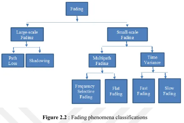
Figure 2.2 is showing the fading phenomena with its subcategories. The fading phenomenon can be classified in two types: one is large scale fading and the second is small scale fading.
Large scale fading occurs as the waves go through a large distance like the distance of the order of cell size [25]. As the signal is passing through a a long distance, the energy of the wave gets lower called path loss. Shadowing is a median path loss process caused by large objects such as buildings and vegetation. Small scale fading refers to rapid variation of signal levels in short distances.
Taking a brief look at propagated signal it is seen that[26]:
s(t) = Re{𝑠̃(t)𝑒𝑗2𝜋𝑓𝑐𝑡} (2.1)
r(t) = Re{∑𝑁 𝑐𝑛𝑒𝑗2𝜋(𝑓𝑐+𝑓𝐷,𝑛)(𝑡−𝜏𝑛)
11
Figure 2.2 : Fading phenomena classifications
here s(t) is the transmitted signal and 𝑠̃(t) is the equivalent signal in base band. Fc is
the carrier frequency, r(t) is the received signal after being effected by the channel and 𝑟̃(t) is the equivalent signal in base band. τn is delay and fD,n is the Doppler effect.
𝑟̃(t) = ∑𝑁 𝑐𝑛𝑒𝑗2𝜋𝜑𝑛(𝑡)
𝑛=1 𝑠̃(t - τn) (2.3)
𝜑𝑛(𝑡) = 2π(𝑓𝐷,𝑛𝑡 − (𝑓𝑐 + 𝑓𝐷,𝑛)𝜏𝑛 (2.4) 𝜑𝑛(𝑡) has a minus sign as fc is a large number.
This channel is a linear and time variant channel, which can be shown as:
𝑠̃(t) 𝑟̃(t) (2.5)
𝑠̃(t-τ) r’(t) ≠ 𝑟̃(t-τ) (2.6)
Because of existence of 𝑐𝑛𝑒𝑗𝜑𝑛(𝑡) part. Figure 2.3 shows a baseband transmission channel briefly.
12 g(t,τ) = ∑𝑁 𝑐𝑛𝑒𝑗𝜑𝑛(𝑡) 𝑛=1 δ(t- τn) (2.7) 𝑠̃(t) = a(t) 𝑒𝑗𝜃(𝑡) (2.8) r(t) = ∑𝑁𝑛=1𝑐𝑛Re{𝑒𝑗2𝜋(𝑓𝑐+𝑓𝐷,𝑛)(𝑡−𝜏𝑛) a(t- τn) 𝑒𝑗𝜃(𝑡−𝜏𝑛) } = ∑𝑁 𝑐𝑛a(t − 𝜏𝑛) 𝑛=1 cos [2𝜋(𝑓𝑐 + 𝑓𝐷,𝑛)(𝑡 − 𝜏𝑛) + 𝜃(𝑡 − 𝜏𝑛)] (2.9) 𝑠(𝑡) = 𝑎(𝑡)𝑐𝑜𝑠(2𝜋𝑓𝑐𝑡 + 𝜃(𝑡)) (2.10)
Depending on the relative extent of a multipath, frequency selectivity of a channel. is characterized (e.g., by frequency-selective or frequency flat) for small-scaling fading. Meanwhile, depending on the time variation in a channel due to mobile. speed (characterized by the Doppler spread), short- term fading can be classified as either fast fading or slow fading [27]. Figure 2.4 classifies the types of fading channels.Figure 3.4 show these types on the signal.
Figure 2.4 : Channel effects in wireless channels 2.1 Large-sclae Fading
Line of sight (LOS) environment is the channel when there is no obstacle between the transmitter and reciever. Satellite communication systems are LOS environments that are modeled with free space propagation forms. Showing the distance between the transmitter and reciever by d, the received power in free space environment using Friis equation [26] can be modeled as below:
Let d denote the distance in meters between the transmitter and receiver. When non-isotropic antennas are used with a transmit gain of Gt and a receive gain of Gr, the
received power at distance d, Pr(d), is expressed by the well-known Friis equation
13 Pr(d) = 𝑃𝑡𝐺𝑡𝐺𝑟𝜆
2
(4𝜋)2𝑑2𝐿 (2.11) where Pt is the transmit power in watts, Gt is the transmit gain and Gr is the reciever
gain of non-isotropic antennas, λ is the wavelength of radiation in meters and L is the system loss factor. System loss factor is completely independent of propagation environment and it represents the overall loss in the system hardware. In general, L is bigger than 1, but L cane be cosnsiderd to be equal to 1 if we assume that there is no loss in the system hardware. Considering the 2.1 formula, it is obviousthat the received power attenuates exponentially by the distance. Assuming that the system loss factor is equal to one,the free space path loss can be derived from Equation (2.6) as below:
PLf (d)[dB] = 10log(𝑃𝑡
𝑃𝑟) = -10 log(
𝐺𝑡𝐺𝑟𝜆2
(4𝜋)2𝑑2) (2.12) Without considering antenna gains, the equation 2.12 reduces to the equation below: PLf (d)[dB] = 10log(𝑃𝑡
𝑃𝑟) = 20 log(
4𝜋𝑑
𝜆 ) (2.13)
Figure 2.5 shows the free space path loss for different antenna gains whith carrier frequency equal to 1.5 GHz as the distance varies.
Figure 2.5 : Free space path loss model with fc = 1.5 GHz
Ita can be seen from figure 2.5 that the path loss is more less when the transmitter and receiever antenna gains are higher. By reducing the antenna gain of the reciever, free space path loss gets higher and even more, by reducing both receiving and
14
transmitting antennas, the pass loth gets considerably more higher. It was obvious that the average received signal decrease in a logarithmic manner by distance.
More general free space path loss model can be constructed by modifying the 2.13 formula with a path loss exponent that varies with the environment. This path loss environment is caleed log distance path loss model and is formulated as below: PLLD(d)[dB] = PLF(d0) + 10nlog(𝑑
𝑑0) (2.14)
Where n is the path loss exponent varied by different environments, d is the distance between the transmitter and the reciever and d0 is a reference distance . The path loss
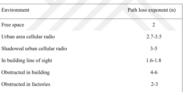
exponents is range from 2 to 6 depending on the propogation environment and shown in table 2.1. For the most basic environment ,free space, path loss wxponent is equal to 2 and in the complex invironments in urban areas obstructed with building it range fron 4 to 6. Full list is as below [34]:
Table 2.1 : Path loss exponent values for different environments
Environment Path loss exponent (n) Free space 2
Urban area cellular radio 2.7-3.5 Shadowed urban cellular radio 3-5 In building line of sight 1.6-1.8 Obstructed in building 4-6 Obstructed in factories 2-3
The other parameter, reference distance, should be determined properly for different environments also. This parameter is set as 1 Km for a cellular system with a cell radius greater than 10 Km. For Macro cellular systems with a cell radius of 1 Km, reference distance is considered as 100m and in micro cellular systems with smaller cell radius, this parameter is considered to be 1m.
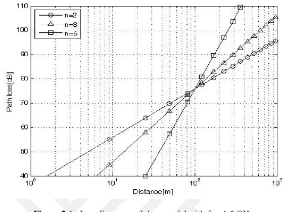
Figure 2.6 shows the log distance path loss with different path loss exponents and carrier frequency equal to 1.5 GHz.
15
Figure 2.6 : Log-distance path loss model with fc = 1.5 GHz
It is clear that the path loss increases with the path loss exponent n. Even if the distance between the transmitter and receiver is equal to each other, every path may have different path loss since the surrounding environments may vary with the location of the receiver in practice. However, all the aforementioned path loss models do not take this particular situation into account. A log-normal shadowing model is useful when dealing with a more realistic situation. Let Xs denote a Gaussian random
variable with a zero mean and a standard deviation of s [34]. Then, the log-normal shadowing model is given as
PL(d)[dB] = 𝑃𝐿̅̅̅̅(d)+X𝝈 = PLf(d0) + 10nlog(𝑑
𝑑0) +X𝝈 (2.15)
This modela is some how more realistic as it considers a Gaussian random variable with zero meand and standrad deviation of 𝝈 as the shadowning effect.
Figure 2.7 shows the log-normal shadowing model with path loss exponent equal to 2, standard deviation equal to 3 dB and carrier freauency equal to 1.5 GHz in three different random path models.
16
Figure 2.7 : Log-normal Shadowing path loss model with fc = 1.5 GHz
Some of more specific large scale channel models in literature are Okumara/Hata model, Cost-231 and Walfisch/Bernoti Model. [25],[34]:
2.1.1 Okumara/Hata model
Okumura model is one of the most frequently used path loss models that is obtained thhrough extensive computations of antenna height and coverage are experimentally in urban areas. This model covers the wireless communication models with frequency band of 500 MHz up to 1500 MHz, cell radius from 1km to 100 km and antenna heigh of 30 m up to 1 km.
Okumura equation is as below:
PLOK(d)[dB] = PLF + AMU(f,d) – GRx – GTx + GAREA (2.16)
where d is the distance between transmitter and the reciever, AMU(f,d) is the medium
attenuation factor at frequency f and distance d, GRx is the reciever antenna gain, GTx
is the transmitter antenna gain and GAREA is the the propagation environment gain in
specific areas. Antenna gains are a function of height of these antennas and antenna patterns are not taken into account. Meanwhile, AMU(f,d) and GAREA can be referred
17
to the graphs obtained by Okumura measurements in real experiences [27].
Hata model is only an extension of Okumura model including open, suburban and urban areas.
Hata model for urban areas equation is as below:
PLHATA,U(d)[dB] = 69.55 + 26.16 log fc -13.82loghTx – CRx +
(44.9 - 6.55 log hTx) log d (2.17)
Where hTx is the height of transmitter antenna , is the carrier frequency, d is the
distance between transmitter and reciever, CRx is the correlation coefficient of the
receiver antenna.
CRx can be calsulated as below in small to medium sized cell coverage areas:
CRx = 0.8 + (1.1 log fc – 0.7)hRx – 1.56 log fc (2.18)
where hRx is the height of transmitter antenna.
CRx can be calculated as below depending on the range of the carrier frequency in
large cell size areas:
CRx = {8.29 (log(1.54 ℎ𝑅𝑥))
2− 1.1 𝑖𝑓 150 𝑀𝐻𝑧 ≤ 𝑓
𝑐 ≤ 200 𝑀𝐻𝑧
3.2 (log(11.75 ℎ𝑅𝑥))2− 4.97 𝑖𝑓 200 𝑀𝐻𝑧 ≤ 𝑓𝑐 ≤ 1500 𝑀𝐻𝑧
(2.19) Hata model in suburban and open areas can be shown as below:
PLHata,SU(d)[dB] = PLHata,U(d)-2(log𝑓𝑐 28)
2 – 5.4 (2.20)
PLHata,O(d)[dB] = PLHata,U(d) - 4.78(logfc)2 – 18.33 log fc – 40.97 (2.21)
Figure 2.8 represents the path loss in urban, suburban and open areas. 2.1.2 COST 231 model
Cost 231 is and extention of Hata envoironment model to 2 GHz [34]. This extetion is done by European cooperative for scientific and technocal research (EUROCOST) and equation isas below:
Lurban(dB) = 46.3 + 33.9 log fc − 13.82 log (ht) − a(hr) + (44.9 − 6.55 log ht )* log d
+CM (2.22)
where a(hr) can be calculated as below:
18
Figure 2.8 : Hata path loss model with fc = 1.5 GHz
(2.23) a(hr) = (3.2 log 11.75 hr)2 – 4.97 dB for large cities (2.24)
CM can be determined as below:
CM = 0 dB for small to medium cities (2.25)
CM = 3 dB for large cities (2.26)
This model is caleed COST 231 in literature and has some restriction for carrier frequncy, distance and heght of transmitter and reciever. Carrier frequency in this model should be between 1.5 GHz and 2 GHz, transmitter height be between 30 and 200 meters, reciever height be between 30 and 200 meters and distance between 1 and 20 Km.
2.1.3 Walfisch/Bernoti model
COST 231 does not consider the impact of diffraction [34].Walfisch and Bernoti has introduced a model that predict average signal level at the street by using diffraction.
19
In this environment model, path loss is considered to be product of three factors as below:
L=P0Q2P1 (2.27)
where P0 is the omnidirectional antennas free space path loss, Q2 is the signal power
reduction because of buildings that block the receiver at street level, and P1 is the
signal power loss because of diffraction from the rooftop to the street level. 2.2 Small Scale Fading
small-scale fading is often referred to as fading in short. Fading is the rapid variation of the received signal level in the short term as the user terminal moves a short distance. It is due to the effect of multiple signal paths, which cause interference when they arrive subsequently in the receive antenna with varying phases. In other words, the variation of the received signal level depends on the relationships of the relative phases among the number of signals reflected from the local scatters. Furthermore, each of the multiple signal paths may undergo changes that depend on the speeds of the mobile station and surrounding objects. In summary, small-scale fading is attributed to multi-path propagation, mobile speed, speed of surrounding objects, and transmission bandwidth of signal.
2.2.1 Flat fading
Lets assume that τMax is maximum difference between delays of signals and defined
as below:
τMax = Max{ τi – τj } for every i,j (2.28)
Flat fading can be shown in an other way also: If Bc >> Bs , then the channel is flat fading channel.
Bc is coherence bandwidth and Bc = 1
𝜏𝑀𝑎𝑥 and Bs is the signal bandwidth and is defined as Bs = 1
𝑇𝑠 where Ts is symbol period.
Now we consider thet τi ≅ τj for every i and j
So τMax = 0 and in all time periods. We define τi ≅ τj ≅ 𝜏̂
So from equation (3.5) we have:
20 by taking furrier transform from both sides :
Fτ{g(t,τ)} = ∫−∞+∞𝑔(𝑡, τ)𝑒−𝑗2𝜋𝑓𝜏 dτ = ∫−∞+∞g(t) δ(t − τ𝑛)𝑒−𝑗2𝜋𝑓𝜏 dτ = g(t) 𝑒−𝑗2𝜋𝑓𝜏̂ =
T(t,f) (2.30)
|T(t,f)| = |g(t)| which means that for every frequency, in a time like t=t1 channel makes
the same effect on the signal.
The baseband equivalent of the received signal from equation (2.3) is as below: 𝑟̃(t) = ∑𝑁 𝑐𝑛𝑒𝑗𝜑𝑛(𝑡)
𝑛=1 𝑠̃(t - τn)= ∑𝑁𝑛=1𝑐𝑛𝑒𝑗𝜑𝑛(𝑡)𝑠̃(t - 𝜏̂) = g(t) 𝑠̃(t - 𝜏̂) (2.31)
This demonstrates that when the fading is flat , the signal is being multiplied by a fading factor named g(t) which is define as below:
g(t) = ∑𝑁 𝑐𝑛𝑒𝑗𝜑𝑛(𝑡)
𝑛=1 = ∑𝑁𝑛=1𝑐𝑛𝑐𝑜𝑠𝜑𝑛(𝑡) + j ∑𝑁𝑛=1𝑐𝑛𝑠𝑖𝑛𝜑𝑛(𝑡) = gI(t) + jgQ(t)
(2.32) the fading variables envelope and phase distribution as:
g(t) = gI(t) + j gQ(t) = ρ(t)𝑒𝑗𝜑(𝑡) (2.33)
ρ(t) = |g(t)| = √𝑔2
𝐼(𝑡) + 𝑔2𝑄(𝑡) (2.34)
𝜑(𝑡) = Arctan 𝑔𝑄(𝑡)
𝑔𝐼(𝑡) (2.35)
In flat fading channels, the effect of the channel is the same for all frequency ranges of the signal passing through the channel.
2.2.2 Frequency selective fading
In a frequency selective multipath fading channel ,in a fixed time such as t=t1, signal
is being effected by different powers. This happens when τMax ≅ Ts OR τMax > Ts
in other words, Bc ≤ Bs . The effect of this fading channel is in frequency domain
signal gets narrower and in time domain gets wider which causes inter symbol interference. In frequency selective channels, there are different channel effects on different frequencies of the signal passing through the channel.
2.3 Well Known Fading Channels
21
distribution in celllar networks. Even though Rayleigh fading can be achieved from Nakagami-m fading distribution, but this distribution worth studying. Rayleigh fading is known for its complexity in channel charachteristics.
2.3.1 Rayleigh fading
In Rayleigh fading there is no line of sight route between transmitter and receiver. gI(t)
and gQ(t) have Normal distribution with mean zero and variance 𝝈2 which is a different
amount for each. This means that variance of Normal distribution for gI(t) is different
than gQ(t). But we take the both variances the same which works true in practical
expriences. ρ𝑔𝐼𝑔𝑄 = 1
2𝜋𝜎2 𝑒
−𝑥2+𝑦2
2𝜎2 (2.36)
And pdf of this distribution is :
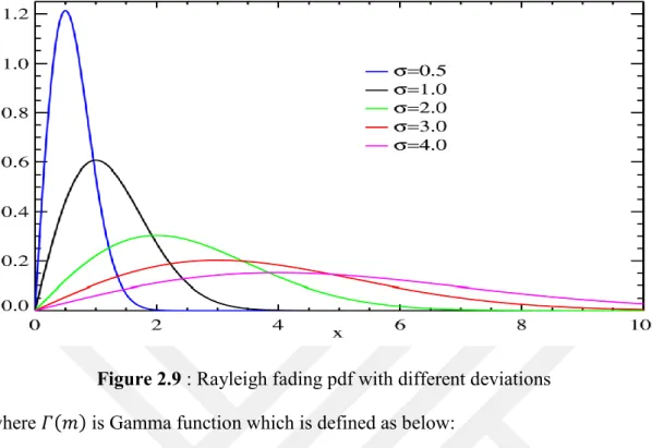
Pρ(x) = { 𝑥 𝜎2𝑒 −𝑥2 2𝜎2 𝑥≥0 0 𝑜𝑡ℎ𝑒𝑟𝑤𝑖𝑠𝑒 (2.37) φ(t) = arctan𝑔𝑄(𝑡) 𝑔𝐼(𝑡) (2.38)
φ(t) is a uniform distribution between –π and +π.
Figure 2.9 is the scheme of probability density function (PDF) of Rayleigh distribution with deviations equal to 0.5, 1, 2, 3 and 4 [35].
Amplitude = 𝑒− 1 2 𝜎 (2.39) E[ρ] = ∫ 𝜌𝑃𝜌(ρ)dρ = √ 𝜋 2.𝜎 (2.40) 𝝮 = E[ρ2]= 2𝝈2 (2.41) Variance = E[ρ2] – E2[ρ] = (2 - 𝜋 2) 𝝈 2 (2.42) 2.3.2 Nakagami-m fading
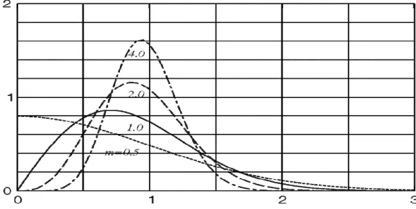
Nakagami-m fading is mostly being used for cellular communication and indoor and office channels. The pdf of the envelope is:
Pρ(x) = 2𝑚
𝑚𝑥2𝑚−1
𝛤(𝑚)𝛺𝑚 𝑒
−𝑚𝑥2𝛺 m≥1
22
Figure 2.9 : Rayleigh fading pdf with different deviations where 𝛤(𝑚) is Gamma function which is defined as below:
𝛤(𝑚) = ∫ 𝑦0∞ 𝑚−1𝑒−𝑦𝑑𝑦 m>0 (2.44) Figure 2.10 shows Nakagami-m distribution PDF with m values equal to 0.5, 1, 2 and 4.
Different m values makes the channel to be different known distributions. As the m value gets higher, channel gets more simple.
{m = 1 then it becomes a Rayleigh fading channel
m → ∞ then it gets similar to an AWGN fading channel (2.46) and showing the channel with Nakagami-m distribution has some advantages such as:
1. There is Bessel function which makes the analysis more easy
2. Has a very good approach to Rician channel which is the same as Rayleigh channel except there is a route of line of sight with the transmitter.
23
25
3. SYSTEM MODEL AND SPECTRUM SENSING ALGORITHMS
Let rd(t) be the continious signal that is received to the detector in the secondary user.
This signal can be shown as follow:
rd(t) = sd(t) + ηd(t) (3.1)
where sd(t) is the primary user’s signal and ηd(t) be the noise. Noise is assumed to be
a stationary process which satisfies the equations below:
E(ηd(t)) = 0 (3.2)
E(η2
d(t)) = 𝝈η2 (3.3)
E(ηd(t)ηd(t+τ)) = 0, for any τ≠0 (3.4)
In secondary users detectors, we are intrested in in the frequencies centered in fc and
the bandwidth be W. Detector get the samples of received signal with the sampling rate equal to fs which is bigger or equal to the bandwidth.
For simplifying the notations, we use the equations below:
x(n) = xd(nTs) (3.5)
s(n) = sd(nTs) (3.6)
η(n) = ηd(nTs) (3.7)
where Ts is the sampling period of the detector and equal to (fs)-1.
Spectrum sensing in the cognitive radio systems is a binary hypothesiscan be shown as follow [36]:
H0 : The spectrum band is in idle status (3.8)
H1 : The spectrum band is in busy status (3.9)
Received signals to detector under both hypothesis is given as:
26
H1 : x(n) = Hs(n) + η(n) (3.11)
where H is the effects of channel and η(n) is the is the white noise received which is assumed to be independent and identically distributed (iid) with mean equal to 0 and variance equal to 𝝈η2.
In multiple input multiple output systems, the received signal can be shown as below[23],[38]:
xi(n) = ∑𝑗=1𝑃 ∑𝑘=0𝑁𝑖𝑗 ℎ𝑖𝑗𝑠𝑗(𝑛 − 𝑘) + η𝑖(𝑛) (3.12)
where P is the number of signals in transmitter side, hij(k) is effect of the channel wich
is the channel response from source signal j to the antenna i and Nij is the order of
channel hij(k). The term h is the gain of the channel that effects the sent signal by the
primary user is mostly modeled as Nakahami-m fading channels in cell sized and indoor environments. Nakagami-m fading channel can mathematically modeled below: Pϼ = 2𝑚 𝑚𝑥2𝑚−1 Γ(m)Ω𝑚 exp(- 𝑚𝑥2 Ω ) , m ≥ 1 2 , x ≥ 0 (3.13) Γ(m) = ∫ 𝑦∞ 𝑚−1 0 𝑒 −𝑦𝑑𝑦 , 𝑚 > 0 (3.14)
where Γ(.) is a gamma function where Γ(1) is equal to 1. 3.1 Energy Detetion Based Spectrum Seninge Algorithms.
Energy detection is based on collecting received signals samples after prefiltering which limits the noise bandwidth and normalizes the noise variance. Afte accumulating these energy smaples of primary user, a comparison is being done. classical energy detection method and double threshold energy detection based spectrum sensings are the most well known spectrum sensing methods in this concept. 3.1.1 Classical energy detection:
An analog energy detector consists of a pre-filter, square law device and a finite time integrator. The output of the integrator is the normalized received signal energy of the receiver or detector. The normalized received signal energy is as follow [8]:
℮(t) = 1
𝑁∑ |𝑦(𝑛)| 2 𝑁−1
𝑛=0 (3.15)
Number of collected samples by detector is considered to be equal to N. Samples can be treated as a random process as the received signals are unknown. the sample
27
transmitted signals follows an independent and identically distributed (i.i.d) random processes with zero mean and variance of σ𝑠2. So that the received signal SNR in a
channel with gain of h can be shown as α=|ℎ|2𝜎𝑠2
𝜎𝜂2 . In the case that collected signals are large enough, using CLT, under hypothesis H0 , the probability density function (PDF)
of ℮(t) becomes a normal distribution with mean = N𝜎𝜂2and variance = N𝜎
𝜂4. The PDF
of ℮(t) , under hypothesis H1 , it is a normal distribution with mean = N(1+α)𝜎𝜂2 and
variance = (1+2α)N𝜎𝜂4. Considering the distributions above, the probability of false
alarm (Pfa) and probability of detection (Pd) can be shown as[36] :
Pfa = prob(℮(Ns)> λ|H0) = Γ(u,λ 2)/ Γ(u) = Q( λ− ση2 √2ση4/𝑁 ) (3.16) Pd= prob(℮(Ns)> λ|H1) = Qu(√2𝛼, √λ) = Q(λ− (|ℎ| 2𝜎 𝑠2+ση2) √2(|ℎ|2𝜎𝑠2+ση2)/N ) (3.17)
Where Q(.) is the Q-function. In the IEEE802.22 ,Pfa is equal to 0.1 as minimum but
generally for any Pfa we can calculate threshold based on Pfa as follow:
λfa = 𝝈η2 (1+ √2𝑄
−1(𝑝 𝑓𝑎)
√𝑁 ) (3.18)
In the case of hypothesis H1 , we can calculate the threshold based on Pd for any signal
to noise ratio (α) as follow: λd = 𝝈η2 (1+α)(1+ √2𝑄
−1(𝑝 𝑑)
√𝑁 ) (3.19)
In ED based spectrum sensing method the threshold calculated based on Pfa is
compared with the received signal to detect if the primary user is using the spectrum allocated or not. If the energy is bigger than the found threshold, the detector concludes the presence of the signal and absence in other case. Algorithm 3.1 shows the sensing procedure of energy detector.
Algorithm 3.1 : Energy Detection Based Spectrum Sensing Algorithm Input : λ, 𝝈η
Output : Ri
28 2: ℮(t) Energy of the N samples 3: if ℮(t) > λ then 4: Ri H1 5: else 6: Ri H0 7: return Ri 8: end for
ED sensing method is a semi blind spectrum sensing method. It is called semi blind because for measuring the threshold, instead of the Pfa, it needs the variance of noise
also. Measuring the exact variance of noise is not possible mainly and there could be some error in the calculation. Assume that ζ dB is the error accrued in noise estimation. θ = 10ζ/10 is the power of the error so that P
fa and Pd can be calculated as:
Pfa = prob(T(Ns)> λ|H0) = Γ(u,𝜃λ
2)/ Γ(u) (3.20)
Pd= prob(T(Ns)> λ|H1) = Qu(√2𝛼, 𝜃√λ) (3.21)
The biggest issue with ED spectrum sensing method in large cellular areas is the noise uncertainty. As this method, instead of Pfa, depends on the noise variance also,
measurement error in nise effects the performance of this method. Later, the effects of the noise uncertainty (NU) is going to be shown by simulations also.
A Monte-Carlo simulation model is developed in MATLAB software with i.i.d noise samples with Gaussian distribution and QPSK modulated random primary signals are used mentioned otherwise. It is assumed that the channel is stable and does not change during the period of sampling. To calculate the sensing threshold, only the noise variance and Pfa is needed for ED spectrum sensing algorithm. The probability of false
alarm is Pfa ≤ 0.1and probability of detection is Pd > 0.9 as required by IEEE 802.22
standard. Pfa is chosen equal to 0.1 in all of the simulations and results are avaraged
over 104 tests.
Figure 1 shows the performance of ED in different modulations such as BPSK, QPSK and 8PSK modulation types. Different modulation types is not affecting the performance of the detection method. This can be easiy seen from the this figure also
29
that modulation type does not effect the performance of the Energy detection based spectrum sensing.
Figure 2 shows the performance of ED sensing method with different signal types. Signals can be sent with different shapes. In this figure, different signal shapes are used such as rectangular, raised cosine and root raised cosine shapes. For abtaining such signal shapes, filters are used before sending it. This is obvious that the signal type is not effecting the sensing performance also.
Figure 3.1 : Energy Detection based spectrum sensing performance comparison with BPSK, QPSK and 8 PSK modulations.
As mentioned earlier as the m goes to infinity the channels distribution function gets nearer to Gaussian channel and if the m=1, the Nakagami-m channels gets the same distribution function as Rayleigh fading channel. The Gaussian channel has the best performance and Rayleigh fading has the worst performance among Nakagami-m fading channels.
There are different channel conditions in wireless channels as discussed before. Figure 3.3 shows the performance of ED sensing in different channels.
30
Figure 3.2 : Energy Detection based spectrum sensing performance comparison with different signal types such as rectangular, raised cosine and root raised cosine types.
Figure 3.3: Energy Detection sensing method performance of QPSK in Gaussian, Rayleigh and Nakagami-m fading channels with m=1, 2 and 15.
31
Figure 3.4. : Energy Detection based spectrum sensing method’s performance with 0, 0.5, 1, 1.5 and 2dB noise uncertainty for signal passing through Gaussian channel.
Figure 3.5. : Energy detection based spectrum sensing method performance with 0, 0.5, 1, 1.5 and 2dB noise uncertainty for signal passing through Rayleigh channel. Figure 3.4 shows the performance of ED sensing method in Gaussian channel and figure 3.5 show the performance of it in Rayleigh channel, both with nthe oise uncertainty of 0, 0.5, 1, 1.5 and 2dBs.
32
3.1.2 Double threshold energy detection based spectrum sensing method
Double threshold energy detection (DTED) spectrum sensing method is introduced to make ED sensing method more reliable. The main purpose in this method is to define a restricted area near to the threshold that the samples with small errors could be assemble in this area and do not affect the whole detection procedure. So, a restricted area constant (RAC) is chosen like θ to define the boundries of the restricted area as follow [40].
λ1 = (1-θ) λ for lower boundary (3.22)
λ2 = (1+θ) λ for higher boundary (3.23)
any value between or equal to these thresholds are not going to have any effect on the decision procedure. Algorith 3.2 shows the detection process of DTED method [36],[40].
Algorithm 3.2. : Double threshold energy detection based spectrum sensing method Input : θ, λ, 𝝈η
Output : Ri
1: for each sensing period do 2: ℮(t) Energy of the N samples 3: λ1 = (1-θ) λ 4: λ2 = (1+θ) λ 5: if ℮(t) < λ1 then 6: Ri H0 7: return Ri 8: else if ℮(t) > λ2 9: Ri H1 10: return Ri 11: else 12: return nothing 13: end for
33
In this method, instead of Pfa and Pd, two new probabilities can be defined as the
probability of the energy be between boundaries in condition of hypothesis H0 and H1
that can be shown as follow. Pfa = p(E(Ns)> λ2|H0) = Γ(u,λ2 2)/ Γ(u) (3.24) Pd= p(E(Ns)> λ2|H1) = Qu(√2𝛼, √λ2) (3.25) P0 = p(λ1<E(Ns)<λ2|H0) = (Γ(u,λ1 2)/ Γ(u)) – (Γ(u, λ2 2)/ Γ(u)) (3.26) P1=p(λ1<E(Ns)<λ2|H1)=Qu(√2𝛼, √λ1)-Qu(√2𝛼, √λ2) (3.27)
Detection performance of DTED gets low suddenly in low SNRs. This is because the percent of the samples containing information for detection process in RAC region gets high and effects the performance [21].
The Monte-Carlo simulation model developed in MATLAB for this section needs the noise variance, Pfa and RAC as well. Like previous section, Pfa is chosen as 0.1 in the
simulations and results are averaged over 104 tests, RACs are 0.025, 0.5, 0.75 and
noise variances are 1 and 2 dBs.
Figure 3.6 shows how many percent of the samples used in DTED, which are not in the restricted area with RAC of 0.5 in different channels. The number of usable samples in decision decrease as SNR decreases but then the number of samples increases. Although the number of samples used for detection increase but the performance of DTED does not get better. The reason is in low SNRs the valuable data that effects the performance of DTED is very near the border of original threshold in ED method.
In Figure 3.7, it is shown that how many percent of valuable data is eliminated because of restriction gap, which could effect the performance.
Figure 3.8 shows the effect of RAC on the percentage of usable data in DTED method in Gaussian channel. By increasing RAC rate, the percent of data in the restricted area increases.
In figure 3.9 it is shown that how increasing the RAC effects the percent of valuable data eliminated because of restriction gap.
34
In figure 3.10 The performance of DTED method in different channels. In high SNRs, DTED method has a good performance in all channels, but as the SNR gets lower, the performance of DTED gets lower because of the reasons described above.
Figure 3.6 : Percentage of the energy samples used to make decision using double threshold energy detection method with RAC=0.5 in different channels.
Figure 3.7 : Percentage of the valuable energy samples eliminated using double threshold energy detection method with RAC=0.5 in different channels.
35
Figure 3.8 : Percentage of the energy samples used in double threshold energy detction method with RAC = 0.25,0.5 and 0.75 in Gaussian channel .
Figure 3.9 : Percentage of the valuable energy samples eliminated using double threshold energy detection method with RAC= 0.25, 0.5 and 0.75in Gaussian
36
Figure 3.10 : Double threshold energy detection method with RAC = 0.5 performance comparison in different channels.
Figure 3.11 : Double threshold energy detection method with RAC = 0.25, 0.5 and 0.75 and Noise Uncertainty = 0, 1 and 2 dBs performance comparison in Gaussian
37
In figure 3.11 , the effects of noise uncertainty on the performance of DTED method with RACs equal to 0.25, 0.5 and 0.75 is shown in low SNRs. In this figure the signal is passing through a Gaussian channel. In low SNRs, DTED is very effective to Noise uncertainty that makes its performance unreliable. Actually, it gets better for lower RACs.
3.2 Covariance Based Spectrum Sensing
The received signal to the reciever signal is as below:
xi(n) = ∑𝑃𝑗=1∑𝑁𝑘=0𝑖𝑗 ℎ𝑖𝑗𝑠𝑗(𝑛 − 𝑘) + η𝑖(𝑛) (3.28)
Nij is the order of channel hij(k) and we define Nj as the Maximum of Nij over i.
Zero-padding the hij(k) should have been done if it is necessary[38]. We can define the
parameters as below:
𝒙(𝑛) = [x1(n),x2(n),x3(n), … , xM(n)]T (3.29)
hj(n)= [h1j(n),h2j(n),h3j(n), … , hMj(n)]T (3.30)
𝛈(𝑛) = [η 1(n), η 2(n), η 3(n), … , η M(n)]T (3.31)
Using formula 3.29, 3.30 and 3.31in formula 3.28 we have: x(n) = ∑ ∑𝑁𝑗 𝒉𝑗𝑠𝑗(𝑛 − 𝑘) + 𝛈(𝑛)
𝑘=0 𝑃
𝑗=1 , n=0,1,… (3.32)
By using the smoothing factor L consecutive outputs: 𝒙 ̅(𝑛) = [xT(n),xT(n-1),xT(n-2), … , xT(n-L+1)]T (3.33) 𝛈̅(𝑛) = [η T(n), η T(n-1), η T(n-2), … , η T(n-L+1)]T (3.34) 𝒔̅(𝑛) = [s1(n), s1(n-1), s1(n-2), … , s1 (n - N1 – L + 1) , … , sp(n), sp(n-1), sp(n-2), … , sp (n – Np – L + 1)]T (3.35) 𝑁 = ∑𝑃𝑗=1 𝑁𝑗 (3.36)
Usig formula 3.33, 3.34 and 3.35 in equation 3.32 we have: 𝒙
̅(𝑛) = ∆𝒔̅(𝑛) + 𝛈̅(𝑛) (3.37)
where ∆ is a ML*(N+PL) matrix defined as below:
38 ∆j=[ 𝒉𝑗(0) … … 𝒉𝑗(𝑁𝑗) ⋯ 0 ⋮ ⋱ ⋮ 0 … . 𝒉𝑗(0) … . ⋯ 𝒉𝑗(𝑁𝑗) ] (3.39) ∆j is a ML*(Nj+L).
Statistical covariance matrices of the signals and noises are:
Rx = E(𝒙̅(𝑛)𝒙̅̅̅(𝑛) ) 𝑻 (3.40)
Rs = E(𝒔̅(𝑛)𝒔̅̅̅(𝑛) ) 𝑻 (3.41)
Rη = E(η̅(𝑛)η̅̅̅(𝑛) ) 𝑻 (3.42)
Easily this can be shown that [30]:
Rx = ∆Rs∆T + 𝝈η2 IML (3.43)
where 𝝈η2 is the variance of the noise, and IML is the identity matrix of order ML.
Considering to have one transmitter and one receiver, the signal hypothesis are given respectively:
H0 : x(n) = η(n) n=0,1,2,… (3.44)
H1 : x(n) = ∑𝑁𝑘=0 ℎ(𝑘)𝑠(𝑛 − 𝑘) + 𝜂 (𝑛) n=0,1,2,… (3.48)
Figure 3.12 : A model of wireless communication
In figure 3.12, s(n) is the transmitted signal samples, x(n) is the received signal saples, channel effect is consisting of path loss, multipath fading and time dispersion shown with h(k) called channel response .η(n) are independent and identically distributed (iid)
39
white noise samples with zero mean and 𝝈η2 variance. N is the order of the channel
[37].
The recieved signal is as follow:
x(n)=s(n) + η(n) (3.49)
which s(n) is the signal passed through the channel affected by both large scale and small scale fading.
Autocorrelation matrix of x(n) is defined as below:
Rxx = Rss + 𝝈η2I (3.50)
considerinf subsamples of L constructive received signals we have:
𝑥̅(𝑛) = [x(n),x(n-1),x(n-2), … , x(n-L+1)]T (3.51) 𝜂̅(𝑛) = [η(n), η (n-1), η (n-2), … , η (n-L+1)]T (3.52) 𝑠̅(𝑛) = [s(n), s (n-1), s (n-2), … , s (n-L+1)]T (3.53) So, in the case of H1:
𝑥̅(𝑛) = ∆𝑠̅(𝑛) + 𝜂̅(𝑛) (3.54)
where ∆ is a L*(N+L) matrix defined as :
∆=[
ℎ(0) … … ℎ(𝑁) ⋯ 0
⋮ ⋱ ⋮
0 … . ℎ(0) … . ⋯ ℎ(𝑁)
] (3.55)
There is no infinite signal samples in real life. So, we only have access to the sample covariancematrix rather than the statistical one.
For computing sample covariance matrix we have: Rx(Ns) = 1
𝑁𝑠
∑𝐿−2+𝑁𝑠𝑥̅(𝑛) 𝑥̅ 𝑇(𝑛)
𝑛=𝐿−1 (3.56)
where Ns is the number of samples that are collected.
By using the Rx(Ns) matrix, maximum and minimum eigen-value is calculated and
shown by λmin and λMax signs respectivley.
In the last step, the algorithm decides if ratio of maximum eigen-value to the minimum eigen-value is bigger than T1 or not. If the ratio is bigger than T1, the spectrum sensing


![Figure 2.9 is the scheme of probability density function (PDF) of Rayleigh distribution with deviations equal to 0.5, 1, 2, 3 and 4 [35]](https://thumb-eu.123doks.com/thumbv2/9libnet/4198993.65214/45.892.172.752.419.660/figure-scheme-probability-density-function-rayleigh-distribution-deviations.webp)