Shallow buried object detection using GPR

іш т

SSÄÜD 023ΐΠ br.'ÍCTlOíl

SHALLOW BURIED OBJECT DETECTION USING

GPR

A THESIS

SUBMITTED TO THE DEPARTMENT OF ELECTRICAL AND ELECTRONICS ENGINEERING

AND THE INSTITUTE OF ENGINEERING AND SCIENCES OF BILKENT UNIVERSITY

IN PARTIAL FULFILLMENT OF THE REQUIREMENTS FOR THE DEGREE OF

MASTER OF SCIENCE

By

Nejat Kamacı

August 1999

τ κ

-Κ36

I certify th at I have read this thesis and that in my opinion it is fully adequate, in scope and in quality, as a thesis for the degree of Master of Science.

Assist. Prof. Dr. Orhan Arikan(Sup(irvisor)

I certify that I have read this thesis and that in my opinion it is fully adequate, in scope and in quality, as a thesis for the degree of Master of Science.

Assoc. P ro r Dr. Levent Gürel

I certify that I have read this thesis and that in my opinion it is fully adequate, in scope and in quality, as a thesis for the degree of Master of Science.

Assoc. Hrof. Dr. Billur Barshan

Approved for the Institute of Engineering and Sciences:

< at

Prof. Dr. Mehrnetymray

Director of Institute of Engineering and Sciences

ABSTRACT

SHALLOW BURIED OBJECT DETECTION USING

GPR

Nejat Kamacı

M.S. in Electrical and Electronics Engineering

Supervisor: Assist. Prof. Dr. Orhan Arikan

August 1999

Ground Penetrating Radar received considerable attention in the use of shallow buried object detection. Differing from the traditional sensor systems such as electro magnetic induction based metal detector sensor, GPR can be used for objects with any property and any shape for a wide range of desired sensitivity and specificity. In this thesis, based on a simplified but robust measurement, model a three-stage algorithm is proposed for the real-time detection and lo­ calization of the shallow buried objects by using GPR measurements. Since all three stages of the proposed approach have environment adaptive features, the detection performance remains successful in a wide range of scenarios that can be encountered in applications.

Keywords: Ground Penetrating Radar, Background Removal, Adaptive Corre­

lation

ÖZET

GPR KULLANILARAK YÜZEYE YAKIN GÖMÜLÜ CİSİM

TESPİTİ

Nejat Kamacı

Elektrik ve Elektronik Mühendisliği Bölümü Yüksek Lisans

Tez Yöneticisi: Yrd. Doç. Dr. Orhan Arıkan

Ağustos 1999

Toprak Delici Radar son zamanlarda sığ gömülü cisimlerin tespitinde oldukça büyük ilgi toplamaktadır. Elektromanyetik endüksiyona dayalı metal tespitleyici duyucu gibi alışılagelmiş duyucuların tersine toprak delici radar her türlü şekilde ve büyüklükteki cismin geniş bir duyarlılık ve isterlerde tespitinde kullanılabilmektedir. Bu tezde, basitleştirilmiş ancak gürbüz bir ölçüm mod­ elinden yola çıkarak sığ gömülü cisimlerin toprak delici radar yardımıyla gerçek zamanlı tespiti ve yer kestirimini amaçlayan üç aşamalı bir algoritma sunulmak­ tadır. Sunulan algoritmanın her üç aşamasında da ortama uyarlama özellikleri olduğundan, uygulamalarda karşılaşılabilmesi muhtemel bir çok senaryoda tespit başarılı bir şekilde yapılabilmektedir.

Anahtar Kelimeler. Toprak Delici Radar, Ortam Çıkarımı, Uyarlamalı Kore­

lasyon

A C K N O W L E D G M E N T S

I would like to use this opportunity to express rny deep gratitude to my supervi­ sor Assist. Prof. Dr. Orhan Arikan for his guidance, suggestions and invaluable encouragement throughout the development of this thesis.

I would like to thank Assoc. Prof. Dr. Levent Gürel and Uğur Oğuz for their help and support. I would also like to thank Assoc. Prof. Dr. Levent Gürel and .\ssoc. Prof. Dr. Billur Barshan for reading and commenting on the thesis.

C ontents

1 INTRODUCTION 1

2 DETECTION OF BURIED OBJECTS BY USING GPR 4

2.1 Review of Literature on GPR Processing Techniques 8

3 PROPOSED APPROACH FOR THE DETECTION OF

BURIED OBJECTS BY USING GPR n

3.1 The first stage of processing of a GPR measurement 12

3.2 The second stage of processing of a GPR measurement 17

3.3 The third stage of processing of a GPR m ea su re m e n t... 26

3.4 Considerations In The Real-Time Application Of The Proposed A lg o rith m ... 27

4 RESULTS 29

4.1 Simulation Based R esults... 29

4.2 Laboratory Mcasureincnts ₄₈

5 CONCLUSIONS 68

List of Figures

2.1 Basic scheme of operation... 4

2.2 A sample one-dimensional A-scan... 5

2.3 A sample two-dimensional B-scan obtained by moving the GPR along a straight line passing over buried object. 5 2.4 Direct coupling (1), air-ground interface reflected (2) and object

scattered (3) signals... 6

3.1 The scheme of the proposed GPR processing approach for the detection of buried objects... 13

3.2 Example for the first stage of processing, (a) Acquired B-scan measurement, (b) Object scattered signal estimate obtained by the first stage of processing. 17

3.3 (a) Acquired raw B-scan measurement, (b) Object scattered signal estimate obtained by the first stage of processing. Depth dependent correlations (a) Ci, (b) C2, (cjCa and (d) C4 obtained

by the second stage of processing. 20

3.4 Normalized depth dependent correlations (a) NCi , (b) N C2,

(c) N C3 and (d) N C4 obtained by the second stage of processing. 23

3.5 Example; (a) Acquired raw B-scan measurement, (b) Object scattered signal estimate obtained by the first stage of pro­ cessing. Normalized depth dependent correlations (a) NCi, (b) NC'2, (c) N C3 and (d) NC,i obtained by the second stage

of processing, (g) Decision signal D2{x,y), dotted line is the

threshold, (h) Decision signal Di{x, y), dotted line is the thresh­

old. 25

4.1 GPR image obtained by simulation. The ground is modeled as homogeneous, and lossless. The object is a cylindrical plastic object with diameter = 5cm with relative dielectric constant e = 3. The ground dielectric constant is chosen to be e = 8. The top of the object is 8 cm below the surface, (a) Acquired raw B-scan measurement, (b) Object scattered signal estimate obtained by the first stage of processing. Normalized depth dependent correlations (a) NCi, (b) N C2, (c) N C3 and (d) N C4 obtained

by the second stage of processing, (g) Decision signal D2{x,y),

dotted line is the threshold, (h) Decision signal D4{x,y), dotted

line is the threshold. 33

3. The ground dielectric constant is chosen to be e = 8. The top of the object is 8 cm below the surface, (a) Acquired raw B-scan measurement, (b) Object scattered signal estimate obtained by the first stage of processing. Normalized depth dependent correlations (a) NCu (b) N C2, (c) N C3 and (d) obtained

by the second stage of processing, (g) Decision signal D2{x,y),

dotted line is the threshold, (h) Decision signal D^{x,y), dotted line is the threshold... 34 4.2 GPR image obtained by simulation. The ground is modeled as

heterogeneous, but lo,ssless. The object is a c}dindrical plastic object with diameter = 5cm with relative dielectric constant c =

4.3 GPR image obtained by simulation. The ground is modeled as heterogeneous, and lossy with a = 0.1 S/ m. The object is a plastic 5 x 5 x 4 prism with relative dielectric constant e = 3. The ground dielectric constant is chosen to be e = 8. The top of the object is 2 cm below the surface, (a) Acquired raw B-scan measurement, (b) Object scattered signal estimate obtained by the first stage of processing. Normalized depth dependent correlations (a) NC\, (b) N C2·, (c) NC^ and (d) NC^ obtained

by the second stage of processing, (g) Decision signal D2{x,y),

dotted line is the threshold, (h) Decision signal D^{x,y)i dotted

4.4 GPR image obtained by simulation. The ground is modeled as heterogeneous, and lossy with a = 0 . 1 S / m. The object is a plastic 5 x 5 x 4 prism with relative dielectric constant e = 3. The ground dielectric constant is chosen to be e = 8. The top of the object is 15 cm below the surface, (a) Acquired raw B-scan measurement, (b) Object scattered signal estimate obtained by the first stage of processing. Normalized depth dependent correlations (a) A^Ci, (b) N C2, (c) NCz and (d) NC\ obtained

by the second stage of processing, (g) Decision signal D2(a;, y), dotted line is the threshold, (h) Decision signal Di{x,y), dotted line is the threshold... ...36

4.5 GPR image obtained by simulation. The ground is modeled as heterogeneous, and lossy with a = 0.1 S / m. The object is a plastic 5 x 5 x 4 prism with relative dielectric constant e = 3. The ground dielectric constant is chosen to be e = 8. The top of the object is 8 cm below the surface, (a) Acquired raw B-scan measurement, (b) Object scattered signal estimate obtained by the first stage of processing. Normalized depth dependent correlations (a) NCi, (b) N C2, (c) NC^ and (d) N C4 obtained

by the second stage of processing, (g) Decision signal D2{x,y),

dotted line is the threshold, (h) Decision signal 1)4(0:, y), dotted

line is the threshold. 37

4.6 GPR image obtained by simulation. The ground is modeled as heterogeneous, and lossy with a =0. 15 S / m. The object is a plastic 5 x 5 x 4 prism with relative dielectric constant e = 3. The ground dielectric constant is chosen to be e = 8. The top of the object is 8 cm below the surface, (a) Acquired raw B-scan measurement, (b) Object scattered signal estimate obtained by the first stage of processing. Normalized depth dependent correlations (a) NCi, (b) N C2, (c) NC^ and (d) NC^ obtained

by the second stage of processing, (g) Decision signal £>2(2;, y), dotted line is the threshold, (h) Decision signal Di{x,y), dotted line is the threshold... 38

4.7 GPR image obtained by simulation. The ground is modeled as heterogeneous, and lossy with a = 0.2 S / m. The object is a plastic 5 x 5 x 4 prism with relative dielectric constant € = 3. The ground dielectric constant is chosen to be e = 8. The top of the object is 8 cm below the surface, (a) Acquired raw B-scan

I

measurement, (b) Object scattered signal estimate obtained by the first stage of processing. Normalized depth dependent correlations (a) NC\, (b) N C2, (c) NCs and (d) N C4 obtained

by the second stage of processing, (g) Decision signal D2{x,y),

dotted line is the threshold, (h) Decision signal £>4(2;, y), dotted

line is the threshold. 39

4.8 (a) The first model for the ground, (b) Top view. The ground has 20 holes at the surface level. In the medium depth level there are randomly placed 25 small lossy objects having cr = 0.1 — 0.2 and different relative dielectric constants. In the deeper depth level there are randomly placed 500 small lossy objects having

o = 0.03 — 0.04 and different relative dielectric constants. 40 4.9 (a) The fourth model for the ground, (b) Top view. The ground

has 40 holes at the surface level. In the medium depth level there are randorrdy placed 50 small lossy objects having cr = 0.1 — 0.2 and different relative dielectric constants. In the deeper depth level there are randomly placed 100 small lossy objects having

o — 0.03 — 0.04 and different relative dielectric constants. 41 4.10 (a) The third model for the ground, (b) Top view. The ground

has 60 holes at the surface level. In the medium depth level there are randomly placed 75 small lossy objects having <7 = 0.1 — 0.2 and different relative dielectric constants. In the deeper depth level there are randomly placed 150 small lossy objects having (j = 0.03 — 0.04 and different relative dielectric constants. 42

4.11 (a) The fourth model for the ground, (b) Top view. The ground has 80 holes at the surface level. In the medium depth level there are randomly placed 100 small lossy objects having a = 0.1 — 0.2 and different relative dielectric constants. In the deeper depth level there are randomly placed 200 small lossy objects having

o — 0.03 — 0.04 and different relative dielectric constants. 43

The ground dielectric constant is chosen to be e = 8. The top of the object is 8 cm below the surface, (a) Acquired raw B-scan measurement, (b) Object scattered signal estimate obtained by the first stage of processing. Normalized depth dependent correlations (a) NCi, (b) N C2, (c) NC-i and (d) obtained

by the second stage of processing, (g) Decision signal D2{x,y),

dotted line is the threshold, (h) Decision signal D^{x,y), dotted line is the th r e s h o ld ... 44 4.12 GPR image obtained by simulation. The ground is modeled as

given in Figure 4.8. The object is a cylindrical plastic object with diameter = 5cm with relative dielectric constant e = 3.

4.13 GPR image obtained by simulation. The ground is modeled as given in Figure 4.9. The object is a cylindrical plastic object with diameter = 5cm with relative dielectric constant e = 3. The ground dielectric constant is chosen to be e = 8. The top of the object is 8 cm below the surface, (a) Acquired raw B-scan measurement, (b) Object scattered signal estimate obtained by the first stage of processing. Normalized depth dependent correlations (a) NCi, (b) N C2·, (c) NCz and (d) NC^ obtained

by the second stage of processing, (g) Decision signal D2{x,y),

dotted line is the threshold, (h) Decision signal D^{x,y), dotted

line is the threshold. 45

The ground dielectric constant is chosen to be c = 8. The top of the object is 8 cm below the surface, (a) Acquired raw B-scan measurement, (b) Object scattered signal estimate obtained by the first stage of processing. Normalized depth dependent correlations (a) NCi, (b) NC-2, (c) NC'i and (d) NC/[ obtained

by the second stage of processing, (g) Decision signal D2{x,y),

dotted line is the threshold, (h) Decision signal D4{x,y), dotted

line is the threshold... ... 46 4.14 GPR image obtained by simulation. The ground is modeled as

given in Figure 4.10. The object is a cylindrical plastic object with diameter = 5cm with relative dielectric constant e = 3.

4.15 GPR image obtained by simulation. The ground is modeled as given in Figure 4.11. The object is a cylindrical plastic object with diameter = 5cm with relative dielectric constant e = 3. The ground dielectric constant is chosen to be e = 8. The top of the object is 8 cm below the surface, (a) Acquired raw B-scan

i

measurement, (b) Object scattered signal estimate obtained by the first stage of processing. Normalized depth dependent correlations (a) NCi, (b) NC^, (c) N C3 and (d) N C4 obtained

by the second stage of processing, (g) Decision signal D2{x,y),

dotted line is the threshold, (h) Decision signal D4{x,y), dotted

line is the threshold. 47

4.1G A piece of rock, buried at 2 cm depth. The ground is dry soil, (a) Acquired raw B-scan measurement, (b) Object scattered signal estimate obtained by the first stage of processing. Normalized depth dependent correlations (a) A’C'i, (b) N C2, (c) NCz and

(d) NCi obtained by the second stage of.processing. (g) Decision signal D2{x,y), dotted line is the threshold, (h) Decision signal

D4{x,y), dotted line is the threshold. 52

4.17 A piece of rock, buried at 5 cm depth. The ground is dry soil, (a) Acquired raw B-scan measurement, (b) Object scattered signal estimate obtained by the first stage of processing. Normalized depth dependent correlations (a) NCi, (b) N C2, (c) N C3 and

(d) NCi obtained by the second stage of processing, (g) Decision signal D2{x,y), dotted line is the threshold, (h) Decision signal

Di{x,y)·, dotted line is the threshold. 53 4.18 A piece of rock, buried at 15 cm depth. The ground is dry

soil, (a) Acquired raw B-scan measurement, (b) Object scat­ tered signal estimate obtained by the first stage of processing. Normalized depth dependent correlations (a) NC\ , (b) N C21

(c) NCz and (d) NCi obtained by the second stage of process­ ing. (g) Decision signal D2{x,y), dotted line is the threshold.

(h) Decision signal Di{x,y), dotted line is the threshold. 54

4.19 A piece of rock, buried at 2 crn depth. The ground is wet soil, (a) Acquired raw B-scaii measurement, (b) Object scattered signal estimate obtained by the first stage of processing. Normalized depth dependent correlations (a) NCi, (b) N C2, (c) N C3 and

(d) N C4 obtained by the second stage of processing, (g) Decision

signal D2(a;,y), dotted line is the threshold, (h) Decision signal

D^{x,y), dotted line is the threshold. 55 4.20 A piece of rock, buried at 2 cm depth. The ground is dry sand.

(a) Acquired raw B-scan measurement, (b) Object scattered sig­ nal estimate obtained by the first stage of processing. Normal­ ized depth dependent correlations (a) NCi , (b) NC^, (c) N C3

and (d) NCi obtained by the second stage of processing, (g) De­ cision signal D2{x,y), dotted line is the threshold, (h) Decision

signal Di{x,y), dotted line is the threshold. 56 4.21 A piece of rock, buried at 5 cm depth. The ground is dry sand.

(a) Acquired raw B-scan measurement, (b) Object scattered sig­ nal estimate obtained by the first stage of processing. Normal­ ized depth dependent correlations (a) NCi, (b) NC2, (c) NC3

and (d) NCi obtained by the second stage of processing, (g) De­ cision signal D2{x,y)·, dotted line is the threshold, (h) Decision

signal Di{x,y), dotted line is the threshold. 57

4.22 A piece of rock, buried at 15 cm depth. The ground is dry sand, (a) Acquired raw B-scan measurement, (b) Object scat­ tered signal estimate obtained by the first stage of processing. Normalized depth dependent correlations (a) A''C'i, (b) NC-z, (c) NC'i and (d) NC^ obtained by the second stage of process­ ing. (g) Decision signal Dzix.y), dotted line is the threshold. (h) Decision signal D^{x,y), dotted line is the threshold. 58 4.23 A piece of rock, buried at 2 cm depth. The ground is wet sand.

(a) Acquired raw B-scan measurement, (b) Object scattered sig­ nal estimate obtained by the first stage of processing. Normal­ ized depth dependent correlations (a) NCi , (b) NCz, (c) N C3

and (d) N C4 obtained by the second stage of processing, (g) De­

cision signal Dz{x,y), dotted line is the threshold, (h) Decision signal D4{x,y), dotted line is the threshold. 59

4.24 A coke can, buried at 2 cm depth. The ground is dry soil, (a) Acquired raw B-scan measurement, (b) Object scattered signal estimate obtained by the first stage of processing. Normalized depth dependent correlations (a) NCi, (b) NCz, (c) N C3 and

(d) N C4 obtained b)' the second stage of processing, (g) Decision

signal Dzix.y), dotted line is the threshold, (h) Decision signal

D4{x,y), dotted line is the threshold. 60

4.25 A coke can, buried at 5 cm depth. The ground is dry soil, (a) Acquired raw B-scan measurement, (b) Object scattered signal estimate obtained by the first stage of processing. Normalized depth dependent correlations (a) .VCi, (b) N C2, (c) NCj, and

(d) NC^ obtained by the second stage of processing, (g) Decision signal D2{x,y), dotted line is the threshold, (h) Decision signal

D4{x,y), dotted line is the threshold. 61

4.26 A coke can, buried at 15 cm depth. The ground is dry soil, (a) Acquired raw B-scan measurement, (b) Object scattered signal estimate obtained by the first stage of processing. Normalized depth dependent correlations (a) NCi, (b) N C2, (c) NCs and

(d) NCi obtained by the second stage of processing, (g) Decision signal D2{x,y), dotted line is the threshold, (h) Decision signal

Di{x,y), dotted line is the threshold. 62 4.27 A coke can, buried at 2 cm depth. The ground is wet soil, (a)

Acquired raw B-scan measunament. (b) Object scattered signal estimate obtained by the first stage of processing. Normalized depth dependent correlations (a) -VCi, (b) N C2, (c) N C2, and

(d) NCi obtained by the second stage of processing, (g) Decision signal D2{x,y), dotted line is the threshold, (h) Decision signal

Di{x,y), dotted line is the threshold. 63

4.28 A coke can, buried at 2 cm depth. Tlie ground is dry sand, (a) Acquired raw B-scan measurement, (b) Object scattered signal estimate obtained by the first stage of processing. Normalized depth dependent correlations (a) NC\_, (b) N C2, (c) NC-i and

(d) NC^ obtained by the second stage of processing, (g) Decision signal D2{x,y), dotted line is the threshold, (h) Decision signal

DA{x,y)·, dotted line is the threshold. 64 4.29 A coke can, buried at 5 cm depth. The ground is dry sand, (a)

Acquired raw B-scan measurement, (b) Object scattered signal estimate obtained by the first stage of processing. Normalized depth dependent correlations (a) NC\, (b) N C2, (c) NCs and

(d) N C4 obtained by the second stage of processing, (g) Decision

signal D2{x,y), dotted line is the threshold, (h) Decision signal

D\{x,y), dotted line is the threshold. 65 4.30 A coke can, buried at 15 cm depth. The ground is dry sand, (a)

Acquired 'raw B-scan measurement, (b) Object scattered signal estimate obtained by the first stage of processing. Normalized depth dependent correlations (a) NC\ , (b) N C2·, (c) NCz and

(d) NC\ obtained by the second stage of processing, (g) Decision signal D2{x,y), dotted line is the threshold, (h) Decision signal

D4{x,y), dotted line is the threshold. 66

4.31 A coke can, buried at 2 crri depth. The ground is wet sand, (a) Acquired raw B-scan measurement, (b) Object scattered signal estimate obtained by the first stage of processing. Normalized depth dependent correlations (a) NCi^ (b) N C2·, (c) A/'Qj and

(d) N Ca obtained by the second stage of processing, (g) Decision

signal D2{x,y), dotted line is the threshold, (h) Decision signal

DA{x,y), dotted line is the threshold. 67

Chapter 1

IN TR O D U C T IO N

Ground penetrating radar (GPR) is a recently developed sensor to detect and identify structures within the ground. GPR is by far the most advanced method of non-destructive and non-intrusive subsurface investigation. Traditional tech­ niques such as acoustic, electro magnetic inductive and electrical resistivity techniques do not offer the specificity and sensitivity offered by GPR. The benefits of this technique are based on its abilities to send continuous pulses while moving over the surface, and to change pulse frequencies as conditions dictate. This allows the technique to be customized for each unique situa­ tion [1-3,6,20].

Detection of buried objects has found wide application areas including rail­ way mapping, archaeology, environmental site assessment, forensics, glaciology, land mine and unexploded ordnance (UXO) detection, ground water studies, mining, rebar/conduit mapping, road and pavernent/concrete surveys, struc­ tural assessment, sewer mapping and utility detection [3,21]. Depending on the

specifications of the application the utilized sensors and the techniques show significant variations. Detection of deeper objects and structures requires the ability to penetrate deep into the earth which can be achieved by using seismic sources. There is a vast literature on results obtained by using seismic sensors and the detection algorithms. In this work, we are primarily interested in the detection of objects buried in the first few decimeters of the earth.

GPR became one of the most important sensor technology in shallow buried object detection. This is mainly because GPR can be used for detection of any kind of metallic and non-metallic objects. Especially in land mine and UXO Detection, GPR received so much attention because of its edge over induction based sensors in detecting objects with little or no metal content. Widespread deployment of anti-personnel plastic mines in many densely populated areas causes significant loss of life and maiming during the peace time. GPR allows a safer, quicker and cheaper choice. It is commonly used in the mine-clearance campaigns.

The data obtained by a GPR is rich enough to obtain high-resolution images of the subsurface structures. However, GPR has some limitations in operation. The depth of exploration and image definition is limited and depend on the radio frequency used. Low frequencies are used for deeper geological mapping. High frequencies are necessary for high-definition imaging, such as defect sur­ veys in concrete. In many areas, where both high resolution and penetration depth are needed, wider operation frequency bands are used, which yield ultra wide band (UWB) Radars.

In all cases, raw GPR measurements are hard to interpret, and requires sophisticated signal processing. Differing from the well-known “through the aii’'

radars, signal-to-clutter ratio is remarkably low. The air-ground interface is a major clutter source. Also, the changing ground properties (wetness, surface roughness, etc.) cause signiiicant deformation on the recorded signals than the transmitted one. Therefore traditional processing tools developed for detection of targets in clutter fail the detection of buried objects.

In most applications, GPR signal processing aims at the enhancement of the raw image scans, such that the relevant information becomes more prominent. Reliable detection is achieved by utilizing a matched filter on the processed image scans. As a requirement of some important applications, the size and the depth of the objects can also be estimated.

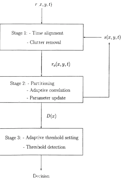
In this work, a robust, and computationally efficient processing technique will be presented. The proposed solution consists of three stages: adaptive clutter removal on each individually recorded signal, depth dependent adaptive matched filtering, and threshold detection.

In Chapter 2, the principle of operation of GPR will be described, and a model of the GPR measurement data will be introduced. Then, a short review of literature on GPR will be presented. In Chapter 3, the proposed approach for the detection of buried objects by using GPR will be presented. Starting with a simplification on the data model, the proposed three-stage processing approach will be detailed. In Chapter 4, the performance of the proposed approach is investigated by using both the actual and simulated GPR measurements. Finally, in Chapter 5 conclusions will be drawn.

Chapter 2

D ETEC TIO N OF B U R IE D

OBJECTS B Y U SIN G G P R

GPR is a sensor system basically composed of a radio transmitter and receiver, connected to a pair of directed antennas coupled to the ground. A typical operational scheme of a GPR is shown in Figure 2.1.

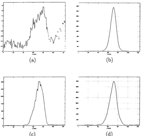
The transmitter generates electro magnetic pulses in the frequency range of 100-1000 MHz which are directed to penetrate into the ground by the trans­ mitter antenna. Anomalies in the local ground electro magnetic properties (relative dielectric constant or conductivity) due to foreign materials such as pipelines, cavities or land mines cause a scattering of the pulse. The receiving antenna is designed to capture the scattered field so that digitized samples of which are recorded for later processing. The recorded samples corresponding to a single pulse transmission is called an A-scan. Typically, the GPR is moved a small distance on a predetermined path to obtain successive A-scans and com­ bining these one dimensional informations form a two dimensional information which is called as a B-scan. In Figures 2.2 and 2.3 examples for both a one dimensional A-scan and two-dimensional B-scan are shown.

time (nsecs)

Figure 2.2: A sample one-dimensional A-scan.

60 80

X (c m )

100 120

Figure 2.3: A sample two-dimensional B-scan obtained by moving the GPR along a straight line passing over buried object.

The recorded signal mainly consists of three components: The first compo­ nent is the direct coupling signal from the transmitter to the receiver. Effective design methods such as pulse shaping, use of absorber and directive antennas help reduce the relative contribution of this component to the overall recorded signal at the receiver. The second component is the reflected signal from air- ground interface. The third and the final component is the object-scattered signal, which is the primary source of information for detection. In general, the contribution of the object scattered field is far less than the other contri­ butions to the recorded signal. Thus, the reflections from air-ground interface inherently reduce the performance of detection rates compared to those of commonly used radars operating through the air. In Figure 2.4 an example A-scan is shown to emphasize the relative strengths of the recorded signals. As seen from this figure the object scattered signal is received later in time. However, depending on the depth of the object and the pulse duration, the object-scattered signal may have significant overlap in time with the other signals.

Figure 2.4: Direct coupling (1), air-ground interface reflected (2) and object scattered (3) signals.

One single measurement of the GPR is not sufficient for processing and interpretation. This is because the measured signal does not match with the transmitted one, and the received signal characteristics may show significant variation depending on the ground pro])erties. Fortunately, the rich informa­ tion of a B-scan helps to resolve a lot of the difficulties associated with an A-scan.

In the rest of this section, we will provide a simple model for an A-scan which will be denoted as r{x,y,t), explicitly showing its dependence on the position of the GPR and time. For the purpose of detection, the recorded signal r{x, y, t) can be modeled as:

r{x,y,t) rc{x,y,t) . if there is no buried object (2.1)

Tcix, t/, t) + ro{x, y, t) . if there is a buried object.

where at each new position (x, y) of the GPR, time is restarted with the pulse transmission. In this expression, ro{x,y,t} represents the contribution in the received signal due to the scattered field of an object. Therefore, Tc(x, y, i) is the background clutter recorded at the receiver antenna. The purpose of detection is robust identification of the existence of a buried object by using a successive set of A-scans which is called as a B-scan. In the rest of this chapter, we will provide a short review on the available processing techniques.

2.1

R eview o f Literature on G P R P rocessin g

Techniques

Due to its widespread use in many important application areas, significant research effort has been spent to obtain better and more efficient techniques of detection for the GPR measurements. Here we provide a short review of the literature on the detection approaches developed for GPR. Several work on detection of shallow buried objects using GPR find place in the literature.

Perrig presents several methods and compares them for image enhancement in his work [19]. In the developed methods of image enhancement the utilized processing tools include: mean filtering, median filtering, background removal, horizontal line filter, Gaussian filter, ideal color representation, gradient flow diagram, restricted color representation and histogram equalization. For back­ ground removal, subtraction of the mean of a line of input pixels from each pixel on the same row is offered. Another method includes high-pass filtering to remove the horizontal lines on the raw B-scan image which are due to clutter. It is assumed that in the recorded B-scans, object images are in the shape of diffraction hyperbola. To improve the contrast of the image, histogram equal­ ization method is utilized. In order to do this, the intensities are re-mapped by applying a function which spreads the intensities that are close to the highest histogram value apart. A sigmoid transfer function of the form 2.2 is chosen as the suitable choice:

For the detection of objects on the enhanced images, methods based on Fourier transform analysis and neural networks are proposed. However, choosing the training set in this method creates a major problem.

In a study by Sheers, Pictte and Vander Vorst, after a standard average removal, filtering each A-scan with a Morlet wavelet filter is proposed [10]. De­ pending on the type of the object, the optimum central frequency, at which the object scatters maximum energy changes. They offer further tests and investi­ gations to be performed to determine which parameters influence the optimal central frequency of the filter. The need for adjustment of the parameters for different scenarios is a drawback of this method. Especially in real-time operations, this method is not practical to be used.

In another study by van Kempen, Sahli, Nyssen and Cornelis, removal of background clutter and measurement noise is attempted by adaptive filtering [12]. Among several filter types investigated in this work, the best performance is obtained with the use of the Wiener filter. They also offer time alignment and normalization for each A-scans in order to deal with invariance in signal amplitude and shift. For detection of the objects using the processed A-scans, they offer a likelihood ratio test based on normal distribution model. As it will be detailed in the next chapter, in the proposed detection algorithm, an efficient processing stage is developed to perform the required time-alignment of the successive A-scans.

Cattin, Chaillout and Blanpain offer several processing tools, including FFT for its low computational time, spectral analytic methods such as the matrix pencil method [14], f-k migration technique and microwave Fourier diffraction tomography based on Fourier diffraction projection theorem [15]. For low noise

data, they conclude that synthetic aperture focusing coupled with matrix pen­ cil spectral analysis gives a good mapping of interest for precise localization of objects with low-noise data. However, the performance of the proposed ai)proach in the case of high noise environments is not rei)orted in [15].

Lohlein and Fritzsche offer an offset removal and subtraction of the average scan within a running window that related to approximately 35 cm along the profile direction, and after that, features, such as energy, entropy, and some statistical moments, are to be derived scan-wise from the coefficients obtained with a discrete shift-invariant wavelet transform [16]. They also offer to use five most prominent frequencies as additional features and apply a cell averaging C- FAR to emphasize scans with a high contrast of energy per scan with respect to scans related to the background. They offer to employ Hidden Markov Models for detection and classification. Subtraction of the average scan within a running window may produce ghost images and due to the fluctuations of the radar unit and roughness of the ground surface, background clutter appear to be shift and amplitude variant, and the residue after averaged scan subtraction is so much.

In the light of these studies, we proposed a robust detection approach which can be implemented in real-time. The proposed approach is detailed in the next chapter.

Chapter 3

PRO PO SED A PPR O A C H FOR

THE D ETEC TIO N OF

BU R IED OBJECTS B Y

USING G PR

In this diapter we present a three-stage processing approach for the detection of buried objects by using B-scan measurements of a GPR. In the first stage of processing, the time alignment of individual A-scans and adaptive clutter removal are performed. In the second stage, adaptive matched filtering is used to obtain depth-dependent detection data. Also in this stage of processing, some of the parameters used in the first stage of processing is updated and fed back to the first stage. Therefore first and second stages of processing are interactive steps. In the final stage, an adaptive detector is used to perform

robust detection on the depth independent detection data. In Figure 3.1 the actual interaction between the stages of the proposed approach is shown.

3.1 The first stage of processing of a GPR

measurement

In the first stage of the proposed approach, the main goal is the removal of all object independent information, represented by rc{x,y,t) as in Equation 2.1 from the measurement data. Based on the measurement model of 2.1, one can obtain the object scattered signal ro(x, ?/, i) easily in the following cases: i) ^c{x,y,i) is known \/x,y G R, then

ro{x,y,t) = r{x, y, t) - rc{x,y,t). (3.1) ii) Tc{x.,y.,t) has no spatial variation {rc{x.y,t) = rdt)) but not known,

fc(i) = E{ r{ x, y , t ) } , and (3.2)

ro{x,y,t) = r { x , y , t ) (3.3) Unfortunately, based on the previous experiences, these conditions are almost never satisfied. A reasonable assumption is that the ground dielectric prop­ erties have a slow spatial variation, and the air-ground surface typically has a roughness. This leads us to a more robust spatial variation model for the A(-r, y, t) given as:

7y(x·, y, t) = Q'(x, y ) X s[x·, y, t - At{x, y)] (3.41

r^x, y, t)

Decision

s{x,y,t)

Figure 3.1: The scheme of the proposed GPR processing approach for the detection of buried objects.

where s{x,y,t) is the average clutter signal in the vicinity of the measurement location {x,y)· Following this assumption. Equation 2.1 can be rewritten as:

a{x,y) X s[x,y. t — l^t{x,y)\ , if there is no object

r{x,y,t) =

a{x, y) X y, t — Af■, .r, %j) + ro{x·, y, t) , if there is an object.

(3.5) In this work, this model is used for the received signal r{x,y,t). Under this model, the problem of computing Vcix. y.t) reduces to estimation of s{x,y,t).

a(x,y), and At{x,y). Note that a{x. y) and At{x, y) need to be computed at

each measurement point, whereas for robustness, s{x, y, t) should be updated only when needed.

The removal of the background clutter r ^ x , y, t) is attempted by adaptive calculation of the parameters in Equation 3.5. For individual A-scans, this removal is difficult to achieve, since it is impossible to tell whether the signal represents background or real reflections. Therefore, the two-dimensional in­ formation of a B-scan has to be used in the Altering process, so that the back­ ground information and the object dependent information can be extracted from each other successively. For real-time processing, where the whole in­ formation is not available, the accumulated information up to the observation point in progress forms the two-dimensional information. In practice, s{x,y,t) is initialized by using the first set of A-scans which are recorded over the ground which has no objects buried in it. Let the first N measurements be a sufficient set of measurements for a reliable initial estimate of s{x, y, t). Then this initial set of measurements are used to form the set <5;, as:

Sb = {Sk s* = r{xk.yk,t) , 1,2,3, ...,7V}. (3.6) During the data acquisition, <S(, is updated whenever an A-scan measurement is decided as a background-clutter-<>nly measurement. This set is used for

estimating s(x, y, t) at the observation point (xi, yi) for adaptive computation of object reflected signal. Therefore, initially Si{x,y,t) is computed as:

1 ^

si{x,y,t) = j ^ ' ^ r { x k , y k , t ) . (3.7)

f c=l

At later data acquisition points, s{x,y,t) is updated based on a statistical analysis made on the computed cross correlations, which takes place in the second stage of processing. Based on the test given in Equation 3.31 the recording r{xi,yi,t) is decided to be a background clutter only or not, and if the recording is decided to be a background clutter only, the members in <S(, are updated as:

S/fc-i , for A: = 2,3, ...,N

S.N = r{Xi,yi,t).

(3.8) (3.9) After this modification, s{x, y, t) is recomputed at the observation point {xt, yi):

1 ^

Si(a:,!/,() = (3.10)

k=l

By the way, at the second stage of processing, there is a feedback to first stage by updating s{x,y,t). Once s{x,y,t) is available we proceed with the removal of clutter. This is performed by adaptive computation of rc(xi,yi,t) from r{xi, yi, t) at each measurement point {xi, yi), based on the model given in Equation 3.5. According to this measurement model, the measurements need to be time-aligned and amplitude normalized. In the rest of this section, we will provide the details in the required estimation of o:{xi,yi) and At{xi,yi).

Since the background signal is the dominant component in the recorded A-scans, the object scattered signal is received later in time, the time delay

At{xi, jji) can be estimated by obtaining the local maximum of the cross corre­

lation between the recorded signal and ¿¡{x. y, t) within the initial phase of the recording. Formally, the estimate of At{x,.!ji) is computed as;

f^tw pt\y

= / r ( r ) s { X i , y i , T + t)(h

Jo

At{xi,yi) = arg max ^r,s(.Xi,yi,t)

(3.11) (3.121 where tw is the length of the time-window within which there is negligible presence of object scattered signal. Upon estimating At{xi,yi), the estimate of the object dependent information is extracted from the measurement data as follows:

Vi, t) = r{xi, yu t) - a{xi, xji) X s(a:i, y^ t - At{xi, yi)) (3.13) where a{xi,yi) is the scaling coefficient, and is calculated as the unique mini- mizer of the least squares cost function

a{xi,iji) ^ min\\r{xi,yi,t) - ~s{xi,yi,t - At{xi,yi))\\'^

7

< s { x i , iji , t - At{xi, y i ) ) , r { x i , y i , t) >

(3.14) (3.15) < s { X i , y i , t ) . s { X i , y i , t ) > .

Here, < . , . > denotes the vector inner product operation. The final output of this preprocessing is the estimate of the object only signal ro{xi,yi,t). In order to demonstrate the performance of this stage of processing in Figure 3.2. we show both the acquired raw data and the estimated object scattered signal. .A.S seen from this figure, reliable detection of objects on the processed image is significantly easier than on the raw data.

Figure 3.2: Example for the first stage of processing, (a) Acquired B-scan measurement, (b) Object scattered signal estimate obtained by the first stage of processing.

3.2 The second stage of processing of a GPR

measurement

Following the estimation of the object scattered signal in the first stage of processing, the task is to detect and localize the potential objects. This task will be performed in two consecutive stages. First, as will be detailed in this section, the object scattered signal energy will be extracted within the pre­ determined time windows. Then, as will be detailed in the next section, an adaptive thresholding will be applied to detect the objects.

Based on the prior experience, we assume that the depth dependent inves­ tigation will be carried out in the predetermined K consecutive time-windows

where io = 0 and Ik = which is the duration of a recorded A-scan.

For further referencing, let the windowed recordings be labeled as follows:

Tox {xi, Vu i) = roixi, tji, t), if 0 < i < ii ro^{Xi,yi,t) = ro{x,,yi,t), ii ti < t < t2

(3.16) (3.17)

= r„(a:j, !/„(), if (k-t < i < </■ (3.19)

Since the propagating velocity of the electro magnetic field is approximately constant over the piece of earth under investigation, this partitioning is approx­ imately equivalent to dividing the object dependent measurement signal into parts containing information about different depth intervals. Here, there are two design parameters: one is the number of partitioning intervals (K), and the second is the length of the intervals. Throughout this work, the number of partitions, K, is chosen to be 4 and the time duration of the partitions are chosen to be the same. In the rest of this section we will show a robust way of emphasizing object scattered energy in each time window. From the 2D information, B-scan, it’s observed that the regularly shaped objects produce a hyperbolic signature. In addition, object scattered signal is larger in amplitude and similar at the points close to the object. Therefore, in order to emphasize the object scattered signal that may be present, the A-scan obtained at the point of investigation can be cross correlated with the neighboring A-scans. A cross correlation operation is applied on each of the 4 time-intervals . The maxima corresponding to each interval is found. Therefore, at this stage of processing the dense B-scan is reduced to 4 signal channels composed of the correlation maxima of each interval. Formally, the correlation maxima of each time interval is computed as:

Ck{x,y) = max / ro^{xi,yi,T - t ) To;^{xi+rn,yi+m,r) dr , l < k < 4 . (3.20) In the vicinity of A-scans with little or no object scattered signal, the ampli­ tudes of Ck{x,yys are expected to be smaller. Then, the output of this stage is formed as the following four-channels of signals:

Cl = {ci(x„2/,) t = 1,2,....} (3.21)

(3.18)

C

2

C, --= {c:i{xi,y,) ?; =

1

2

C, --= {c4{Xi,y,) _{z = 1 , 2 , . . ··}} ( 3. 24 )

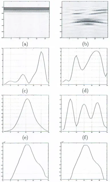
These four-channel of detection signals obtained from the full set of A-scans constitute the information that the detection will be carried on. In the appli­ cations of this algorithm, it has been observed that the reduction of the data from a full set of A-scans down to 4-chaimel of detection signals not only reduce the complexity of the detection but also made is more robust. In Figure 3.3. the raw B-scan together with its corresponding 4-channel of detection signals are shown. As seen from this figure, the detection signals capture the object scattered signal very efficiently.

In the remaining part of this section we will show how to use the detection signals to decide on those A-scans with little or no object scattered signals. As explained in the previous section, those A-scans with with little or no object- scattered signals are used in the update of the clutter signal s(x, y, t) in Equa­ tion 3.10. Reliability of the decision on whether an A-scan is of clutter signal only or not requires a statistical characterization of the clutter-only signals at an appropriate level of processing. For this purpose, the decision signals obtained at the output of the second-stage of processing can be used as fol­ lows. First form two fixed length sets for a given depth interval. One of these sets is composed of the selected correlation results Ck{xi,yi) corresponding to those locations (xi,yi) for which it’s decided that at these observation points the measured signal carries only the background information rc{xi,yut). This set will be denoted as Th corresponding to the k^''' depth interval. The second set is composed of the selected correlation results Ck{xi,yi) corresponding to

• ^ 25^ ■ '■ "■ .· i (a)' 20 40 so ftO 100 120 (b) (c ) (d) (f)

Figure 3.3: (a) Acquired raw B-scan measurement, (b) Object scattered sig­ nal estimate obtained by the first stage of processing. Depth dependent cor­ relations (a) Cl, (b) C2, (c)C3 and (d) C4 obtained by the second stage of processing.

those locations {xi,yi) for which it’s decided that at these observation points the measured signal carries the background information rc{xi,yi,t) plus some natural heterogeneity (plant roots, small stone particles, etc.). This set will be denoted as Aik corresponding to the depth interval.

Tk --= ■. i = 1,2, ....£} . k = 1,2,3,4 (3.25)

Afk -~ ■ * 1)2,. k = 1, 2,3,4. (3.26) The size of these sets, E is kept constant, during updating these sets, the oldest element is discarded. For initialization, both sets are assigned the first

E computed correlation results:

= { c k { x u y i ) : i ^ l ,2,...,E} , A: = 1,2,3,4 (3.27)

Mk = [Ck{xi,yi) -.1 = 1,2,...,E) , A: = 1,2,3,4. (3.28) When processing the data at the observation point {xi, yi), the update of both sets are done based on a hypothesis testing. For updating J^k and Mk, we define three hypotheses:

Ho : The A-scan is due to background scatter only.

Hi : The A-scan is due to scatter from the background with small scale inho­

mogeneities.

H2 : The A-scan is due to background and object scatter.

By assuming that the distribution of the correlation level under Hq has a nor­ mal distribution, we proceed the decision as follows: Let 71 and 72 be two parameters, if

||Cfc-iV ,|| X7i (3.29)

then the hypothesis Hq is true. If for all A:, (1 < A: < 4) at the point {xi,yi) then Tk is updated:

■ (3-30)

m

rrii^ = Ckix.y). (3.31)

Following this, the background signal s{t) is also updated as in equation 3.10. The updated signal s(x, y, t ) is fed back to the first stage of processing. Simi­ larly, if

IlCfc-iVfcll <a.v, X 72 (3.32) then the hypothesis Hy is true. If for all (1 < A: < 4) at the point {xi, yi) then Aik is updated:

rti, <r- n,_i

Tii^ = Cki x, y) .

(3.33) (3.34)

The parameters should be chosen carefully based on a statistical characteriza­ tion of actual set of measurements. Note that 71 and 72 should satisfy 72 > 7 i-The second set, A/k is used to determine the distribution of the correlation outputs when there’s no buried object. By this way, the expected level of correlations at the observation points (x,, y,) can be calculated and the

corre-I

lation results can be normalized with these numbers. The normalization allows us to produce decisions automatically. The normalization coefficients will be denoted as ^k und are computed as:

p

\nik\ TT'ii, ^ •iik· (3.35)

t=l

The normalized correlations are computed as:

Ck{i)

NCkii) = k = 1,2,3,4. (3.36)

On Figure 3.4 the normalized four level correlations obtained using the raw data displayed on Figure 2.3 is shown.

Figure 3.4: Normalized depth dependent correlations (a) A^Ci, (b) N C2·,

(c) NCz and (d) NC^ obtained by the second stage of processing.

At those measurement locations where there’s no object, the correlation result is expected to be on the order of 1. For a user unattended detection, the

K level informations need to be concatenated to form the input of an automatic

detection process. As part of the automatic detection process, the K level correlations are filtered with a median filter of length 2W + 1, and then filtered

results are thresholded with a pre-chosen threshold r. After thresholding, the results are averaged with the weighting coefficients which are chosen to be the normalization coefficients Formally, the steps of the automatic detection are: NCkit) = Med{NCk{i-W).,...,NCk{i:),...,NCk{i + W) } (3.37) P ^ k i i ) = 0, i f ] V C f c ( i ) < r . A; = 1, 2,3,4 Dr{x,y) = (3.3S) (3.39) A:=l

where Dr{x,y) is the compound processed decision signal which should be adaptively thresholded to decide on the existence and location of the objects. Choosing small values for r will result in noisier Dr{x-,y) signal, on the other hand larger values for r will decrease the contribution of object scattered in­ formation in Dr{x,y) signal. Therefore, multiple thresholds can be used and during the final stage of decision, the information in all of the decision signals can be fused for superior decision performance. In Figure 3.5 an illustrative example showing results of this processing is given.

i

(a) _(b)

(f)

Figure 3.5: Example: (a) Acquired raw B-scan measurement, (b) Object scattered signal estimate obtained by the first stage of processing. Normalized depth dependent correlations (a) NC\, (b) N C2, (c) N C3 and (d) NC^ obtained

by the second stage of processing, (g) Decision signal D2{x,y), dotted line is

the threshold, (h) Decision signal D4{x,y), dotted line is the threshold.

3.3 The third stage of processing of a GPR

measurement

In this section, we provide an automatic detection strategy which is aimed to detect the presence of buried objects on the decision signals Dr{x,y) generated by the second stage of processing. For simplicity we investigate the case of a single decision signal Dr{x,y)· The proposed detection strategy is chosen as an adaptive thresholding on the decision signal followed by a peak detector. The threshold is chosen adaptively by using the statistical characterization of the previously recorded measurements with no objects. Let {Dn{x.,y)} be set of measured images {1 < i < N) each of which corresponds to measurements with

no objects at the points {(xi, j/i), (2:2, 2/2)1 •••1 (xk^yk)}· Also let the average of these measurements be L·:

(Xk,yk)

A* = ^ ^ n ( x , y ) ·

(i,2/)=(ii,!/i) The decision threshold 7 is chosen as:

(3.40)

i — L p(j (3.41)

where, L is the sample mean, and <j/, is the standard deviation of Lf. 1 N

^

\

3.4 Considerations In The Real-Time Appli­

cation Of The Proposed Algorithm

In this section, the computational complexity of the algorithm will be investi­ gated to obtain the required processing power in a real-time application. After initializations are made, we will provide the number of multiplications needed to process one A-scan measurement before the nisxt measurement is acquired. F'or a particular A-scan measurement, the number of multiplications to produce a detection output for that measurement is found as follows: In the first stage of the proposed algorithm, time alignment is performed by a convolution oper­ ation between two signals of length tw as given in Equation 3.12. The number of multiplications in this operation is approximately ^^log-zitw)· Computa­ tion of a using Equation 3.15 needs (2iy -h 1) multiplications, where i/ is the length of the A-scan measurement vector and in practice i/ ~ At w Adaptive removal of clutter requires another tj multiplication (see Equation 3.13).

In the second stage of the algorithm, Ck{x,yys are com.puted using Equa­ tion 3.20. This operation requires 4 x 2 x M x ^ x 2 x W multiplications, where W is the output domain of the integral result in which the maximum will be assigned to Ck{x,y). In statistical analysis, computations of standard devia­ tions of the sets Tk ^ind J\fk require 4 x£^ multiplications, where E is the size of the sets Tk and

Mk-In the third and last stage of the algorithm, normalizations and producing the detection output requires a total of only 12 multiplications.

In total, the number of multiplications is given by:

No. of multiplications 4 X M X W X iy -|- 3 X iy "H 4 X Zi' -f 12. (3.45)

Typical values for the parameters are: tw = 64, tf = 256, M = 3, W = 5,

E = 8. So, in total around 2 x 10'^ multiplications is needed for processing one

A-scan. With today’s technology, allowing 100 Mips/sec/processor, required computation can be performed in about 0.2 msecs. This is far shorter than 5 msecs which is a typical time interval in between the acquisition of two consecutive A-scan measurements. Therefore the proposed algorithm is feasible to be implemented in real-time operations.

Chapter 4

RESULTS

In order to asses the performance of the proposed algorithm in various practical scenarios, tests are performed on two groups of measurement data. The first group of data is produced via simulating the GPR measurements using the finite difference time domain technique for solving Maxwell equations. [17] The second group of data is acquired at the testing bed in Tiibitak Marmara Research Center [18].

4.1 Simulation Based Results

The GPR measurement is simulated via FDTD analysis methods [17] developed by the computational electro magnetics (GEM) research group of Bilkent Uni­ versity. To obtain results closer to the reality, various scenarios including the propagating media to be defined as lossy and having random inhomogeneities

are prepared. In the simulated scenarios, the GPR unit realizes a linear sur­ vey, in the X direction, therefore there’s no y component dependence. In all of the simulations, there’s one object located at the center of the observation measured earth. Upon applying the proposed processing approach, it is ob­ served that background clutter removal is successful in all cases. Detection is succeeded in all cases where the signal due to the inhomogeneities doesn’t dominate the object signal.

On each set of scenarios 8 figures are plotted. The first image is the raw B-scan. The second image is the processed B-scan. The following four figures show the depth dependent normalized correlation results, NC\^ N C2, NCz,

and NCi[ respectively. The last figure shows the thresholded detection outputs £>2(3;) and D4{x).

The threshold for detection is computed using the detection outputs D{x) at which the received signal includes little or no object scattered signal. For the cases shown in Figures 4.1 - 4.7 the detection threshold is computed as 72 = 3.2510^ and 74 = 2.8910^ for r = 2 and r = 4, respectively. For the cases shown in Figures 4.12 - 4.15 the threshold is set to 72 = 2.7010'* and

74 = 1.7910“* for r = 2 and r = 4, respectively.

In Figure 4.1, results of performing the proposed algorithm on the sim­ ulated GPR measurement corresponding to a cylindrical non-metallic object with diameter = 5 cm and height = 4cm, buried at 8 cm below the surface is given. The ground is modeled as homogeneous and lossless, i.e. ideal. The object is detected at the first depth level.

In Figure 4.2, again results of performing the proposed algorithm on the simulated GPR measurement corresponding to a cylindrical non-rnetallic object with diameter = 5 cm and height = 4cm, buried at 8 cm below the surface is given. This time the ground is modeled as lossless but heterogeneous. The object is again detected at the first depth level.

In Figure 4.3, results of performing the proposed algorithm on the simu­ lated GPR measurement corresponding to a non-rnetallic 5 cmx5 cmx4 cm prism buried at 2 cm below the surface is given. The ground is modeled as heterogeneous and lossy with a = 0.1 S/rn The object is successfully detected at the first depth level.

In Figure 4.4, results of performing the proposed algorithm on the simu­ lated GPR measurement corresponding to a non-metallic 5 cmx5 cmx4 cm prism buried at 15 cm below the surface is given. The ground is modeled as heterogeneous and lossy with a = 0.1 S/rn The object is detected with less success, also a false detection is made.

In Figure 4.5, results of performing the proposed algorithm on the simu­ lated GPR measurement corresponding to a non-metallic 5 crnx5 cmx4 cm prism buried at 8 cm below the surface is given. The ground is modeled as heterogeneous and lossy with a = 0.1 S/rn The object is detected successfully at the third depth level.

In Figure 4.6, results of performing the proposed algorithm on the simu­ lated GPR measurement corresponding to a non-metallic 5 cmx5 cmx4 cm prism buried at 8 cm below the surface is given. The ground is modeled as

heterogeneous and lossy with a = 0.15 S/in The object is detected at tlie third depth level.

In Figure 4.7, results of perforniing the i)roposcd algorithm on the simu­ lated GPR measurement corresponding to a non-rnetallic 5 cmx5 cmx4 cm prism buried at 8 cm below the surface is given. The ground is modeled as heterogeneous and lossy with a = 0.20 S/rn The object could not be detected.

In Figures 4.12 - 4.15, results of performing the proposed algorithm on the simulated GPR measurement corresponding to a cylindrical non-rnetallic object with diameter = 5 cm and height = 4crn, buried at 8 cm below the surface is given for 4 different ground models. In Figures 4.8 - 4.11 the ground models are shown. In all cases, the object is detected successfully. The most successful detection is performed for the ground model 4.8, for which the amount of heterogeneity is the least.

(a) (b)

( f)

(g)

Figure 4.1; GPR image obtained by simulation. The ground is modeled as homogeneous, and lossless. The object is a cylindrical plastic object with diameter = 5cm with relative dielectric constant e = 3. The ground dielectric constant is chosen to be e = 8. The top of the object is 8 cm below the surface, (a) Acquired raw B-scan measurement, (b) Object scattered signal estimate obtained by the first stage of processing. Normalized depth dependent correlations (a) NCi, (b) N C2, (c) N0·^ and (d) NC/i obtained by the second

stage of processing, (g) Decision signal D2{x,y), dotted line is the threshold,

(h) Decision signal D^{x,y), dotted line is the threshold.

(f)

Figure 4.2: GPR image obtained by simulation. The ground is modeled as heterogeneous, but lossless. The object is a cylindrical plastic object with diameter = 5cm with relative dielectric constant e = 3. The ground dielectric constant is chosen to be e = 8. The top of the object is 8 cm below the surface, (a) Acquired raw B-scan measurement, (b) Object scattered signal estimate obtained by the first stage of processing. Normalized depth dependent correlations (a) A^Oi, (b) N C2·, (c) NCz and (d) NC^ obtained by the second

stage of processing, (g) Decision signal T>2(.x,y), dotted line is the threshold, (h) Decision signal D^{x,y), dotted line is the threshold.