Analyzing the forecast performance of S&P 500 Index Options implied volatility

ANALYZING THE FORECAST PERFORMANCE OF S&P 500 INDEX OPTIONS IMPLIED VOLATILITY

A Master’s Thesis by AYTAÇ ERDEMİR Department of Management

İhsan Doğramacı Bilkent University Ankara

ANALYZING THE FORECAST PERFORMANCE OF S&P 500 INDEX OPTIONS IMPLIED VOLATILITY

Graduate School of Economics and Social Sciences of

İhsan Doğramacı Bilkent University

by

AYTAÇ ERDEMİR

In Partial Fulfillment of the Requirements for the Degree of MASTER OF SCIENCE

in

THE DEPARTMENT OF MANAGEMENT

İHSAN DOĞRAMACI BİLKENT UNIVERSITY ANKARA

I certify that I have read this thesis and have found that it is fully adequate, in scope and in quality, as a thesis for the degree of Master of Science in Business Administration.

---

Assoc. Prof. Dr. Aslihan Altay Salih Supervisor

I certify that I have read this thesis and have found that it is fully adequate, in scope and in quality, as a thesis for the degree of Master of Science in Business Administration.

--- Prof. Dr. Ümit Özlale

Examining Committee Member

I certify that I have read this thesis and have found that it is fully adequate, in scope and in quality, as a thesis for the degree of Master of Science in Business Administration

---

Assoc. Prof. Dr. Levent Akdeniz Examining Committee Member

Approval of the Graduate School of Economics and Social Sciences

--- Prof. Dr. Erdal Erel Director

ABSTRACT

ANALYZING THE FORECAST PERFORMANCE OF S&P 500 INDEX OPTIONS IMPLIED VOLATILITY

Erdemir, Aytaç

M.S., Department of Management

Supervisor: Assoc. Prof. Dr. Aslıhan Salih Altay

September 2012

This study examines the comparative performance of the call and put implied volatility (IV) of at-the-money European-style SPX Index Options on the S&P 500 Price Index as a precursor to the ex-post realized volatility. The results confirm that implied volatility contains valuable information regarding the ex-post realized volatility during the last decade for the S&P 500 market. The empirical findings also indicate that the put implied volatility has a higher forecast performance. Furthermore, from the wavelet estimations it has been concluded that the long-run variation of the implied volatility is consistent and unbiased in explaining the long-run variations of the ex-post realized volatility. Wavelet estimations further reveal that in the long-run put and call implied volatility contain comparable information regarding the realized volatility of the market. However, in the short-run put implied volatility dynamics have better predictive ability.

ÖZET

S&P 500 ENDEKS OPSIYONLARI İÇSEL OYNAKLIĞININ TAHMİN ETKİNLİĞİNİN İNCELENMESİ

Erdemir, Aytaç

Yüksek Lisans, İşletme Bölümü

Tez Yöneticisi: Assoc. Prof. Dr. Aslıhan Salih Altay

Eylül 2012

Bu çalışma S&P 500 Endeksi üzerindeki Avrupa-tipi SPX al ve sat opsiyonları içsel oynaklığının, gelecek piyasa volatilitesini karşılaştırmalı tahmin performansını incelemiştir. Sonuçlar, geçen on yıl boyunca opsiyon içsel oynaklıklarının S&P 500 gelecek piyasa volatilitesini açıklamada değerli bilgi içerdiğini doğrulamaktadır. Sonuçlar ayrıca, sat endeks opsiyonlarından elde edilen içsel oynaklığın daha yüksek bir tahmin performansına sahip olduğunu göstermektedir. Ayrıca, dalgacık hesaplamalarından opsiyon içsel oynaklığının uzun-vadeli değişiminin, gelecek piyasa volatilitesi değişimini açıklamada uzun vadede tutarlı ve eğilimsiz olduğunu ortaya koymaktadır. Dalgacık hesaplamaları uzun vadede al-sat opsiyonları oynaklıklarının piyasanın realize edilen oynaklığı için karşılaştırılabilir bilgi içerdiğini göstermektedir. Ancak, kısa vadede sat opsiyon oynaklığının tahmin becerisi daha iyi olmaktadır.

ACKNOWLEDGEMENTS

I would like to express my deepest gratitude to my supervisor Professor Aslıhan Altay Salih for her guidance, support and understanding.

I would like to convey my thanks to Professor Ümit Özlale for his invaluable suggestions and criticism.

I would also like to thank all jury members for reading and giving valuable comments for this thesis.

I am also thankful to Rabia Hırlakoğlu for her kindly assistance during the M.S. program.

TABLE OF CONTENTS

ABSTRACT ... iii

ÖZET ... iv

ACKNOWLEDGEMENTS ... v

TABLE OF CONTENTS ... vi

LIST OF TABLES ... viii

LIST OF FIGURES ... ix

CHAPTER 1: INTRODUCTION ... 1

CHAPTER 2: LITERATURE REVIEW ... 8

CHAPTER 3: DATA AND PRELIMINARY ANALYSIS ... 15

CHAPTER 4: STANDARD ECONOMETRIC MODELS ... 24

4.1. Least Squares Estimation ... 26

4.2. Forecast Performance ... 32

CHAPTER 5: WAVELET DECOMPOSITION ... 36

LIST OF TABLES

Table 1. Thomson Reuters DataStream Option Models ... 16

Table 2. Descriptive Statistics for Raw Data ... 17

Table 3. Descriptive Statistics for Log Data ... 19

Table 4. Information Content of the Implied Volatility: Least Squares Estimates ... 29

Table 5. Comparison of Forecast Performances ... 33

Table 6. Time Scales ... 43

Table 7. Energy Levels ... 48

Table 8. Descriptive Statistics for Realized Volatility Scales ... 48

Table 9. Descriptive Statistics for Put Implied Volatility Scales ... 49

Table 10. Multi-scale Regressions for Put Implied Information Content ... 51

LIST OF FIGURES

Figure 1. S&P 500 Price Index Realized and Call Implied Volatility ... 20

Figure 2. S&P 500 Call & Put Implied Volatility ... 21

Figure 3. ACF and PACF of S&P 500 Volatility ... 22

Figure 4. Partitioning of Time-Frequency Plane by Different Methods ... 39

Figure 5. Wavelet Decomposition ... 40

Figure 6. Symlet-8 Wavelet Family: Wavelet and Scaling Functions ... 43

Figure 7. Realized Volatility and Approximation Level ... 44

Figure 8. Implied Volatility (Put) and Approximation Level ... 45

Figure 9. Approximation Level ... 45

Figure 10. 3rd Detail Level ... 46

Figure 11. 2nd Detail Level ... 46

CHAPTER 1

INTRODUCTION

In finance, forecasting volatility is deemed as an important task, and the ever-growing financial markets stimulate an extensive research focus on this task. While finance professionals investigate the forecasting performance of different volatility models, scholars pay a special interest for understanding the structure and the efficiency of the implied volatility in estimating the future realized volatility of the related market.

In this regard, the thesis examines the performance of the call and put implied volatility (IV) of at-the-money (ATM) SPX options on the S&P 500 Index in estimating volatility from May 2001 until January 2012.

First, I utilize the classical least squares method for the very basic regression models, in which I seek to analyze the relation between realized volatility and implied volatility.

Then, I examine the simultaneous equation model proposed by Christensen and Prabhala (1998) and Christensen and Hansen (2002). Secondly, the wavelet decomposition method, proposed specifically for financial time series by Ramsey (2002), to account for the time series and frequency domain dynamics of volatility series.

The least squares model yields more consistent and significant results than the previously proposed simultaneous system. The explanatory power and forecasting ability of the implied volatility is overall very significant for the S&P 500 over the last ten years. The put implied volatility is superior when compared with the call implied volatility. Moreover, the call implied is superior than the historical volatility in explaining the ex-post realized volatility. The empirical results from the wavelet decomposition take this analysis to a step further and reveal a brighter picture about the option implied volatility. Results indicate that volatility implied from the S&P 500 Index options contain valuable information in explaining the future realized volatility especially for the long-term.

Volatility is the core measure of uncertainty in markets. It is an input for pricing the financial derivatives, for investment decisions and for risk management practices. In reality, the term ‘volatility’ represents two distinct classifications as follows:

a. Historical or realized volatility: It is a backward-looking measure and usually measured as the standard deviation of price changes at different time intervals. b. Implied volatility: It is considered a forward-looking measure, is derived from

To be more precise, implied volatility refers to the average volatility forecast over the option maturity, or as the overall expectation of the future volatility of the whole market, including all agents. From the rational expectations perspective, markets use all available information available to form their estimation of the future volatility. Correspondingly, the market option price reveals the markets’ assessment of the underlying asset’s volatility over the option maturity. This means that implied volatility must be an unbiased and efficient predictor of future realized volatility during the life of the option (Christensen and Hansen, 2002).

Granger and Poon (2003) explain that using the implied volatility of at-the-money (ATM) call (and put) options have two grounds: first, the liquidity of the ATM options and second, trying to minimize the effect of volatility smile will only be possible by choosing ATM implied volatility.

This study demonstrates the forecast ability and significance of the ATM implied volatility information content for the future volatility realizations for the S&P 500 Index. The research motivation of this study is to investigate the relationship between the implied volatility of the index options of the benchmark stock index and the ex-post realized volatility (of the underlying benchmark), and to determine the contemporary dynamics of this relationship during the last decade. Moreover, we evaluate the forecast performance of implied volatility. While the previous studies have contradictory findings, which I will explain in the next chapter, this work differs from prior studies from a number of aspects.

First, the empirical findings demonstrate the forecast ability and the significance of information content in the implied volatility. Secondly, the put and

call implied volatility comparison have revealed some interesting facts. The trading volume of the options has been globally increasing in general, but the expansion of trading volume of S&P Index options is remarkable. Indeed, the Chicago Board Options Exchange (CBOE) reports that S&P 500 Index Option volume has exponentially increased over the last ten years supporting liquidity. The put options are liquid derivatives that can limit the downside risk for the market. If the market volume has increased that much, it means that the hedging activities have increased. Hence, if the implied volatility represents the expectations of the market, then the put implied volatility must be a comparatively better forecast as it is used as a principal hedging instrument against exposure to the S&P 500 Index. In that regard, we indeed compare and confirm the higher performance of the put implied.

Another improvement of this study stems from the standardized market facts. CBOE Market Statistics for 2001 indicates an annual dollar volume of about $7.8 billion for OEX (S&P 100) American style options and $5.6 billion for SPX (S&P 500) European style options. Yet for 2011, CBOE reports an annual dollar volume of about $485.7 billion for SPX and $3.3 billion for OEX options, respectively. The fact that the previous studies examining the forecast performance of implied volatility have mostly used implied volatility from American-style index options, e.g. OEX, can be referred as a crucial shortcoming. This study contributes to the literature by investigating the ability of call and put volatility implied by liquid SPX European type Index options. This can be referred as another significant advantage when compared with the prior studies.

Another contribution of this study is related with the time series features of the volatility. The apparent market dynamics imply that, utilizing a multi-scale

analysis of the volatility of the market might allow us to discover different characteristics that are prevalent for different periods. For this reason, the wavelet decomposition method is applied and the implied versus realized volatility dynamics has been considered for the long, medium and short term.

In the academic literature the wavelet methodology have been implemented in a number of studies to analyze the features of financial and economic time series, including volatility, and their corresponding relationships. Gencay et al (2011), for instance, investigate the asymmetry of information flow between volatilities. Nevertheless, this study uses the wavelet technique to scrutinize the implied and realized volatility relationship. Hence, this brings an innovative perspective to the relevant literature.

In addition, the distinct relationship characteristics between the implied and realized volatility for different periods support the heterogeneous markets hypothesis of Müller et al. (1997). That is, analyzing different components of the volatility that are prevalent for different periods.

Heterogeneous markets hypothesis acknowledge that any financial market is comprised of distinct agents with different investment horizons and different risk exposures resulting from that horizon. Müller et al. (1997) emphasize that we need to adopt an alternative approach in volatility characterization, an approach that does not assume a uniform volatility (or risk) exposure for all agents. According to the authors, different agents must estimate and consider different volatility measures depending on their horizons. This is another aspect of including the robust wavelet multi-scale decomposition technique in this research.

The empirical results from the wavelet decomposition technique are in alignment with the findings of the recent studies of Busch et al. (2011) and Dufour et al. (2012). Busch et al. (2011) propose a vector heterogeneous autoregressive model (VecHAR) to decompose the volatility components. They find that the implied volatility contain incremental information about future volatility. They conclude that implied volatility should be used in forecasting future realized volatility. They also add that the implied volatility can even predict the jump component, which corresponds to high frequency component in our case, to some extent. Further, Dufour et al. (2012) considers that the informational value of implied volatility also capture the realized implied relationships, i.e. as the leverage effect of the volatility feedback. They also claim implied volatility forecast contains the variance risk premium of the market. When we look at the long-term coefficient of the call and put implied volatility, our results may be related with this finding.

In sum, this study empirically represents the crucial feature of put and call implied volatility for all S&P 500 market. We clarify the forecast capability and dynamics of implied volatility by allowing comparative analysis. Few studies claim that implied is an unbiased and efficient forecast of the ex-post realized index volatility of the S&P 100 Index after the 1987 stock market crash (Christensen and Prabhala 1998, later Christensen and Hansen 2002). Some define it as a powerful, upward-biased predictor of the future realized volatility (Fleming, 1998). Yet, the prior implications are deducted from studying the market during the 90s, especially after the market crash of 1987.

While it is an evident necessity to evaluate the efficiency of implied volatility for the last decade, the time varying characteristics of volatility have been

continuously confirmed in a number of seminal papers, such as Mandelbrot, 1963; Fama, 1965; Engle, 1982; Bollerslev, 1986 and so on. Mandelbrot (1963) and Fama (1965) for instance, were the first to bring the heteroscedasticity and significant excess kurtosis issue in the first differences of logarithms of stock prices. This study is innovative to fuse a competent analysis technique to enlighten the comparative short-term and long-term dynamics of volatility time series.

Frankly, the volatility forecasting studies are all bound to constraints and limitations that originate from the heterogeneous and time varying characteristics of volatility. Moreover, it is crucial to comprehend the features of the data together with the explicit and implicit deductions of the econometric tools and models in investigating the implied volatility. The growing academic literature on this matter, accordingly, focuses more on discovering the behavior of the time series, questions the unrealistic constraints.

The plan of the thesis is as follows: The second chapter explains the relevant academic background of this study. Then, third chapter reveals data and preliminary results. In the Chapter 4, the econometric models have been investigated via least squares regressions. Then the forecast performances have been evaluated. Chapter 5 explains the wavelet decomposition method and the multi-scale properties of implied and realized volatility time series, and discusses their relationship under such a framework. The last chapter summarizes the empirical results and explains the crucial implications for the market.

CHAPTER 2

LITERATURE REVIEW

In the last decades, a myriad of studies have investigated the information content and the forecast ability of the implied volatility and the relationship of implied and future realized volatility. In that respect, there is no consensus in the finance literature and presented empirical findings and assertions have two contradictory stances.

One line of research considers the implied volatility as an efficient forecast of future expectations. In that regard for instance, some earlier studies give credit to the explanatory ability of implied volatility (such as Latane and Rendleman, 1976; and Chiras and Manaster, 1978). In contrast, the other line of research, studies like Canina and Figlewski (1993), assert the exact opposite of the assertion and denounce the forecast ability of implied volatility. Canina and Figlewski, particularly, analyze the regression of monthly volatility forecasts by one-month OEX implied volatilities on S&P 100 index options and on past S&P 100 index volatility. They conclude that implied volatility is of no use as a predictor of

ex-post volatility and it is dominated by historical volatility measure.

Then, Jorion (1995) focuses on foreign exchange (FX) market. He claims that the measurements of implied volatility of FX options are less prone to bias. He concludes that implied volatility is a biased yet superior forecast. Later, Vasilellis and Meade (1996) assert that the implied stock volatility from option prices is an efficient forecast for future volatility. They also advocate combining implied and GARCH volatility forecasts. However, the value of ARCH/GARCH type models has been put into question by other papers. Pagan and Schwert (1990) and Loudon et al. (2000), for example, have demonstrated that the use of ARCH/GARCH type models tends to produce bias in volatility predictions. Similarly, Engle and González-Rivera (1991) and Bollerslev and Wooldridge (1992) have shown estimation problems related to the hypotheses made about the distributions of error terms of such models and indicate that these problems would explain the biases observed in predictions of volatility.

Furthermore, it has been unveiled by other seminal studies that implied volatility often outperforms time-series approaches (e.g. ARCH/GARCH type models) by presenting empirical results from the S&P Index; particularly Fleming (1998), Blair et al. (2001), Hol and Koopman (2002).

In the prominent Journal of Financial Economics paper “The relation between implied and realized volatility” by B.J Christensen and N.R Prabhala (1998), authors use OEX (S&P 100) American-style index options implied volatility to forecast the future realized volatility. They say that implied volatility is efficient in forecasting the future market volatility and it is unbiased. Their study differs in

the sense that they reject the bias and claim that the auto-correlated residual structure is caused by the measurement errors. Christensen and Prabhala also claim that, if the potential errors-in-variables problem can be eliminated by data adjustment, the degree of bias in implied volatility forecasts will be much less, than previous research studies in literature. Following their work, more recent studies, such as Hansen (2001) for Danish KFX index options, Christensen and Hansen (2002) for S&P 100 index options, Shu and Zhang (2003) for S&P 500 index options, and Szakmary et al (2003) for futures options, view implied volatility as a better forecast of future realized volatility than historical volatility.

At the same time with the study of Christensen and Prabhala, another remarkable paper by Fleming (1998) finds similar results with a small difference. Fleming also uses OEX implied volatility and uses the Generalized Method of Moments technique to eliminate the serial correlation and heteroskedasticity problem. Similar to Jorion (1995) they found that the implied volatility includes all the information from historical volatility; hence, it is an upward biased forecast of future volatility of the S&P 100 market. These results are claimed to be consistent for up to several-month length forecast horizons.

While the financial literature expands with numerous studies on volatility modeling and studying the forecasting performance of those models, Müller et al. (1997) have incorporated the heterogeneous market hypothesis with the volatility modeling in their revolutionary Journal of Empirical Finance paper. They measure volatilities of the foreign exchange market on different time resolutions and compare them in a lagged correlation study. They discover that the long-term volatility predicts short-term volatility significantly better. They conclude that the

resolution of statistical volatility computation is an essential parameter which reflects the perception and the actions of different market components from short-term to long-term traders. They emphasize the asymmetric information flow between non-homogeneous traders. By asymmetry, they refer to the phenomena that short-term traders react to long-term volatility by increasing their trading activity, thus have an effect on short-term, whereas long-term traders mostly ignore the short-term volatility.

The long memory of volatility, described in Dacorogna et al. (1993) and Ding et al. (1993), is explained in terms of different market participants with different time horizons. Andersen and Bollerslev (1997) also underline the long memory property of the volatility. Mandelbrot (1963) was among the first to describe the clustering as subsequent large changes, or subsequent small changes. Dacorogna et al. (2001) much later explains in detail the time-dependent characteristics and idiosyncrasies of the volatility. They further underline that the autocorrelation of the absolute value of returns indicate long memory effects. Moreover, Dacorogna et al. (2001) measure the lagged correlations of mean volatility time series at different time resolutions, and infer that an asymmetric information flow structure exists, and long-term volatility better predicts the future and short-term volatility too. Briefly, it can be deducted that their study is in alignment with the framework proposed by Müller et al. (1997).

In accordance with these aforementioned studies, Selçuk and Gencay (2006) point out the nonlinear scaling feature of moments across time scales, describing it as the essential dynamic feature of financial time series. They also note that each moment scales nonlinearly at a different rate across each time scale. This, they

interpret, prohibits popular continuous time representations, such as Brownian motion, as possible candidates in explaining return dynamics.

In sum, while the overall a review of the literature appears to be away from a consensus, it is a tentative conclusion that implied volatility does provide a better forecast or guide for future volatility than forecasts based solely on historical information.

Nevertheless, the empirical evidence on this strong assertion is limited. From a literary perspective, this thesis contributes to the existing financial literature by bringing a novel perspective to the posit stating that implied volatility may be used as a proxy for market-based volatility forecast. Initially, it expands the previous studies on forecasting ability of volatility on the S&P 500 Index to cover the last decade, a period of unforeseen financial crises, and compares the hypotheses and results of standard econometric models. The hypotheses all describe a linear dependence structure between the implied and ex-post realized volatility, and claim that implied volatility contains information about future realized volatility. The results of the standard econometric models have been compared with the previous findings of Christensen and Prabhala (1998) and Christensen and Hansen (2002).

Secondly, it scrutinizes the wavelet decomposition methodology to estimate different components of volatility on different time horizons. Wavelet methodology is suitable because it does not distort the examined time series data. Dealing with the non-stationary, or near unit root data is a delicate matter. Academic background on financial time series explicitly state that all financial returns have non-stationary

volatilities (Aït-Sahalia and Park, 2012).

Moreover, by analyzing the forecasting ability of the implied volatility with wavelet decomposition, we target try to disclose the importance of heterogeneous market agents, and whether exposure to different volatility components matter for those agents. The empirical findings elucidate whether long-term volatility or short-term realized and implied volatilities have different dynamic relationships, if so should agents change their investment decisions with respect to their exposure term. Concisely, for these reasons, it is believed that this thesis provides a better understanding of the dynamic properties of contemporary, post-millennia implied volatility, thereby helps expanding the literature on volatility forecasting.

Recently, Busch et al. (2011) find that the implied volatility contains valuable information about the future volatility in stock markets, and it is an unbiased forecast. They separate the volatility series into smooth and jump components, jump components representing the high-frequency changes in the short-term. They conclude that implied volatility predicts the overall future realized values of volatility for the stock market, and efficiently predicts the smooth part of the future volatility. In addition, they underline that the implied volatility can even explain the jump components of the future realized volatility up to some extent. The wavelet decomposition technique will specifically allow us to evaluate this assertion for the S&P 500 market during the last decade.

Similarly, Dufour et al. (2012) find that volatility feedback effect on the S&P 500 market works through implied volatility, with its nonlinear and forward-looking relation with option prices. They further conclude that observing the volatility

feedback effect at different horizons, i.e. short-run and long-run, can be attributed to the power of implied volatility to predict future volatility. In sum, their detailed analyses on the implied and realized volatility support the forecast ability of the implied volatility to predict future volatility of the market.

CHAPTER 3

DATA AND PRELIMINARY ANALYSIS

The data set analyzed in this study is based on the S&P 500 Price Index monthly return. The time series have been observed during the period of May 2001 to January 2012. Pt denoting the price of S&P 500 at month t, the average monthly return is calculated by;

1 t t t P R ln P− = _ _  _

The time series of realized volatility is calculated by the estimator of standard deviations of monthly returns. Christensen and Prabhala (2002) describe implied volatility as the ex-ante volatility forecast, and they calculate the ex-post realized return volatility over the monthly option period. Accordingly, the series for realized volatility is estimated as the daily index return standard deviation

over the remaining life of option, as follows: 2 , , 1 1 t _{( )} h t t k t k t R R τ σ τ = =

∑

Where τ is the number of days until the month’s end, t

, 1

1 t _{( )}

t _k t k t

R =_τ

∑

implied volatility is expressed in annual terms, the realized volatility measure is also quotes as annual terms.

While the realized volatility of the underlying, i.e. S&P 500 Index time series is calculated as follows, the implied volatility data used in the study is obtained from the Thomson Reuters DataStream implied call ( c

t

σ ) and implied put volatility ( p

t

σ ) on the S&P 500 Index. The Thomson Reuters DataStream report (2008) that in February 2000, they enhanced and standardized the options models as such:

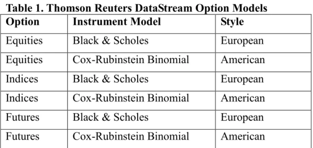
Table 1. Thomson Reuters DataStream Option Models

Option Instrument Model Style

Equities Black & Scholes European Equities Cox-Rubinstein Binomial American Indices Black & Scholes European Indices Cox-Rubinstein Binomial American Futures Black & Scholes European Futures Cox-Rubinstein Binomial American

Since the American-style options can be exercised early but European-style options only on expiry, the Cox-Rubinstein Binomial model depicts a binomial tree backwards looking at each step whether exercise is optimal. Thomson Reuters DataStream also points out that all Index options are European-style (except one LSX – FTSE100), whereas all equity, bond, and for-ex options are American style. In addition, they explain that at-the-money implied volatilities are estimated by interpolating between the two nearest strikes and at the money strike using values from the nearest expiry month options. The series switches to the next available month on the first day of the expiry month. Therefore, the horizon of the implied volatility is monthly. Given these properties, Table 2 gives the descriptive statistics for the raw data in monthly terms.

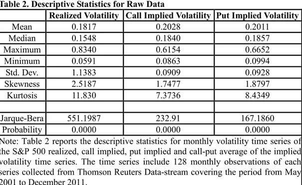
Table 2. Descriptive Statistics for Raw Data

Realized Volatility Call Implied Volatility Put Implied Volatility

Mean 0.1817 0.2028 0.2011 Median 0.1548 0.1840 0.1857 Maximum 0.8340 0.6154 0.6652 Minimum 0.0591 0.0863 0.0994 Std. Dev. 1.1383 0.0909 0.0928 Skewness 2.5187 1.7477 1.8797 Kurtosis 11.830 7.3736 8.4349 Jarque-Bera 551.1987 232.91 167.1860 Probability 0.0000 0.0000 0.0000

Note: Table 2 reports the descriptive statistics for monthly volatility time series of the S&P 500 realized, call implied, put implied and call-put average of the implied volatility time series. The time series include 128 monthly observations of each series collected from Thomson Reuters Data-stream covering the period from May 2001 to December 2011.

We can see that the average realized volatility is lower than the average call and put implied volatility. This reality can be attributed to the presence of a volatility premium for the S&P 500. Another important deduction is about the distributions of the series. The skewness and kurtosis roughly describe the shape of

the distribution of the data. To be more precise, values of skewness and kurtosis reveal the asymmetry and the tail thickness of the market return distributions, respectively.

The kurtosis values of 11.83 for realized volatility, and 7.37 for call implied and 8.43 for put implied indicate that the distribution of the series are not normal. Kurtosis values indicate presence of leptokurtosis, or fat tails, which means that the distribution has more probability mass in the tails than the normal distribution. In addition, one can observe that the realized volatility series is more skewed and more leptokurtic than the implied volatility series.

The Jarque-Bera normality test statistic aggregate both skewness and kurtosis information of the data and produces a test for normality. When we look at the Jarque-Bera statistics, we reject the null hypothesis of normal distribution within the 1% significance level. Therefore, using raw data for our models would be a major drawback, due to the failure of the normality assumption proven by the Jarque-Bera test statistics.

Furthermore, we have investigated the long memory property, also described as persistence or long-range dependence. Essentially, the long memory property implies that past events have a decaying effect on the future of the series. The long memory property of a time series is determined by calculating the Hurst exponent. In finance literature, Mandelbrot (1972) especially showed that the the Hurst estimator detects dependence, even in the presence of significant excess skewness or kurtosis and it can catch the non-periodic cycles. He said that the Hurst exponent H=0.5 would indicate independent processes, though it can be non-Gaussian

process.

Empirical results give a Hurst estimate of 0.8607 for S&P 500 realized return and 0.9210 for the implied volatility. Results can be interpreted as a demonstration of the long-memory or persistence property of the volatility for the period of March 2001 to January 2012. Alternatively, it can be interpreted as periods of high-volatility will tend to be followed by high-volatility, and low-volatility periods will tend to be followed by low-low-volatility periods. This finding can be a confirmation of clustering property of the volatility series.

In order to overcome the significant level of skewness and excess kurtosis, we have calculated the log-transformed series. Like the prior studies of Christensen and Prabhala (1998) and Christensen and Hansen (2002), we decided to use the log-transformed data. The descriptive statistics are summarized in Table 3.

Table 3. Descriptive Statistics for Log Data

Log Realized Volatility Log Implied Volatility (Call) Log Implied Volatility (Put) Log Implied Volatility (Average) Mean -1.8551 -1.6876 -1.6800 -1.6838 Median -1.8652 -1.6832 -1.6928 -1.6850 Maximum -0.1814 -0.4855 -0.4075 -0.4465 Minimum -2.8275 -2.4492 -2.3081 -2.3500 Std. Dev. 0.5250 0.4004 0.4009 0.3994 Skewness 0.5474 0.4473 0.4884 0.4728 Kurtosis 3.1954 2.9085 2.9326 2.9128 Jarque-Bera 6.5966 4.3129 5.1120 4.8092 Probability 0.03695 0.11573 0.07761 0.0903

Note: Table 3 reports the descriptive statistics for the natural logarithm of the

monthly S&P 500 realized, call implied, put implied and call-put average of the implied volatility time series. It is based on 128 monthly observations on each volatility series collected from Thomson Reuters Data-stream covering the period from May 2001 to December 2011.

From Table 3, we can conclude that we cannot reject the null hypothesis of normal distribution for all realized and implied volatility time series within the 1% significance level. It is an important conclusion since in the next Chapters the models and statistical interpretations of the models that have been tested are more powerful under the normality assumption.

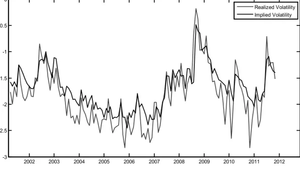
The Figures 1 and 2 show the monthly S&P 500 realized, put and call implied volatility series graphically. It should be noted that all the estimations are based on the log-transformed time series from this point on. Therefore, the following figures are describing the log-transformed data.

Figure 1. S&P 500 Price Index Realized and Call Implied Volatility

2002 2003 2004 2005 2006 2007 2008 2009 2010 2011 2012 -3 -2.5 -2 -1.5 -1 -0.5 0 Realized Volatility Implied Volatility

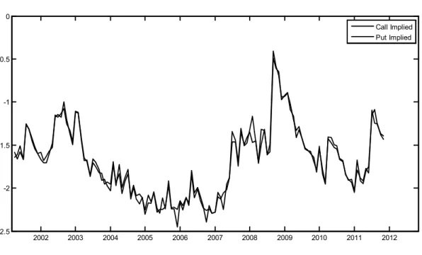
Figure 2. S&P 500 Call & Put Implied Volatility 2002 2003 2004 2005 2006 2007 2008 2009 2010 2011 2012 -2.5 -2 -1.5 -1 -0.5 0 Call Implied Put Implied

One can notice from Figure 2 that the log-transformed call and put implied volatility time series are very close. Since the implied volatility is valid for monthly duration, using monthly-calculated values would eliminate any duration related problem in general. Still, we should keep in mind that all quoted volatility series are merely estimations and time series values calculated as defined previously.

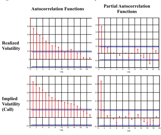
In addition to Jarque-Bera, we have checked for the serial correlation. Autocorrelation, also known as serial correlation, is the correlation of the variable with its past values. It can be a significant problem for the regression analysis. To check for autocorrelation the autocorrelation function (ACF) and the partial autocorrelation function (PACF) are estimated. The Figure 3 shows the ACF and PACF of the realized and implied volatility. The figure shown below indicates that the series appear as stationary autoregressive time series.

Figure 3. ACF and PACF of S&P 500 Volatility

Autocorrelation Functions Partial Autocorrelation _Functions

Realized Volatility 0 2 4 6 8 10 12 14 16 18 -0.2 0 0.2 0.4 0.6 0.8 Lag Sample Autocorrelation Function

0 2 4 6 8 10 12 14 16 18 20 -0.4 -0.2 0 0.2 0.4 0.6 0.8 1 Lag p p Implied Volatility (Call) 0 2 4 6 8 10 12 14 16 18 -0.2 0 0.2 0.4 0.6 0.8 Lag 0 2 4 6 8 10 12 14 16 18 20 -0.2 0 0.2 0.4 0.6 0.8 Lag p

From the descriptive data analysis, it can be concluded that the log-transformed series would be appropriate to investigate the explanatory relationships. However, while the data characteristics conform to our econometric examination, that the true market volatility is not observable (Fleming, 1998) It is a challenging fact about the time series analysis of the volatility. It has been acknowledged that various measures for volatility, such as standard deviations, variance, or absolute values of returns are proxies for the true market volatility and our calculations are such proxies that are bound to constraints and measurement errors emerging from the estimated data (Ding, Granger and Engle, 1993; Fleming, 1998; Christensen and Prabhala, 1998; Granger and Pool, 2003).

It means that independent from the estimation technique we have chosen to represent the realized volatility value, what we really use are different representatives, or proxies estimated from the earlier sets of observations. This can be referred as the unobservability problem. When such variables, i.e. variables that are not actually observable, incorporated in the econometric framework, this leads to measurement errors. Measurement errors in variables often cause biased results, and effects could be different depending on the form of the error terms.

While the true market volatility is unobservable, option valuation models let us directly estimate a conditional, market-based volatility forecast. In the Black-Scholes-Merton framework, volatility (of the underlying) again is the unobserved variable. That is interpreted as given the markets are efficient, volatility implied should become market’s actual forecast of the future return volatility (Fleming, 1998).

It is important to recall that the commonly accepted strategy is to choose the implied volatility derived from at-the-money (ATM) option is based on the liquidity argument. It is also interpreted, as high liquidity will assure ATM implied is least prone to measurement errors (Granger and Poon, 2003).

CHAPTER 4

STANDARD ECONOMETRIC MODELS

Regression is a standard econometric and statistical technique that allows us to examine the existence and extent of relationships and validity of time series or econometric models. A classical regression analysis does not make any specification about the measurement or distribution of the variables, yet the Gauss-Markov assumptions must hold for the appropriateness of the regression.

The Gauss-Markov Theorem also assumes that: the independent variables are non-stochastic (i.e. non-random); expected value of the residual is zero and its variance is constant for all periods (implying that the homoscedasticity of the residuals); and independent variables must be linearly independent from one another (Pepinsky, 2003).

However, in reality there exist a number of difficulties for all those conditions to be met. In the basic least squares regression model, explanatory

variables are assumed non-stochastic. Assuming the explanatory variables to be non-stochastic means that they do not have random components and their values are fixed and unaffected by the sample generation process. Hence, it is an unrealistic and restrictive assumption.

Accordingly, when one or more explanatory variables are subject to measurement error and estimator(s) are biased and inconsistent. The problem of unobservability of the true market volatility has been mentioned. We should be aware of the presence of measurement errors in realized and implied volatility time series. Moreover, we should be careful about the impossibility of elimination of such errors. Therefore, even if the proposed models indicate a specific econometric or time series model, such findings can still be described as biased, due to the measurement errors.

It is a strong assertion to claim that the implied volatility is an efficient forecast of the average volatility of the underlying. Yet, its validity with regard to the S&P Index depends on limitations. Fleming (1998) explains such an implication can primarily be considered for European options.

From an econometric perspective, observed variables are generally subject to measurement errors, or error-in-variables (EIV) problem. Moreover, the validity and robustness of models, interpretations, description of features of series, and the depth of our perception are bound to such errors caused by the measured variables. Precisely, in our case, realized and implied volatility are represented inevitably with proxies.

Specifically, the classical error-in-variables (EIV) problem arises when the observed values are correlated with the measurement error. In other words, when the covariance between the independent variable and error terms gives the variance of the measurement error, estimators become biased and inconsistent.

The violations of the Gauss-Markov framework include the following: non-linear relationship between the variables, endogeneity (meaning that violation of the strict exogeneity requirement for the regressors), serial correlation, heteroskedasticity, and so on. The misspecification of a model would lead to heteroskedasticity. Additionally, leaving out explanatory variables is known as omitted variables problem, and it causes biasness (a.k.a. omitted-variables bias). In addition, simultaneity of time series variables is another cause of error for the single-equation least squares regressions.

4.1. Least Squares Estimation

To find out if implied volatility has any forecasting power when compared to the realized volatility, regression analyses between the variables were performed. As mentioned in Christensen and Hansen (2002), the information content of the implied volatility has been estimated by the least squares estimations. Empirical findings have been calculated for a number of models.

As for the notation, we let ht to denote ex-post realized monthly return

options., we let c t

i denote the implied call option volatility p t

i denote implied put option volatility, and α values denote the corresponding coefficients.

The first model is proposed to analyze the informational efficiency of the historical volatility over the ex-post realized volatility. In the second model, though, we analyze the information content of the implied volatility.

Model I: ht = α0+ α1ht−1 +εt

Model II: ht =

α α

ε

By comparing these two models, we can decide on which one is more powerful in explaining the future realized volatility. Model II represents the conventional analysis for the implied volatility. When the coefficient of the implied volatility is different from the zero, it indicates that implied volatility contains some information about the future realized volatility. Moreover, when the intercept term

0

α

α

On the other hand, we can determine whether the past historical volatility or the past value (value on month t-1) of the implied volatility is more significant in explaining the implied volatility values. For that purpose, the Models III and IV have been evaluated.

Model III:

i

i

Model IV:

i

In addition to the above models, in order to compare the significance of put and call implied volatilities relatively, the following models V and VI have been proposed. Besides the call and put implied volatilities, another measure have been calculated, due to the fact that call and put series seem very close, and incorporating them separately would create a multi-collinearity problem. This measure is the average of implied call and put values, and represented asaiv . Therefore, the t models are described as follows:

Model V: ht =

α α

ε

Model VI: ht = α α₀+ ₁aivt+εt

If we consider the second model (_{ht =}

_{α α}

_ε

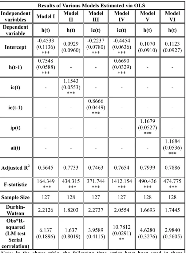
comparison of these three models altogether would allow us to determine whether the call, the put, or the average implied volatility value would be a better forecast. The estimation results for the proposed econometric models have been summarized in Table 4 below.

Table 4. Information Content of the Implied Volatility: Least Squares Estimates

Results of Various Models Estimated via OLS Independent

variables Model I Model II Model III Model IV Model V Model VI Dependent

variable h(t) h(t) ic(t) ic(t) h(t) h(t)

Intercept (0.1136) -0.4533 *** 0.0929 (0.0960) -0.2237 (0.0780) *** -0.4454 (0.0636) *** 0.1070 (0.0910) (0.0927) 0.1123 h(t-1) (0.0588) 0.7548 *** - - 0.6690 (0.0329) *** - - ic(t) - (0.0553) 1.1543 *** - - - - ic(t-1) - - (0.0449) 0.8666 *** - - - ip(t) - - - - (0.0527) 1.1679 *** - ai(t) - - - (0.0536) 1.1684 *** Adjusted R2 0.5645 0.7733 0.7463 0.7654 0.7939 0.7886 F-statistic 164.349 _*** 434.315 _*** 371.744 _*** 1412.154 _*** 490.436 _*** 474.775 _*** Sample Size 127 128 127 127 128 128 Durbin-Watson 2.2126 1.8203 2.2737 2.0554 1.6693 1.7445 Obs*R-squared (LM test Serial correlation) 6.137 (0.1896) (0.8019) 1.637 (0.4115) 3.9589 10.7812 (0.0291) ** 4.6280 (0.3276) (0.5605) 2.9840

Note: In the above table, the following time series have been used in these

estimations: The ex-post realized volatility (ht) calculated as the standard

deviation of the average monthly of the S&P 500 Index return over the life of the index option, and its first lag (ht-1), call option implied volatility(i_tc), put option

implied volatility( p t

i ), average implied volatility(aiv ). There are 128 monthly _t

observations in full sample, but including the lagged variables may cause decline in the sample size. There are 6 models reported in the table which utilize following regression equations:

Model I) ht = α0+ α1ht−1 + εt Model II) _{0 1} c t t t h = α + αi +ε Model III) itc= α0+ α1 1itc− +εt Model IV) itc = α0+ α1ht−1+εt Model V) ht =

α α

ε

Model VI) ht = α α₀+ aaivt+εt

Numbers in parenthesis are standard deviations for the coefficients and P values for chi-squared test statistic for serial correlation test. Stars denote the significance of various types. *** means significant at 0.01 level, ** shows significance in 0.05 level, * indicates significance at 0.1 level and finally no stars means insignificance or failure of the rejection in that test. In the table, F-statistic is the value we rely on in testing overall significance of the model. stars in F-statistic part has similar meaning as in coefficient significance tests and serial correlation tests

As mentioned by Granger and Poon (2003), the regression based methodology for estimating the information content of the implied forecast entails regressing the implied on the forecasts, as in the second, fifth and sixth models. The prediction is unbiased only if the intercept term is zero and the coefficient is equal to one.

The Table 4 indicates that in the first model (ht = α0+ α1ht−1 + ), εt intercept term and coefficient of lagged realized v volatility are significant if we look at the t-statistic. F-statistic of the model also shows that model is overall significant. The R2 _{seems to be moderate in this model. Further, presence of first} order autocorrelation is in inconclusive area by Durbin Watson test since the statistic is between upper and lower bounds for rejection. Therefore, we cannot comment on presence of first order serial correlation. Moreover, we cannot also detect higher order serial correlation by LM test.

In Second model, coefficient of the intercept term is insignificant and other coefficient is significant on 0.01 confidence level. The Model II is also overall significant since F-statistic is high enough. We can observe a higher adjusted R2 value. This may be interpreted, as an evident proof of the superior power of the implied volatility over the future realized volatility as compared to the historical volatility. Moreover, Durbin Watson statistic appears to be higher than the upper bound for this statistic. Thus, it falls in rejection region. Again, from the LM test we cannot reject the null hypothesis of no higher order serial correlation.

Coefficients in the third model are all individually significant as there are jointly significant. Further, autocorrelation tests appear to be as good as in significance tests. Durbin Watson-statistic does not show that the first order serial correlation is rejected in the border of tests statistic and LM test does not indicate higher order serial correlations in residuals of the model.

Fourth model is also overall significant with individually significant coefficients. Though Durbin-Watson does not indicate first order serial correlation in residuals, LM test demonstrates evidence on existence of higher order serial correlation in residuals of the model.

Fifth and sixth model contains one insignificant coefficient, intercept term, and one significant parameter, coefficient of regressor. Models are again significant. We can observe highest adjusted R-square values among all models. We cannot also find presence of any serial correlation structure both first order and higher orders.

In order to explain slightly higher values of implied put volatility from the implied call, Christensen and Hansen (2002) mention the suggestion provided by Harvey and Whaley (1991; 1992), which implies that the slightly higher values might emerge from the pressure of buying put options. It stems from the fact that buying index put options is a convenient and inexpensive means for portfolio insurance. Despite this general acknowledgement, the most influential studies use the call implied volatility information content. Our results reveal a more interesting fact.

Since the call and put implied volatilities are so close, we assessed an alternative model, which is estimating the sixth model with including an average of the call and put implied variables. When we compare the sixth model, a slight improvement in adjusted R-square value is detected. Furthermore, when we compare the fourth, fifth and the sixth models, with the aim of comparing the relative information content of the call and put implied volatility in explaining the future volatility, the results clarified that put options are more appropriate for such information content and forecast performance measures.

4.2. Forecast Performance

From the regression analysis, it has been concluded that the put implied volatility is a better forecast of the future realized volatility. We need to check this posit by evaluating the forecast performances of three relative models. The three econometric models, namely model II (ht =

α α

ε

(_{ht =}

_{α α}

_ε

1

0 t

t aiv t

h = α α+ +ε ) have been compared with regard to their one-step ahead, i.e. static, forecast performances. In other words, we calculated whether the put implied, call implied or the average implied have a higher forecast performance over the future realized volatility series.

Table 5. Comparison of Forecast Performances Forecasts: Implied Call

Volatility Average Implied Volatility Put Implied Volatility Root Mean Squared Error 0.2479 0.2394 0.2364

Mean Absolute Error 0.1822 0.1776 0.1796

Mean Absolute Percentage Error 12.776 12.159 12.009 Theil Inequality Coefficient 0.0645 0.0623 0.0615

Bias Proportion 0.0000 0.0000 0.0000

Variance Proportion 0.0635 0.0587 0.0571

Covariance Proportion 0.9364 0.9412 0.9428

Note: The forecast by call implied volatility represents the forecast of the model II

(ht =

α α

ε

forecast of the model and model VI (ht = α α0+ 1aivt+εt), and the forecast by average implied volatility represents the forecast of the Model V (_{ht =}

_{α α}

_ε

From the model selection criteria as well as the significance of the models, the put implied volatility should have superior forecast performance. Indeed when we look at the comparative forecast performances in Table 4, we can clearly confirm this deduction. When we look at the root mean squared error and the mean absolute error values, the smallest error, thus better forecasting ability belongs to the error, the better the forecasting ability of that model according to that criterion.

In Table 5 above, the comparative one-step ahead forecast performances could be seen. The inequality coefficient denotes the fit, with zero indicating a

perfect fit. The bias proportion indicates how far the forecast mean from the realized mean, the variance indicates how far the forecast variation from the realized variation, and covariance proportion shows the unsystematic forecasting error proportion.

While among the one-step ahead forecasts, the put implied volatility has the highest forecast ability, the low bias and variance proportions indicate the goodness of forecast.

We want to expand this strong hypothesis by investigating whether the long-term, the medium-term and short-term volatility have different information content and forecasting ability. For this purpose, we adapted the wavelet multi-scale decomposition method. We want to filter out the different components of the series without distorting the data.

For this purpose, different techniques are available. We should consider that the method should produce robust empirical results to explain the time varying properties of especially persistent and serially correlated series. In finance, it is common to investigate issues of filtering in the frequency domain especially for time series, since this type of analysis more naturally lends itself to the decomposition of a time series into sums of periodic patterns.

Still, various filtering methods, starting from deterministic detrending to Beveridge-Nelson decomposition and Hodrick Prescott filter all have shortcomings. The deterministic de-trending assumes uncorrelated trend and cycles and Beveridge-Nelson is an equivalent expression of the infinite moving average.

Moreover, Hodrick Prescott filter results depend on the choice of λ parameter, which makes the resulting cyclical component and its statistical properties highly sensitive to this choice. As one of the latter tools, the Baxter-King filter is a band-pass filter, which is in reality a centered moving average with symmetric weights. However, it has been criticized because it induces spurious dynamics in the cyclical component (Jorda, 2010). Briefly, those earlier filtering methods are all subject to restrictive assumptions that make them rather inappropriate for analyzing the persistent financial time series data.

CHAPTER 5

WAVELET DECOMPOSITION

Wavelet method is essentially a novel filtering technique. It allows us to account for the nonlinearity and other erratic features present in financial data without any manipulation of characteristic features present in financial series (e.g. spillovers, clustering, heteroscedasticity etc.). Conventional methods have been described as rather inappropriate to handle most financial and economic time series data (Granger and Poon, 2003).

Recently, wavelet decomposition has been introduced in economic and financial analysis, and the literature on the subject has been expanding rapidly. Ramsey and Zhang (1997) use the wavelet decomposition to analyze the dynamics of the foreign exchange rates. They conclude that wavelet analysis is able to capture a variety of properties of non-stationary time series. Ramsey and Lampart (1998) decompose economic variables across several wavelet scales in order to identify different relationships between money and income, and between consumption

and income. Then, Gencay et al. (2001) demonstrate that wavelet filtering is an appropriate tool to deal with the nonstationary and time-varying features of financial time series.

In addition, a variety of academic studies conclude that conventional time series methods focus exclusively on a time series at a given scale and they assume an unconditional universal time scale for the risk, i.e. volatility. Such studies include Ding et al. (1993), Andersen and Bollerslev (1997), Lobato and Savin (1998), and Dacorogna et al. (2001) and Gencay et al. (2002, 2004).

In that regard, the previous studies of Gencay et al. (2001, 2002, 2004, 2005, 2009 and 2010) strongly emphasize the heterogeneous characteristics of volatility. Gencay et al. (2005) particularly emphasize the nonstationarity and asymmetry of volatility by implementing wavelet analysis to financial data. According to them, the volatility features imply that low-frequency volatility becomes effective in the long-run, and vice versa. Gencay et al. further underline that nonstationarity of different moments of financial time prohibit and nullify the popular model assumptions such as Wiener Process etc.

Essentially, wavelet analysis decomposes a series into a set of trend (approximation) and detail (cyclical) components. The detail components cover different frequency bands, which are effective for different periods. The periods correspond to short-run, medium-run, long-run depending on their time span. The levels are described as the decomposition of the series with high-pass and low-pas filters, which can preserve orthogonality. It means that levels do not contain information about each other and the summations of the levels recreate the original

series. It is important to remember that market players have different investment or risk exposure horizons, and corresponding to their specific goals for each term, take different positions in the short-run, medium-run and long-run. Accordingly, wavelet analysis offers a complementary time and frequency domain analysis simultaneously.

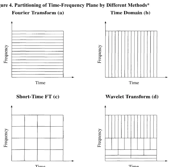
The classical Fourier transform has been a powerful tool for modern time series analysis and widely used to transform series from time domain to frequency domain. It is a traditional filtering technique used to analyze the frequency structure of time series. However, it poses challenges and constraints. In Fourier analysis, a series is transformed onto a set of orthogonal components, which are stationary sine and cosine functions. Hence, it is described as inadequate when dealing with financial time series.

Analogous to the orthogonal components in Fourier transform, wavelets are any wave functions that are localized in time and frequency domains. They are able to capture dynamic properties of time series. In fact, the orthogonal components retrieved via wavelet decomposition describe properties both at time and frequency plane, thereby extracting the transient patterns of idiosyncratic time series.

Figure 4. Partitioning of Time-Frequency Plane by Different Methods*

*Adapted from “An Introduction to Wavelets and Other Filtering Methods in Finance and Economics” by R. Gencay, F. Selcuk and B. Whitcher, 2002, p. 98. Copyright 2002. by Academic Press.

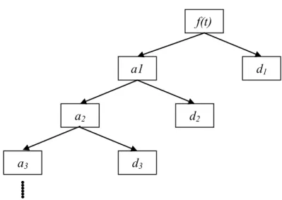
In wavelet analysis, the function f(t) is translated and dilated onto the father

( )t

ϕ and mother wavelets ψ( )t . The mother wavelet functions ψ define the details, they have unit energy and zero mean, i.e. integral is zero; it is chosen with a compact support to obtain localization in space. In addition, the father wavelet functions φ define scaling, i.e. approximations and its integral is one.

( )t dt 0

ψ =

Mother wavelets are described as the translation functions, or high-pass filters. In contrast, the father wavelets are dilation functions or low-pass filters, such that: 2 , ( ) 2 j (2 j ) j k t t k ψ ₌ − ψ − _{− with j k Z, ∈ =}

{

}

{

}

And the wavelet representation of the function f(t) can be described as:

, , , , 1, 1, , , 1, 1,

( ) J k J k( ) J k J k( ) J k J k( ) J k J k( ) ... k k( )

k k k k k

f t =

∑

∑

∑

∑

∑

J is the level of decomposition and k ranges from 1 to the number of

coefficients in each specific component. The coefficients a dJ k, , J k, ,... are the

wavelet transform coefficients given by the following projections:

( ) ( )

∫

∫

( ) ( )

That is, wavelet transform decomposes or translates function into orthogonal components at different scales. For the function f(t), the wavelet multi-resolution in the time-frequency domain corresponds to the following:

f(t) = AJ(t) + DJ(t) + ……. + D2(t) + D1(t) where , , ( ) ( ) J J k J k k A t =

∑

∑

∑

∑

Aj(t) are defined as the smooth approximations while Dj(t) are known as the detail levels. In this case, n=2J _{measures the scale and it is called as the dilation}

factor. Then, the discrete wavelet transform can be described as:

∫

Also, the inverse wavelet transform can be described as:

∑ ∑

=

w

t

t

f

(

)

~

ψ

(

)

The discrete wavelet transform (DWT) is defined as a mathematical tool that projects a time series onto collection of components. These components capture information from the time series at different frequencies at distinct times. (Gencay et al., 2010) The DWT has the advantage of time resolution by using basis functions that are local in time. However, the choice of a wavelet basis is an important issue in DWT; in that case the length of the data should be taken into account.

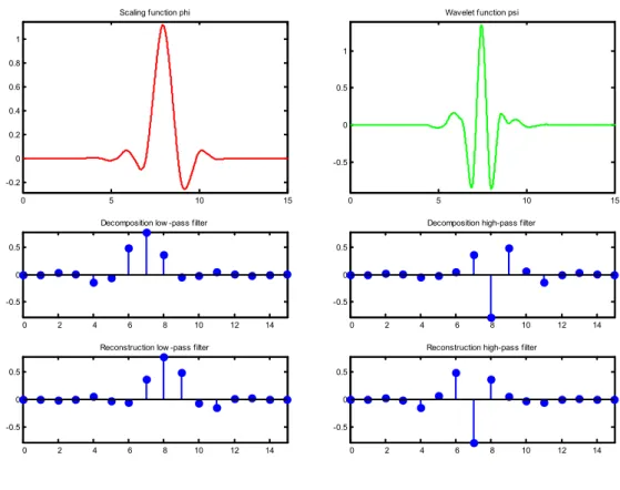
Specifically, in empirical analysis four types of orthogonal wavelets; namely haar, daubechies, symlet and coiflet wavelets are present. In order to preserve orthogonality in our estimations and considering the sample length and the time series features of the volatility, the Symlet-8 wavelet family has been chosen. The Figure 13 below shows the Symlet high-pass, and low-pass filter properties.

The wavelet decompositions of realized and implied volatility series are performed by using the wavelet basis Symlet 8 (Daubechies, 1992). Since the volatility series consist of 128 observations and the length of Symlet 8 basis is 16, using the general criterion:

( ) (

)

(

)

( )

2

log length x lwave Level log     =  − _

Here, Level denotes maximum level of decomposition; length(x) is the length of the series; lwave is the length of the wavelet basis.

Figure 6. Symlet-8 Wavelet Family: Wavelet and Scaling Functions 0 5 10 15 -0.2 0 0.2 0.4 0.6 0.8 1

Scaling function phi

0 5 10 15

-0.5 0 0.5 1

Wavelet function psi

0 2 4 6 8 10 12 14 -0.5

0 0.5

Decomposition low -pass filter

0 2 4 6 8 10 12 14 -0.5

0 0.5

Reconstruction low -pass filter

0 2 4 6 8 10 12 14 -0.5

0 0.5

Decomposition high-pass filter

0 2 4 6 8 10 12 14 -0.5

0 0.5

Reconstruction high-pass filter

The calculation for the optimum decomposition level indicates that J=3 levels. The original time series can be reconstructed by summing all three detail levels plus the approximation level.

Since lower frequencies will prevail for a longer period, the corresponding scales and their time domain characterizations are described in the Table below. It is interpreted as the observed magnitudes on the first detail scale have higher frequency values, but they will be observed for a shorter period, e.g. up to three months.

Table 6. Time Scales

Scale Frequency

Detail Scale 1 (Dj=1) Up to three months Detail Scale 2 (Dj=2) Up to six months Detail Scale 3 (Dj=3) Up to a year Approximation (Aj=3) Over a year

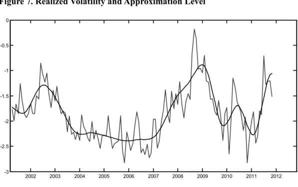
The Figures 7-12 below show the approximation and the detail levels of the S&P 500 Index realized volatility graphically. The wavelet decomposition analysis has been implemented via MATLAB Software.

It should be noted that since the put implied volatility is found to be a superior forecast of the future realized volatility, in wavelet analysis, the scale-by-scale relationship between the put implied and the realized volatility has been estimated. The results confirm different characteristics and explanatory power of the different components, e.g. lower-frequency and higher period components and so on, of put implied over the future realized volatility.

Figure 7. Realized Volatility and Approximation Level

2002 2003 2004 2005 2006 2007 2008 2009 2010 2011 2012 -3 -2.5 -2 -1.5 -1 -0.5 0