Human motion control using inverse kinematics

HUMAN MOTION CONTROL USING

INVERSE KINEMATICS

a thesis

submitted to the department of computer engineering

and the institute of engineering and science

of bilkent university

in partial fulfillment of the requirements

for the degree of

master of science

By

Aydemir MEM˙IS¸O ˇ

GLU

August, 2003

I certify that I have read this thesis and that in my opinion it is fully adequate, in scope and in quality, as a thesis for the degree of Master of Science.

Prof. Dr. B¨ulent ¨Ozg¨u¸c (Supervisor)

I certify that I have read this thesis and that in my opinion it is fully adequate, in scope and in quality, as a thesis for the degree of Master of Science.

Assist. Prof. Dr. U˘gur G¨ud¨ukbay (Co-supervisor)

I certify that I have read this thesis and that in my opinion it is fully adequate, in scope and in quality, as a thesis for the degree of Master of Science.

Prof. Dr. ¨Ozg¨ur Ulusoy

Approved for the Institute of Engineering and Science:

Prof. Dr. Mehmet Baray Director of the Institute

ABSTRACT

HUMAN MOTION CONTROL USING

INVERSE KINEMATICS

Aydemir MEM˙IS¸O ˇ

GLU

M.S. in Computer Engineering

Supervisors: Prof. Dr. B¨ulent ¨

Ozg¨u¸c

and Assist. Prof. Dr. U˘gur G¨ud¨ukbay

August, 2003

Articulated figure animation receives particular attention of the computer graph-ics society. The techniques for animation of articulated figures range from simple interpolation between keyframes methods to motion-capture techniques. One of these techniques, inverse kinematics, which is adopted from robotics, provides the animator the ability to specify a large quantity of motion parameters that results with realistic animations. This study presents an interactive hierarchical motion control system used for the animation of human figure locomotion. We aimed to develop an articulated figure animation system that creates movements , like goal-directed motion and walking by using motion control techniques at different levels. Inverse Kinematics using Analytical Methods (IKAN) software, which was developed at the University of Pennsylvania, is utilized for controlling the motion of the articulated body using inverse kinematics.

Keywords: kinematics, inverse kinematics, articulated figure, motion control,

¨

OZET

TERS K˙INEMAT˙IK Y ¨

ONTEM˙I KULLANILARAK ˙INSAN

HAREKET˙IN˙IN KONTROL ¨

U

Aydemir MEM˙IS¸O ˇ

GLU

Bilgisayar M¨uhendisli˘gi B¨ol¨um¨u, Y¨uksek Lisans

Tez Y¨oneticileri: Prof. Dr. B¨ulent ¨

Ozg¨u¸c

ve Yrd. Do¸c. Dr. U˘gur G¨ud¨ukbay

A˘gustos, 2003

Eklemli v¨ucutların animasyonu bilgisayar grafi˘gi alanında en fazla ilgi ¸ceken konulardan biridir. Eklemli v¨ucutların animasyonu i¸cin geli¸stirilen teknikler, anahtar resimler arasında ara de˘ger kestirimi metodlarından hareket yakalama tekniklerine kadar geni¸s bir yelpaze olu¸sturmaktadır. Bu tekniklerden biri olan ve robotbilimden uyarlanan ters kinematik y¨ontemi, canlandırıcıya bir¸cok hareket parametresini tanımlayabilme imkanı vererek ger¸cek¸ci bir animasyona olanak sa˘glamaktadır. Bu ¸calı¸smada, insan v¨ucudunun y¨ur¨ume hareketi i¸cin kul-lanılan etkile¸simli, hiyerar¸sik bir hareket kontrol sistemi anlatılmaktadır. Ayrıca, ¸calı¸sma kapsamında, hedefe y¨onelik hareket ve y¨ur¨ume gibi de˘gi¸sik seviyelerde hareket kontrol teknikleri kullanılarak, eklemli v¨ucut canlandırması yapan bir sistem geli¸stirilmi¸stir. Eklemli v¨ucudun hareketini ters kinematik y¨ontemi kulla-narak kontrol etmek i¸cin, Pennsylvania ¨Universitesi’nde geli¸stirilen IKAN yazılım paketinden yararlanılmı¸stır.

Anahtar kelimeler: kinematik, ters kinematik, eklemli v¨ucut, hareket kontrol¨u,

ACKNOWLEDGMENTS

I am gratefully thankful to my supervisors Prof. Dr. B¨ulent ¨Ozg¨u¸c and As-sist. Prof. Dr. U˘gur G¨ud¨ukbay for their supervision, guidance, and suggestions throughout the development of this thesis.

I would also like to give special thanks to my thesis committee member Prof. Dr. ¨Ozg¨ur Ulusoy for his valuable comments.

Contents

1 INTRODUCTION 1

1.1 Organization of the Thesis . . . 3

2 RELATED WORK 5 2.1 Body Models . . . 5

2.1.1 The H-Anim 1.1 Specification . . . 7

2.2 Kinematics . . . 10 2.2.1 Forward Kinematics . . . 10 2.2.2 Inverse Kinematics . . . 12 2.2.3 Discussion . . . 15 2.3 Dynamics . . . 16 2.3.1 Forward Dynamics . . . 16 2.3.2 Inverse Dynamics . . . 17 2.3.3 Discussion . . . 18 2.4 Motion Capture . . . 18

2.4.1 Discussion . . . 19

2.5 Motion Control . . . 19

2.5.1 Interpolation Control . . . 20

3 ARTICULATED FIGURE MODELING 23

3.1 XML Based Model . . . 23

4 MOTION CONTROL 29

4.1 Low-Level Control of Motion . . . 30

4.2 Human Walking Behaviour . . . 37

5 IKAN 44

5.1 Motion of the Skeleton . . . 44

5.2 Implementation Details . . . 47 6 EXPERIMENTAL RESULTS 50 6.1 Visual Results . . . 50 6.2 Performance Analysis . . . 58 7 CONCLUSION 59 APPENDICES 61

A.1 Document Type Definition (DTD) of Human Model . . . 61

A.2 XML Formatted Data of Human Model . . . 62

B CLASS DIAGRAMS 65 B.1 Hbody Package . . . 65

B.2 HBodyIK Package . . . 70

B.3 Curve Package . . . 73

C THE SYSTEM AT WORK 77 C.1 Overview . . . 77

C.1.1 The Main Menu . . . 79

C.1.2 The Motion Control Toolbox . . . 79

C.1.3 The Keyframe Editor . . . 80

C.1.4 The Viewing Area . . . 82

List of Figures

2.1 A manipulator with three degrees of freedom (reprinted from [41]). 7

2.2 The H-Anim Specification 1.1 hierarchy (reproduced from [36]). . 9

2.3 The Denavit-Hartenberg Notation (adopted from [16]). . . 11

3.1 A portion of humanoid data in XML format. . . 24

3.2 Level of articulations: a) level of zero, b) level of one, c) level of two, and d) level of three. . . 25

3.3 Left and top view of the skeleton. . . 26

3.4 UML class diagram of the Hbody package. . . 27

4.1 A piecewise continuous cubic-spline interpolation of n + 1 control points. . . 31

4.2 Parametric point function P (u) for a Hermite-spline section. . . . 32

4.3 Parametric point function P (u) for a Cardinal-spline section. . . . 32

4.5 Intervals of equal parametric length (outlined arrowheads) do not correspond to equal intervals of arclength (black arrowheads)

(reprinted from [41]). . . 36

4.6 Locomotion cycle for bipedal walking (adopted from [32]). . . 38

4.7 Walking gaits: (a) compass gait, (b) pelvic tilt, (c) plantar flexion, (d) pelvic rotation, (e) stance leg inflexion, and (f) lateral pelvic displacement (reprinted from [41]). . . 40

4.8 The velocity curve of a) left ankle and b) right ankle. . . 43

4.9 The distance curve of a) left ankle and b) right ankle. . . 43

5.1 Example arm showing the selection of projection and positive axis (reprinted from [15]). . . 46

5.2 UML class diagram for IKAN classes that is used in our system. 47 5.3 The joint orientations for the end-effector positioning for the right arm and the left foot. . . 49

6.1 Front view of the walking articulated figure. . . 51

6.2 Side view of the walking articulated figure. . . 52

6.3 Top view of the walking articulated figure. . . 53

6.4 Skinned human model walking behavior. . . 54

6.5 Goal-directed motion of the arm of the articulated figure. . . 56

6.6 Goal-directed motion of the leg of the articulated figure. . . 57

C.2 The motion control toolbox . . . 80

C.3 The keyframe editor . . . 81

List of Tables

B.1 Humanoid attributes . . . 65 B.2 Humanoid methods . . . 66 B.3 Node attributes . . . 66 B.4 Node methods . . . 67 B.5 Joint attributes . . . 67 B.6 Joint methods . . . 68 B.7 Segment attributes . . . 68 B.8 Segment methods . . . 68 B.9 Site methods . . . 69 B.10 HALChain attributes . . . 70 B.11 HALChain methods . . . 70 B.12 Arm attributes . . . 71 B.13 Arm methods . . . 71 B.14 Leg attributes . . . 72

B.15 Leg methods . . . 72 B.16 Curve Attributes . . . 73 B.17 Curve Methods . . . 74 B.18 CubicSpline Attributes . . . 74 B.19 CubicSpline Methods . . . 75 B.20 CardinalSpline Attributes . . . 75 B.21 CardinalSpline Methods . . . 75 B.22 Line Methods . . . 76

Chapter 1

INTRODUCTION

Today, computer graphics has reached to a point where computer generated images has become almost indistinguishable from the real scenes. Nevertheless, animating the objects in a realistic manner is still difficult, particularly as object models become more complex. As a result, the specification and control of motion for computer animation became one of the principal areas of research within computer graphics community.

One area, which receives particular attention, is figure animation. Research in this area focuses on generating realistic articulated figures, and designing and controlling their movements. There are many applications in which virtual humans are involved; from special effects in film industry to virtual reality and video games. However, the human motion created by the artists is not always realistic and the reasons that prevent the realism increase the difficulty of the task.

During fifteen years period in the study of human motion, many techniques based on kinematics, dynamics, biomechanics, and robotics was developed by the researchers. The task was very complicated but the interest for this area has never decreased. It was used in several applications, such as robotics, art,

entertainment, education, and biomedical researches and the type of application in which walking motions is used, determined the constraints that the model has to solve. On the one hand, video games or virtual reality applications require the minimization of the ratio between the computation cost and capabilities of the model. However, for biomedical researches, the important constraint is that the model must be realistic and the animation of the model should obey the physical laws. Therefore, the models are designed and animated according to the specific application area in which they are applied. It is possible to classify the animation of the models into three main groups:

• procedural methods based on kinematic animation, • dynamic methods based on dynamics constraints, and • motion capture methods.

In this study, we aimed to develop an articulated figure animation system that creates movements using low-level motion control techniques, goal-oriented ani-mation, and high-level motion control techniques like walking. Inverse kinematic techniques were used mainly for creating new movements.

The articulated figure is modelled using Extensible Markup Language (XML) data format. The hierarchy of joints and segments of human skeleton and their naming conventions are adopted from the Humanoid Animation (H-Anim) 1.1 Specification. Besides, the elements of the XML data is organized as they are corresponding to the nodes of the H-Anim structure. However, since the whole hierarchy defined in H-Anim 1.1 Specification is redundant for our system, a simplified version of the hierarchy is implemented. The resulting framework is suitable for modeling various articulated structures like humans, robots and etc.

This study solves the motion controlling of the articulated figure by a low-level control of motion using kinematic methods. We characterized this low-low-level

motion control by using spline-driven animation techniques. Besides, a high-level walking system, which is based on low-level techniques, is introduced.

Smooth motions are generated using spline-driven animation techniques. A class of cubic splines, Cardinal splines, is preferred due to their less calculation and memory requirements and capability for local control over the shape. Cardi-nal splines are used in generating the paths for pelvis, ankle, and wrist motions, which are considered as position curves. In addition, a velocity curve or distance curve for each object is produced that enables us changing the behavior of the motion. Arclength parameterization of the spline method is used in order to determine the position of each object along the position curve at each frame. All of these are the components of our low-level animation system.

By using this low-level system, a high-level motion mechanism for walking is implemented. In walking motion, the limb trajectories and joint angles are computed automatically using some parameters like locomotion velocity, size of walking step, the time elapsed during double-support, rotation, tilt, and lateral displacement of pelvis.

Inverse kinematics is heavily used in our system. Inverse Kinematics

us-ing Analytical Methods (IKAN) software package, which was developed at the

University of Pennsylvania, is used to compute the desired limb positions.

1.1

Organization of the Thesis

The thesis is organized as follows: Chapter 2 reviews computer animation tech-niques and discusses their applicability in the articulated figure animation. In Chapter 3, the articulated figure modeling approach that is used in our study is discussed. Chapter 4 focuses on low-level and high-level motion control tech-niques in our system. Chapter 5 deals with the capabilities of IKAN software,

and the usage of this tool in our study. Chapter 6 gives the performance re-sults of the implementation. Chapter 7 presents conclusions and future research areas. In Appendix A, the human model in XML format that is used in our system is described. Appendix B focuses on class diagrams and implementation details. Lastly, Appendix C gives information about the application and its user interface.

Chapter 2

RELATED WORK

This chapter summarizes the computer animation techniques for articulated fig-ure animation in general. It depicts the human figfig-ure modeling techniques and the advantages and disadvantages of basic motion control techniques for figure animation. Moreover, a summary is given about the background work in human walking.

The work involved in the animation of human motion, could simply be divided into three major steps: modeling the basic structure (skeleton), motion of the

skeleton, and creation of the body appearance. In this chapter, related work

including the figure modeling and control of the motion of the skeleton will be given.

2.1

Body Models

One of the main problem in human character animation is the model structure. What kind of model we will use. It is clear that building a physically realistic model as possible as a real human character is the main goal. The ideal, computer generated character should consider the accurate positioning of human limbs

during motion, the skin where muscles and tissue deforms during the movement, expressive facial expressions, realistic modeling of hair, and etc. However these are all research topics in their own right.

The basic approach to this problem is to start with structuring the skeleton part of human and then, adding the muscle, skin, hair and other layers to that structure. Skeleton layer, muscle layer, and skin layer are the most common ones. This layered modeling technique is heavily used in human modeling field of computer graphics [14]. In that approach, motion control techniques are just applied on the skeleton layer and this simplifies the challenging work because there is no need to think about the details of the model.

Modeling the articulated skeleton is the trivial part of the human body model-ing. Skeleton can be represented as a collection of simple rigid objects connected together by joints. The joints are arranged in a hierarchical structure to model human like structures. These models, called articulated bodies, can be more or less complex. The number and the hierarchy of joints and limbs and the degrees of freedoms (DOF) of joints determine the complexity of model. Degree of free-dom of a joint is the independent position variables that are necessary to specify the state of the joint (see Figure 2.1). The joints can rotate in one, two, or three orthogonal directions. The number of these orthogonal directions determines DOF of a joint. A human skeleton may have many DOFs. However, when the number of DOFs increases, the mathematics of the structure, which is used for controlling the joints, becomes more complex. Besides, some restrictions such as limiting the rotation angle of that in each of the rotation directions, provide more simplified solutions.

Figure 2.1: A manipulator with three degrees of freedom (reprinted from [41]).

2.1.1

The H-Anim 1.1 Specification

Modeling the basic structure of the articulated figure is the trivial part of the challenging work. However, a challenge arises when human model needs to be in-terchangeable. A standard should exist among the people who deal with human modeling, so that interchangeable humanoids can be created. The Humanoid Animation Working Group of Web3D Consortium developed the Humanoid

An-imation (H-Anim) specification for this purpose. They specified the way of

defin-ing humanoid forms and behaviors in standard Extensible 3D Graphics/Virtual Reality Modeling Language (X3D/VRML). In the scope of their flexibility goal, no assumptions are made about the types of application that will use humanoids. Their simplicity goal guided them to focus specifically on humanoids, instead of trying to deal with arbitrary articulated figures.

Human body consists of a number of segments (such as the forearm, hand, foot) that are connected to each other by joints (such as the elbow, wrist and ankle). The H-Anim structure contains a set of nodes to represent the hu-man body. The nodes are Joint, Segment, Site, Displacer, and Huhu-manoid.

Joint nodes represent the joints of human body and they are arranged in a strictly defined hierarchy. They may contain other Joint and Segment nodes. Segment nodes represent a portion of the body connected to a joint. They may contain Site and Displacer nodes. Site nodes are used for placing cloth and jewelry. Besides, Site nodes can be used as end-effectors for inverse kinematics applications. Displacer nodes are simply grouping nodes, allowing the program-mer to identify a collection of vertices as belonging to a functional group for ease of manipulation. Humanoid node stores information about the model. It acts as a root node for the body hierarchy and stores all the references to Joint, Segment, and Site nodes. The basic structure of human body model is built by using these nodes in a H-Anim file. In addition, a H-Anim compliant human body is modeled “at rest” position. At that position, all the joint angles are zero and humanoid faces the +z direction, with +y being up and +x to the left of the humanoid according to right hand coordinate system. The complete body hierarchy with joints and their associated segments, and naming conventions for H-Anim Specification is given in Figure 2.2.

2.2

Kinematics

Kinematic methods, which originate from field of robotics, is one of the ap-proaches used in motion specification and control. Animation of the skeleton can be performed by changing the orientations of joints by time. Motion control is the management of the transformations of the joints by time. Kinematics is the study of motion by considering the position, velocity, and acceleration. It does not emphasize on the underlying forces that produces the motion. forward and inverse kinematics are the two main categories of kinematic animation.

2.2.1

Forward Kinematics

Although articulated figures are constructed from a few number of segments, we should deal with much number of degrees of freedoms. There are many motion parameters that should be controlled to have the desired effect on a simple character. Forward kinematics is the way of setting the such motion parameters, like position and orientation of skeleton, at specific times. By directly setting the rotations at joints, and giving a global transformation to the root joint, different poses can be handled. The motion of the end-effector (in the case of arm, the hand) is determined by indirect manipulations of transformations in root joint of skeleton, and rotations at shoulder and elbow joints. Mathematically, forward kinematics is expressed as

x = f (Θ) (2.1) That is, given Θ, derive x. In case of the leg, given the rotation angles of knee and hip, the position of the foot is calculated by using the positions and rotations of the hip and knee.

In order to work on the articulated figures, a matrix representation, which will define the rotation and orientations, should exist. Denavit and Hartenberg

were the first who developed a notation, called DH notation, to represent the matrix formulation for kinematics of articulated chains [16]. DH notation is a link based notation where each link is represented by four parameters; Θ, d, a, and α (see Figure 2.3). For a link, Θ is the joint angle, d is the distance from the origin, a is the offset distance, and α is the offset angle. The relations between the links are represented by 4 × 4 matrices.

Figure 2.3: The Denavit-Hartenberg Notation (adopted from [16]).

Moreover, Sims and Zeltzer [35] proposed a more intuitive method, called

axis-position (AP) representation. In this approach, the position of the joint,

the orientation of the joint and the pointers to joint’s child nodes are considered to represent the articulated figure.

In forward kinematics, after the orientation matrix of each joint is calculated, the final position of end-effector is found by multiplying the matrices in the same manner as computing graphics transformation hierarchies.

2.2.2

Inverse Kinematics

Inverse kinematics is a more high-level approach. It is sometimes called as “goal-directed motion”. Given the positions of end-effectors only, the inverse kinematics solves the position and orientation of all the joints in the hierarchy. Mathematically, it is expressed as

Θ = f−1_{(x) (2.2)}

That is, given x, derive Θ.

Inverse kinematics was mostly used in the robotics. The studies in this area are then adapted to the computer animation. Contrary to forward kinematics, inverse kinematics provides direct control over the movement of the end-effector. On the other hand the inverse kinematic problems are difficult to solve where, in forward kinematics, the solution is found easily by multiplying local transforma-tion matrices of joints in a hierarchical manner. The inverse kinematics problems are non-linear and for a given position x there may be more than one solution for Θ.

Mainly, there are two approaches to solve inverse kinematics problem:

Nu-merical and analytical methods.

2.2.2.1 Numerical Methods

The most common solution method for the non-linear problem stated in Equa-tion 2.2 is based on the linearizaEqua-tion of the problem by means of its current configuration [49]. When we linearize the problem the joint velocities and the end-effector velocity will be related by:

As it is denoted in the Equation 2.3, the relation is expressed by the Jacobian matrix:

J = δf

δΘ (2.4)

This matrix relates the changes in the joint variables (δf ) with the changes in the position of the end-effector (δΘ) in an m × n manner, where m is the joint variables count and n is the dimensions of the end-effector vector.

When we invert the Equation 2.3 we reach the formula:

˙Θ = J−1_{(Θ) ˙x (2.5)}

So it is clear that given the inverse of Jacobian, computing the changes in the joint variables due to the change in the end-effector position is trivial. We can develop an iterative algorithm for the solution of this inverse kinematic problem. Each iteration computes the ˙x value by using actual and goal position vectors of end-effector. The iteration continues till the goal position of the end-effector is reached. However, in order to compute the joint velocities, ( ˙Θ) we must find the

J(Θ) value for each iteration.

At each iteration, we are trying to determine the end-effector frame move-ments with respect to joint variable changes. The frame movemove-ments are denoted by the columns of the Jacobian matrix J, and for a given joint variable vector (Θ), determined by the position (P(Θ)) and orientation (O(Θ)). So, the Jacobian column entry for the ith joint is:

Ji =                δPx/δΘi δPy/δΘi δPz/δΘi δQx/δΘi δQy/δΘi δQz/δΘi                (2.6)

These entries can be calculated as follows: Every joint i in the system trans-lates along or rotates above a local axis ui. If we denote the transformation

matrix between local frames and world frames as Mi, the normalized

transfor-mation of the local joint axis will be:

axisi = uiMi (2.7)

By using Equation 2.7, we can calculate the Jacobian entry either for a translating joint by: Ji =          [axisi]T 0 0 0          (2.8)

or for a rotating entry by:

Ji =   [(p − ji) × axisi]T (axisi)T   _(2.9)

At that point, we want to state that linearization solution makes an assump-tion that the Jacobian matrix is invertible (both square and non-singular), while this is not the case in general. In case of redundancy and singularities of the ma-nipulator, the problem is more difficult to solve and new approaches are needed.

2.2.2.2 Analytical Methods

In contrast with the numerical methods, analytical methods find solutions in most cases. We can classify the analytical methods into two groups; closed-form or algebraic elimination based methods [15]. Closed-closed-form method specifies the joint variables by a set of closed-form equations and generally applies to six degree of freedom systems with special kinematic structure. On the other hand, in algebraic elimination based method, the joint variables are denoted by

a system of multivariable polynomial equations. Generally, the degree of these polynomials are greater than four. That is why, algebraic elimination methods still require numerical solutions. In general, analytical methods are more likely than the numerical ones because analytical methods find all solutions and are faster and more reliable.

2.2.3

Discussion

The main advantages of kinematics are as follows: Firstly the motion quality is based on the model and the animator’s capability. The second advantage is the low cost of the computations. On the other hand in both kinematic methods, the animator still spends lots of time in order to produce movement. In other words, the methods can not produce movement in a dynamic manner by means of the physical laws as in the real world. Moreover, the interpolation process of the algorithms leads to loss of realism in the animation.

When we reviewed the literature we saw that Chadwick et al. had used inverse kinematics in creating keyframes [14]. Welman investigates the inverse kinemat-ics in detail and describes the constrained inverse kinematic figure manipulation techniques [42]. Badler et al. also proposed an inverse kinematic algorithm in order to constraint the positions of the body parts during animation [2]. In addi-tion, Girard and Maciejewski [18] and Sims and Zeltzer [35] generated leg motion by means of inverse kinematics. Their systems are composed of two stages: In the first stage, foot trajectories are specified, and in the second one, the inverse kinematic algorithm computes the leg joint angles during movement of the feet.

2.3

Dynamics

Physical laws heavily affect the realism of a walking motion. In this sense, dynamics approaches may be used for animating walking models. But these approaches require more physical constraints such as center of mass, total mass and inertia. Fundamental principles of dynamics are originated from Newton’s laws and can be stated by following:

f = m × ¨X (2.10) where f represents the force applied to an object, m is its mass and ¨X denotes the

second derivative of the position vector X with respect to time. The dynamics methods can be classified in two main parts: the forward dynamics and the

inverse dynamics.

2.3.1

Forward Dynamics

Basically, forward dynamics considers applying forces on the objects. These forces can be applied automatically or by the animator. The motion of the object is then computed by solving the equations of the motion for the object as a result of these forces. Wilhelm gives a brief summary of rigid body animation by means of forward dynamics methods [45]. Although the method works well with a rigid body, the simulation of articulated figures by forward dynamics is more complicated. Because, the equations of motion for articulated bodies must also handle the interaction between the body parts. This extension in the equation makes the control hardly difficult. Nevertheless, more than fifteen years ago, Virya system tried to simulate an articulated figure by forward dynamics methods [43]. This attempt was followed by many others [1, 46].

The main drawback of the forward dynamic simulation is that, not having an accurate control mechanism makes the method useful for the tasks in which initial values are known.

2.3.2

Inverse Dynamics

In the contrary, inverse dynamics is a goal oriented method in which forces needed for a motion are computed automatically. Although the inverse dynamics applications are rarely used in computer animation, Barzel and Barr [7] were the first users of the method. They generated a model composed of objets which are geometrically related. This relations are presented by constraints that are used to denote forces on a object. These forces animate the figure directed to a goal in which all the constraints are satisfied. The Manikin system proposed by Forsey and Wilhelm [17] also animated articulated model by means of inverse dynamics. The system computes the needed forces when a new goal position for the figure is specified. An other approach was introduced by Isaac and Cohen [24] which was called as Dynamo system and based on keyframed kinematics and inverse dynamics. This method is an example of combination of dynamic simulation and kinematic control. Ko also developed a real-time algorithm for animating human locomotion using inverse dynamics, balance and comfort control [26].

All the studies stated above describes the motion of a figure by considering geometric constraints. On the other hand, researchers developed some inverse dy-namics solutions based on non-geometric constraints. Brotman and Netravali [9], Girard [19] and Lee et al. [29] are some examples of these researchers.

2.3.3

Discussion

The composition of the anatomical knowledge with the inverse dynamics ap-proach generates more realistic motion. This composite system can also handle the interaction of the model with the environment. That is why, this method is useful for virtual reality applications. However, dynamic techniques are com-putationally costly than the kinematic techniques and hardly used in interactive animation tools.

Using purely a direct dynamics system or an inverse dynamics system has problems. To have the desired motion and use high level control, hybrid solutions should be applied. The need for the combination of forward and inverse dynamics is discussed in [30].

2.4

Motion Capture

Since dynamics simulation could not solve all animation problems, new ap-proaches were introduced. One of these methods animates virtual models by using human motion data generated by motion capture techniques. It is mainly used in the film and computer games industries.

Parallel to the technological developments, the movement of an real actor can be captured by using magnetic or optical technologies. The 3D positions and orientations of the points located on the human body are stored, and this data is then used in animation to map into a model. Realistic motion generation in a very short time and with high details is the main advantage of that method. Moreover, with additional computations, the 3D motion data is adapted to new morphology. Motion blending and motion warping are the two techniques to obtain different kind of motions.

Motion blending needs different characteristic motions. It just interpolates between the parameters of motions. It has the advantage of low computation cost. Motion warping techniques take the motion trajectories and change the motion by modifying these trajectories. But the method suffers from the same problem of kinematic or procedural animation techniques. Since these modifica-tions can not handle dynamics effects, it is impossible to ensure that resulting motions are realistic.

In their studies, Bruderlin and Williams [12] worked on signal processing techniques in order to alter existing motions. Unuma et al. [40] generated human figure animations by using Fourier expansions on the available motions.

2.4.1

Discussion

In contrast with the procedural and kinematic techniques, motion modification techniques provide the usage of real-life motion data for animating the figures. This results with the advantage of obtaining natural and realistic looking motion in an enhanced production speed. On the other hand, this method is not an convenient method when we want to modify the motion captured data. The realism can be lost in large changes of captured data.

2.5

Motion Control

The parameters of objects should be determined at each frame when a character is animated by using kinematic methods. However, determining the parameters explicitly at each frame, even for a simple motion, is not trivial. The solution for this problem is to specify a series of keyframe poses at different frames. Fol-lowing this approach, an animator only needs to specify the parameters at the

keyframes. Parameter values for the intermediate frames, called in-betweens, be-tween two keyframes are obtained by interpolating the joint parameters bebe-tween those keyframes. Then, successively displaying each intermediate pose gives the entire animation of the figure [31].

Another problem arises when searching a suitable interpolation method. Lin-ear interpolation is the simplest method to generate intermediate poses, but it gives unsatisfactory motion. Due to the discontinues first derivatives in the interpolated joint angles, the method generates a robotic motion. Therefore, obtaining more continuous velocity and acceleration requires the usage of higher order interpolation methods like piecewise splines. Keyframe interpolation is explained in [20, 22, 34, 38].

2.5.1

Interpolation Control

Intermediate values produced by interpolation, generally does not satisfy the an-imator. Therefore, the interpolation process should be kept under control [28]. For just a single DOF, the intermediate values constitute a trajectory curve which passes through the keyframes values. Interpolating spline along with the keyframed values at both end determines the shape of the trajectory. An in-teractive tool that shows the shape of a trajectory and enables an animator to change the shape, can be useful. After a trajectory is defined, traversing it at a varying rate can improve the quality of the movement. Some parameterized interpolation methods controlling the shape of a trajectory and the rate at which the trajectory is traversed have been suggested.

An interpolation technique which relies on a generalized form of piecewise cubic Hermite splines was described by Kochanek and Bartels [27]. At the keyframes, the magnitude and direction of tangent vectors (tangent to the tra-jectory) are controlled by adjusting continuity, tension and bias. Changing the

direction of the tangent vectors, locally, controls the shape of the curve when it passes through a keyframe. On the other hand, the rate of change of the interpo-lated value around the keyframe is controlled by changing the magnitude of the tangent vector. Some animation effects such as action follow through and exag-geration [28] can be obtained by setting the parameters. This method does not have the ability to adjust the speed along the trajectory without changing the trajectory itself because three parameters used in the spline formulation influence the shape of the curve.

Steketee and Badler [37] offered a double interpolant method in which timing control is separated from the trajectory itself. Similar to the previous method, a trajectory is a piecewise cubic spline that passes through the keyframed values. In addition, the trajectory curve is sampled with a second spline curve. By this way, the parametric speed at which the trajectory curve is traversed is controlled. Unfortunately, there is no one-to-one relation between actual speed in the geo-metric sense and parageo-metric speed. Therefore, desired velocity characteristic is obtained via a trial-and-error process.

A way to obtain more intuitive control over the speed is to reparameterize the trajectory curve by arc length. This approach provides a direct relation between parametric speed and geometric speed. An animator can be provided an intuitive mechanism to vary speed along the trajectory by allowing him to sketch a curve that represents distance over time [6].

In the traditional animation, key animation frames are drawn by experienced animators and intermediate frames are completed by less experienced animators. In this manner, keyframe based approach and traditional animation are analo-gous. The problem with the keyframe based animation is that it is not good at skeleton animation. The number of DOF is one of the main problems. When the number of DOF is high, an animator has to specify too many parameters for even a single key pose. It is inevitable that controlling the motion by changing

lots of trajectory curves is a very hard process. The intervention of the animator should be at low levels, may be some control at joints.

Another problem arises due to the hierarchical structure of the skeleton. Since the positions of all other objects depend on the position of the root joint, the animator hardly determines the positional constraints in keyframe pose creation. The problem can be solved by specifying a new root joint and reorganizing the hierarchy but it is rarely useful. Interpolation process also suffers from the hi-erarchical structure of the skeleton. You can not calculate the the correct foot positions at the intermediate frames by only interpolating joint rotations.

Chapter 3

ARTICULATED FIGURE

MODELING

Although modeling the basic structure of the articulated figure is the trivial part of human modeling, challenges can arise when there is no standard for this. H-Anim 1.1 Specification is mainly used as a standard for human body modeling [36]. This standard defines the geometry and the hierarchical structure of the human body.

A simple XML data format to represent the human skeleton is defined by conforming the hierarchy of joints and segments of human body and their naming conventions used in the H-Anim 1.1 Specification. XML provided us an excellent method for describing and defining the skeleton data due to its structured and self-descriptive format.

3.1

XML Based Model

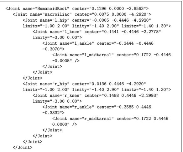
To make an introduction to the XML data format that we adopted for articulated figure modeling, a portion of the XML data for the human figure used is given in

Figure 3.1. The complete human figure in XML format is given in Appendix A.2. The Document Type Definition (DTD) of the human body representation that is used in XML format that defines humanoid is presented in Appendix A.1.

Figure 3.1: A portion of humanoid data in XML format.

The nodes in H-Anim 1.1 Specification (Humanoid, Joint and Segment) are used as elements in XML to construct a hierarchy that corresponds to the skele-ton. In this format, the following attributes are used for joint nodes. center attribute is used for positioning the associated element. name attribute specifies the name of associated element. limitx, limity, and limitz attributes are used for setting the upper and lower limits for the joint angles, respectively.

Although the data format stated above can be used for representing the full skeleton specified in the H-Anim standard, we do not need completely define all the joints in our application. The complete hierarchy is too complex for most of

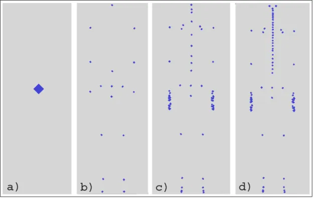
the applications. For example, in real-time applications such as games, there is no need to use the full set of joints. A simplified hierarchy will be more suitable for most of the games. Fortunately, in H-Anim 1.1 Specification document, four “Levels of Articulation” that contain the subsets of the joints are suggested. The body dimensions and level of articulations are suggested for information only and are not specified by the H-Anim standard. Behind the simplicity goal, one other reason for suggesting level of articulations is the compatibility. Conforming to a level of articulation, the animators could share their animations and humanoids to the same (or higher) level of articulation. After dissecting the level of articula-tion, a more simplified version of “Level of Articulation Two” seems appropriate for our work. Because, “Level of Articulation One” represents a typical low-end real-time 3D hierarchy and it does not contain information about the spine. Be-sides, the shoulder complex is not much detailed. On the other side, “Level of Articulation Two” represents much information that is needed about spine, skull and hands. “Level of Articulation Three” represents the full H-Anim hierarchy.

Figure 3.2: Level of articulations: a) level of zero, b) level of one, c) level of two, and d) level of three.

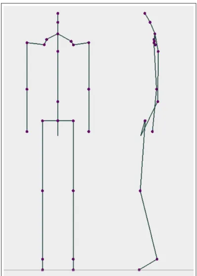
A front and left view of the skeleton corresponding to the XML based model in Appendix A.2 is represented in Figure 3.3.

Figure 3.3: Left and top view of the skeleton.

Moreover, a framework is implemented to parse the skeleton data and con-struct an abstract skeleton data type. C++ is used for the implementation of the system. All the classes are grouped in a package, named Hbody. The Hbody pack-age contains the following classes: Humanoid, Joint, Segment, Site, and Node.

The Hbody package supports the creation and manipulation of the body struc-ture defined by a file in XML format that conforms to the DTD given in Ap-pendix A.1. A simple XML parser, TinyXml [39], is used to parse the XML data.

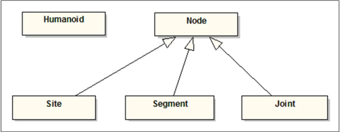
The UML class diagram is shown in Figure 3.4 to graphically illustrate the classes hierarchy for the system implementation.

Figure 3.4: UML class diagram of the Hbody package.

Humanoid class is used to define the abstract data type humanoid. It stores in-formation (such as author, copyright, gender of humanoid, etc) about humanoid. It can act as a group of hierarchical nodes. It also stores references to all Joints, Segments, and Site nodes in a vector structure for quick access to nodes. Briefly, Humanoid class serves as a wrapper for the humanoid.

Node class is the base class for the classes Joint, Segment and Site. This class stores a list of child nodes which is needed to define the hierarchy. Joint and Segment classes are used to define the joints and segments in human body structure. Site class is used as an end-effector for inverse kinematics. Joint, Segment and Site classes inherit the members and functionality of base class Node. So, all these classes can take part in the hierarchical structure constructed by using Node objects.

This package can be used to represent various articulated structures, like humans, animals and robots, since it is designed and implemented in a generic way.

Chapter 4

MOTION CONTROL

The control of human motion has always been a challenging problem in computer animation. Numerous studies in fields such as biomechanics, robotics, animation, ergonomics, and psychology are integrated to have realistic human motion control techniques. The motion control can be classified in two categories according to the level of abstraction that specifies the motion; low-level and high-level systems. A low-level system needs to specify the motion parameters (such as position, angles, forces, and torques) manually. In a high-level animation system, motion is specified by abstract terms such as “walk”, “run”, “grab that object”, “walk happily”, etc. At higher levels, the low level motion planning and control tasks are done by the machine. The animator just changes some parameters to obtain different kind of solutions. This study especially focuses on the low-level control of motion using kinematic methods. Spline-driven animation techniques are used to specify the characteristics of the motion. In addition, a high-level walking animation mechanism that make use of these low-level techniques are described.

4.1

Low-Level Control of Motion

In the study, spline-driven animation method is used as a low-level control mecha-nism. In this technique, motion characteristics of an object are specified by using splines. The trajectories of limbs (paths of pelvis, ankles in a human walking animation) in a human motion are controlled by splines. Besides, using a conven-tional keyframing technique the joint angles over time are determined by splines. Since splines are smooth curves, they can be used in interpolation of smooth mo-tions in space. Moving an object along a smooth path is supplied with smooth spline curves.

There are several different kinds of splines that are used for different kind of purposes in graphics applications. Cubic splines are one of them that have been extensively used. Since they require less calculations and memory and allow local control over the shape of the curve, cubic splines are the mostly preferred ones. We can use these splines not only in setting up paths for object motions but also in designing object shapes. One other advantage is that, compared with the lower-order polynomials it is more flexible for modeling arbitrary curve shapes [23].

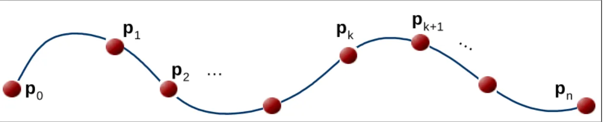
For a set of control points, cubic splines are generated by a piecewise poly-nomial curve that passes through every control points. We can denote the curve with:

pk= (xk, yk, zk), k = 0, 1, 2, ..., n (4.1)

The cubic spline generated from these control points is presented in Figure 4.1. The parametric cubic polynomial that is to be fitted between each pair of control points is represented by followings:

p_k pk+1 p_n p₀ p₁ p₂ … …

Figure 4.1: A piecewise continuous cubic-spline interpolation of n + 1 control points.      xu yu zu     =      axu3+ bxu2 + cxu + dx ayu3+ byu2 + cyu + dy azu3+ bzu2+ czu + dy     , (0 ≤ u ≤ 1) (4.2)

One class of cubic splines, natural cubic splines, is one of the first spline curves to be developed for needs of computer animation. This curve is a mathematical representation of the original drafting spline. It has C2 _{continuity because, the}

formulation of these splines requires two adjacent curve section to have the same first and second parametric derivatives. Beyond the advantage of being a mathe-matical model for drafting spline, natural cubic splines have a big drawback that they do not allow local control. That means changing the position of any control point results with a alteration in the entire curve.

Hermite spline is another class of cubic splines that is represented by an interpolating cubic polynomial with a specified tangent at each control point [5]. Contrary with the natural cubic splines, Hermite splines provide local control because each curve section is only related with its endpoints. A sample Hermite curve section is illustrated in Figure 4.2.

Although Hermite polynomials can be useful for some digitizing applications, for most computer graphic applications, it is preferable to generate spline curves without requiring input values for curve slopes or other geometric constraints. Detailed information about Hermite splines can be found in [23].

Figure 4.2: Parametric point function P (u) for a Hermite-spline section.

Like Hermite splines, Cardinal splines interpolates piecewise cubics with spec-ified endpoint tangents at the boundary of each curve section with an exception that Cardinal splines does not require the values for the endpoint tangents. In-stead, the value of the slope of a control point is calculated from the coordinates of the two adjacent points.

Figure 4.3: Parametric point function P (u) for a Cardinal-spline section.

A Cardinal spline section is specified with four consecutive control points. The middle two points are the endpoints and the other two are used to calculate the slope of the endpoints. As it is seen in the Figure 4.3, if we present the parametric cubic point function for the curve section between control points Pk

and Pk+1with P (u) then, the boundary conditions for the Cardinal spline section

P (0) = pk, P (1) = pk+1, P0_{(0) =} 1 2(1 − t)(pk+1− pk−1), P0_{(1) =} 1 2(1 − t)(pk+2− pk), (4.3)

where parameter t, tension parameter, controls how loosely or tightly the Car-dinal spline fits the control points. When t=0, this class of curves are named as Catmull-Rom splines, or Overhauser splines [13].

We can generate the boundary conditions formulation as:

Pu = h u3 u2 u 1 i · MC·          pk−1 pk pk+1 pk+2          , (4.4)

where the Cardinal matrix is:

MC =          −s 2 − s s − 2 s 2s s − 3 3 − 2s −s −s 0 s 0 0 1 0 0          , s = (1 − t) 2 , (4.5)

where t is the tension parameter.

One other cubic spline class is the Kochanek-Bartels splines, which is an extension of the Cardinal splines. Kochanek-Bartels splines include two addi-tional parameters in order to have the flexibility in adjusting the shape of the curve sections. Kochanek-Bartel splines are especially designed for modeling the animation paths.

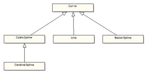
In our system we used Cardinal splines, which are very powerful and have controllable input control points fitting mechanism with a tension parameter. The UML class diagram of the implemented curve classes is shown in Figure 4.4 that graphically illustrates the classes.

Figure 4.4: UML class diagram of the Curve package.

The paths for pelvis, ankle and wrist motions are specified using Cardinal spline curves. These are considered as position curves. Besides, a velocity curve is specified independently for each object. Thus, just affecting the velocity curve, characteristics of the motion can be changed. Steketee and Badler were the first to recognizing this powerful method [37]. They called this velocity curve as “kinetic spline”. The method is called “double interpolant” method. Kinetic spline may also be interpreted as a distance curve. Given a distance curve or velocity curve, velocity curve or distance curve can be easily calculated.

Our application makes use of the “double interpolant” by enabling the user to specify a position spline and a kinetic spline. The kinetic spline, Velocity curve, V(t), is commonly used as the motion curve. However, V(t) can be integrated to determine distance curve, S(t). These curves are represented in two-dimensional space for easy manipulation. Position curve is a three-dimensional curve in space,

through which the object moves. Control of motion involves editing the position and kinetic splines. In our application velocity curves, and distance curves are straight lines and Cardinal splines, respectively. Line, which graphically depicts a straight line, and CardinalSpline classes in Figure 4.4 are used to represent the curves.

Furthermore, a problem arises while moving an object along a given position spline because of the parametric nature of cubic splines. Suppose we had a velocity curve and a position curve to control the motion. We can find the distance travelled at a given time by having the integral of the velocity curve with respect to time. Now we must find a point along the position spline, where the computed distance is mapped.

If we formulate the problem; we have a path specified by a spline Q(u), (0 ≤ u ≤ 1) and we are looking for a set of points along the spline such that, the distance travelled along the curve between consecutive frames is constant. Basically, these points can be computed by evaluating Q(u) at equal values of

u. But this requires the parameter u to be proportional to the arclength, the

distance travelled along the curve. Unfortunately, this is not the case in general. In the special cases where the parameter is proportional to arclength, the spline is said to be parameterized by arclength. Figure 4.5 illustrates a spline with 10 points of equal intervals of u and 10 points located at equal intervals of arclength. As it is seen from the figure, without the arclength parameter an object can hardly move with a uniform speed along a spline. This arclength problem can be solved by using the arclength parameterization of spline curve [21, 41].

Cardinal spline curves provide the required functionality for motion control. They can be constructed with a few set of control points and can be manipulated easily. Having these advantages, a motion control system is implemented in which the animator constructs the position and kinetic splines for the joints ankle, wrist and pelvis. Figures 4.8 and 4.9 illustrate the distance and velocity

Figure 4.5: Intervals of equal parametric length (outlined arrowheads) do not correspond to equal intervals of arclength (black arrowheads) (reprinted from [41]).

curves that utilizes the CardinalSpline and Line classes. In Figures 6.2 and 6.3, the position curve that utilizes the CardinalSpline class is shown. The animator interactively shapes the curves, and view the resulting animation in real time. Double interpolant method enables the animator to change characteristics of the motion independently. This can be done by editing different curves that correspond to the position in 3D space, distance, and velocity curves independent from each other. However, the result of change in kinetic spline curve should be controlled in the position curve in order to have the desired motion.

After constructing the position curves for end effectors like wrist and ankles, goal-directed motion control technique is used to determine the joint angles of shoulder, hip, elbow and knee over time. Using a inverse kinematics method to determine the position and orientation of upper joints along the hierarchy really simplifies the control of motion. The animator only moves the end-effector and the orientations of other links in the hierarchy are computed by inverse kinematics.

In addition, our system enables the user to define the joint angles which are not computed by the inverse kinematics program. Using a conventional keyframing technique, the joint angles over time can be specified by the user. Cardinal splines are used to have a smooth interpolation of joint angles.

In this fashion, the system provides a low-level animation system to the user in which one can obtain any kind of motion by specifying a set of spline curves for position, distance and joint angles over time. Besides, our application enable the user to save and load, and animate the defined motions. The user interface of the application is described in Appendix C.

Furthermore, using these low-level techniques, a high-level motion mechanism for walking is provided which is explained in the following section.

4.2

Human Walking Behaviour

Most of work in motion control has aimed to provide high level controls to pro-duce complex motions like walking. Kinematics and dynamic approaches for hu-man locomation are described by hu-many researchers [4, 8, 10, 11, 19, 25, 44, 48]. Many approaches are introduced for the animation of human walking. A survey of human walking is given in [32].

In our system walking motion can be controlled using kinematic approaches in high level by allowing the user to specify a few number of locomotion parameters. Specifying the straight travelling path on flat ground without obstacles and the speed of locomotion, our system generates the walking automatically, by com-puting the 3D path information and the low-level kinematics parameters of body elements. Furthermore, some extra parameters such as the size of walking step, the time elapsed during double-support, rotation, tilt, and lateral displacement of pelvis can be adjusted by the user to have a different walking motion.

Walking is a smooth, symmetric motion in which the body, feet, and hands move rhythmically in the required direction with a speed. Basically, it can be characterized as the succession of phases separated by the state of foots because, the feet drive the main part of the animation. During walking, foot has contact

with the ground (footstrikes) and leaves the ground (takeoffs) successively. The

stride is defined as the walking cycle in which four footsrikes and takeoff events

occur. The part of this cycle, which is between the takeoffs of the two feet, is called a step. In this concept, the phases for each leg can be classified into two phases: The stance and the swing phases. The stance phase is the period of support. The swing phase is the non-support phase. In the locomotion cycle, each leg pass through both the stance and swing phases. In the cycle, there is also a period of time where both of the legs are in contact with the ground. The phase is called as double-support. The phases of walking cycle can be seen in Figure 4.6 double support Single support (left) right swing left swing left stance right stance 50% 0% 100% Single support (right) double support states phases lFS rTO rFS lTO lFS

Figure 4.6: Locomotion cycle for bipedal walking (adopted from [32]).

Furthermore, walking has some special characteristics. One foot is in contact with the ground at all times and for a period both of the feet are in contact with the ground. In addition the motion is cyclic. These characteristics of walking really simplify the control mechanism. However, natural human walking animation is a challenging problem. The kinematics nature of walking should be more dissected for a realistic walking motion. For this purpose, Saunders et al. defined a set of gait determinants, which mainly describe the movement of pelvis motion [33]. These determinants are compass gait, pelvic rotation,

pelvic tilt, stance leg flexion, planar flexion of the stance angle, and lateral pelvic displacement.

Figure 4.7: Walking gaits: (a) compass gait, (b) pelvic tilt, (c) plantar flexion, (d) pelvic rotation, (e) stance leg inflexion, and (f) lateral pelvic displacement (reprinted from [41]).

1. Compass gait (Figure 4.7(a)) The legs remain straight, moving in parallel planes. The pelvis moves in a series of arcs whose radius is determined by the leg length.

2. Pelvic tilt (Figure 4.7(b)) If the pelvis is allowed to tilt as well as rotate the arc of its trajectory can be further flattened. In practice the hip on the ‘swing’ side of the walk falls below the hip on the ‘stance’ side. This lowering occurs immediately after the end of the double support phase and the ‘toe-off’ of the swing leg. Introducing a pelvic tilt necessarily involves a knee flexion of the swing leg.

3. Plantar flexion of the stance angle (Figure 4.7(c)) The transition between the double support phase and the swing phase is made smoother if the angle of the stance leg moves down just prior to toe-off. This means that the foot must flex with respect to the shin.

4. Pelvic rotation (Figure 4.7(d)) Allowing the pelvis to rotate about a vertical axis through its center enables the length of the step to be increased and the arc to be flattened. Saunders et al. quote ±3 degrees for the amplitude of this motion.

5. Stance leg flexion (Figure 4.7(e)) The next elaboration is stance leg flexion where the pelvic trajectory arc is further flattened.

6. Lateral pelvic displacement (Figure 4.7(f)) Normal walking involves dis-placement of the pelvis from side to side, as the weight is transferred from one limb to another [41].

In our system, compass gait, pelvic rotation, pelvic tilt, and lateral pelvic displacement is considered. In pelvic rotation, pelvis rotates about the body to the left and the right, relative to the walking direction. Saunders et al. quote 3 degrees for the amplitude in a normal walking gait. In normal walking, the hip of the swing leg falls slightly below the hip of the stance leg. This event occurs

for the side of swing leg, after the end of the double support phase. 5 degrees is considered for the amplitude of pelvis tilt. In lateral pelvic displacement, the pelvis moves from side to side. Immediately after the double support, the weight is transferred from center to the stance leg. So, a pelvis moves alternately during a normal walking. Moreover, individual gait variations can be obtained by determining the parameters of these pelvis activities. Our system enables the user to specify these parameters and observe the walking animation carefully.

The main parameters of walking behavior are the velocity and step length. Walking can have different variations by changing these parameters. However, experimental results show that these parameters are somehow related. Inman et al. [33] related the walking speed to walking cycle time and Bruderlin and Calvert [10] stated the correct time durations for a locomotion cycle. Based on the experimental works on walking, the followings can be stated:

velocity = stepLength × stepF requency (4.6)

stepLength = 0.004 × stepF requency × bodyHeight (4.7) Experimental data shows that maximum value of stepF requency is 182 steps per minute. Time for a cycle can be calculated from the step frequency:

tcycle = 2 × tstep = 2

stepF requency (4.8)

Using the Figure 4.6, time for double support (tds) and and the single support phases can be calculated using the formula :

tstep = tstance − tds (4.9)

tstep = tswing + tds (4.10) Based on the experimental results tds is calculated as [33]:

tds = (−0.0016 × stepF requency + 0.2908) × tcycle (4.11) Although tds could be calculated automatically if the stepF requency is given, it is sometimes convenient to redefine tds to have walking animations with various characteristics.

By utilizing the groups of formula, which define the kinematics of walking, a velocity curve (time vs. velocity) is constructed for the left and right ankles. Figure 4.8 is shown to graphically illustrate the velocity of left and right ankles versus time. The distance curves shown in Figure 4.9 are automatically generated using the velocity curves. Ease-in, ease-out effect which is generated by speed up and slow down of the ankles can be seen on distance curves.

Figure 4.8: The velocity curve of a) left ankle and b) right ankle.

Figure 4.9: The distance curve of a) left ankle and b) right ankle.

In conclusion, a high-level walking motion is obtained in our system by using the parameters like walking speed, time elapsed during double support phase, and gait determinant parameters like pelvis rotation, pelvis tilt, and lateral dis-placement. Figures in Chapter 6.1 illustrate the obtained walking motion.

Chapter 5

IKAN

5.1

Motion of the Skeleton

Our system uses the kinematics based methods for motion control. Forward and inverse kinematics are two main approaches in kinematic animation. Our work focuses on the analytical inverse kinematics methods in which, the goal orientations are specified and the position or rotation of joints are computed by using analytical methods. Moving a hand to grab an object or placing the foot to a desired position requires the usage of inverse kinematics methods.

In our study, we used an inverse kinematics package, called IKAN. IKAN is a complete set of inverse kinematics algorithms for an anthropomorphic arm or leg. It uses a combination of analytic and numerical methods to solve gen-eralized inverse kinematics problems including position, orientation, and aiming constraints. IKAN methodology is explained in [15].

IKAN provided us the required functionality to control the arm and leg of human model. For the arm, with the goal of putting the wrist in the desired

location, IKAN computed the joint angles for the shoulder and elbow. In the case of leg, rotation angles for hip and knee is calculated.

IKAN’s methodology is constructed on a 7 DOF fully revolute open kinematic chain with two spherical joints connected by a single revolute joint. Although the primary work is on the arm, the methods are suitable for a leg because, the kinematic chain of leg is similar to the kinematic chain of the arm. In the arm model, the spherical joints with 3 DOFs are shoulder and wrist; the revolute joint with 1 DOF is elbow. In the leg model, the spherical joints with 3 DOFs are hip and ankle; the revolute joint with 1 DOF is knee.

The details of how we incorporated IKAN with our work is as follows. Ex-plaining the details for an arm will unravel the solution for the leg. Because, leg and arm are both considered being similar human arm-like (HAL) chains, only some parameters change in the case of leg.

First of all, the right-handed coordinate system illustrated in Figure 5.1 is assumed at all the joints (shoulder, elbow, and wrist in the case of the arm).

The elbow is considered as to be parallel to the length of the body at rest condition. The z-axis is from elbow to wrist. The y-axis is perpendicular to z-axis and it is the axis of rotation for elbow. The x-axis is pointing away from the body along the frontal plane of the body. The x, y, and z axes form a right-handed coordinate system.

Similar coordinate systems are assumed at the shoulder and at the wrist. The projection axis is always along the limb and the positive axis points away from the body perpendicular to the frontal plane of the body. The projection axis differs for left and right arm. Wrist to elbow and elbow to shoulder transformations are calculated since they are needed to initialize the SRS object in IKAN. The initialization process is as follows:

Figure 5.1: Example arm showing the selection of projection and positive axis (reprinted from [15]).

SRS ikSolver(T, S, a, p);

where T is the elbow to shoulder transformation matrix, S is the wrist to elbow transformation matrix, a is the projection axis, and p is the positive axis for the arm. z-axis and x-axis are used as parameters for projection axis and positive axis, respectively for the left HAL chains of left arm and left leg. Negative z-axis and x-axis are used as parameters for projection axis and positive axis, respectively for the right HAL chains of right arm and right leg.

5.2

Implementation Details

We reused the functionality provided in the C++ classes of JackPlugin, which is distributed in the IKAN package as an example source for the usage of basic IK classes. Actually, the classes of JackPlugin do not have a good object ori-ented structure. In that package the class Limb has the main functionality. We reused almost the whole functionality of the class Limb in our class HALChain. We stated a better oriented structure to take the advantage of object-oriented paradigm. C++ class structure, data encapsulation, inheritance, and polymorphism mechanism provided us much more cleaner and easier-to maintain code, and it allowed easier extensions. The class diagram in Figure 5.2 depicts the structure.

Figure 5.2: UML class diagram for IKAN classes that is used in our system.

The attributes and operations of the classes are given in Appendix B. The terms R1-joint, R-joint, R2-joint are used extensively. They are the joints in a HAL chain. In the case of the arm, R1-joint refers to shoulder where R-joint refers to the elbow and R2-joint refers to the ankle.

The arm is initialized with a Humanoid object and the name of the shoulder, elbow and wrist joints. In this initialization part, the transformation matrices (T and S) are computed and the inverse kinematics solver (SRS object) is initialized.

The methods setGoalPos, solverJoint are the main operations of the HALChain class. Call to the wrapper method setGoalPos is delegated to the functional class SRS. setGoalPos function sets the goal position for the end-effector. If the goal is feasible, the swievel angle of R-joint (elbow or knee) is calculated and the rotation matrix for the R-joint is computed using the swievel angle. Besides, if the upper and lower joint angle limits are specified, the valid angle ranges in which the R-joint can swievel is calculated. In solveRJoint method, the largest valid range is selected and the swievel angle, which is the middle value of this range, is used. Using this swievel angle value, the rotation matrix of R1-joint is computed by utilizing the SRS object’s solveR1 method. By the way, the position of the R-joint can be calculated by SRS’s AngleToPos method, but it is not needed in our application, after the rotation matrices of R1 and R-joints appeared. Through this brief explanation it can be inferred that, the goal position is calculated relative to the R1-joint, because the R1-joint does not need to be static. Besides, after the rotation matrices are found, they need to be transformed into the global coordinate system. For example, in a inverse kinematics application such as walking animation, the pelvis and the ankle is always moving. There exists many goal positions. In each intermediate step, the goal position is first calculated relative to the pelvis. The orientation matrices of the pelvis and knee are calculated in local coordinate system. Then, they are transformed into the global coordinates.

The end-effectors positions and the orientations of joints can be seen in Fig-ure 5.3. From the knowledge of end-effectors, the joint angles are found auto-matically.