NANOMECHANICAL
CHARACTERIZATION OF MATERIALS BY
ENHANCED HIGHER HARMONICS OF A
TAPPING CANTILEVER
a dissertation submitted to
the department of electrical and electronics
engineering
and the institute of engineering and science
of bilkent university
in partial fulfillment of the requirements
for the degree of
doctor of philosophy
By
M¨ujdat Balantekin
May, 2005
I certify that I have read this thesis and that in my opinion it is fully adequate, in scope and in quality, as a dissertation for the degree of doctor of philosophy.
Prof. Dr. Abdullah Atalar (Supervisor)
I certify that I have read this thesis and that in my opinion it is fully adequate, in scope and in quality, as a dissertation for the degree of doctor of philosophy.
Prof. Dr. Hayrettin K¨oymen
I certify that I have read this thesis and that in my opinion it is fully adequate, in scope and in quality, as a dissertation for the degree of doctor of philosophy.
I certify that I have read this thesis and that in my opinion it is fully adequate, in scope and in quality, as a dissertation for the degree of doctor of philosophy.
Prof. Dr. Yusuf Ziya ˙Ider
I certify that I have read this thesis and that in my opinion it is fully adequate, in scope and in quality, as a dissertation for the degree of doctor of philosophy.
Prof. Dr. Tayfun Akın
Approved for the Institute of Engineering and Science:
Prof. Dr. Mehmet B. Baray Director of the Institute
ABSTRACT
NANOMECHANICAL CHARACTERIZATION OF
MATERIALS BY ENHANCED HIGHER HARMONICS
OF A TAPPING CANTILEVER
M¨ujdat Balantekin
Ph.D. in Electrical and Electronics Engineering Supervisor: Prof. Dr. Abdullah Atalar
May, 2005
In a tapping-mode atomic force microscope, the periodic interaction of the tip with the sample surface creates a tip-sample interaction force, and the pure si-nusoidal motion of the cantilever is disturbed. Hence, the frequency spectrum of the oscillating cantilever contains higher harmonics at integer multiples of the excitation frequency. In this thesis, we utilize one of the higher harmonics of a vibrating cantilever to investigate the material properties at the nanoscale. We show analytically that the amplitudes of the higher harmonics increase monoton-ically for a range of sample stiffness, if the interaction is dominated by elastic force. We propose a method in which the cantilever is excited at a submultiple of its resonant frequency (w1/n) to enhance the nth harmonic. The numerical
simulations are performed to obtain the response of the tip-sample system for the proposed method. The proposed method is modified to eliminate the chaotic system response observed in the very high harmonic distortion case. The exper-iments are carried out to see if the enhanced higher harmonic can discriminate the material variations in heterogeneous samples and to find how it is related to the topography changes on the homogeneous sample surfaces. We show that the enhanced higher harmonic can be utilized to map material heterogeneity in polymer blends with a very high signal-to-noise ratio. The surface features ca. 100 nm in size are clearly resolved. A comparison is also made to conventional tapping-mode topography and phase imaging.
Keywords: Atomic force microscope, tapping-mode, vibrating cantilever, en-hanced higher harmonics, nanomechanical material properties.
¨
OZET
T˙ITRES¸EN KALDIRACIN GEL˙IS¸T˙IR˙ILM˙IS¸ Y ¨
UKSEK
HARMON˙IKLER˙I VASITASIYLA MADDELER˙IN
NANOMEKAN˙IKSEL N˙ITELEND˙IR˙ILMES˙I
M¨ujdat Balantekin Elektrik M¨uhendisli˘gi, Doktora Tez Y¨oneticisi: Prof. Dr. Abdullah Atalar
Mayıs, 2005
Atomik kuvvet mikroskobunun vurma-modu’nda, kaldıra¸c ucunun denek y¨uzeyiyle periyodik etkile¸simi u¸c-denek etkile¸sim kuvvetini do˘gurur ve kaldıracın saf sin¨usoidal devinimi bozulur. Bu nedenle, titre¸sen kaldıracın tayfı uyarma frekansının tam katlarında y¨uksek harmonikler ihtiva eder. Bu tezde, nano ¨ol¸cekteki materyal ¨ozelliklerini ara¸stırmak i¸cin titre¸sen kaldıracın y¨uksek har-moniklerinin bir tanesininden faydalanıyoruz. E˘ger etkile¸sime elastik kuvvet ege-mense, y¨uksek harmoniklerin genli˘ginin belirli bir denek sertli˘gi aralı˘gında mono-ton bir ¸sekilde arttı˘gını analitik olarak g¨osterdik. n’inci harmoni˘gi geli¸stirmek i¸cin, kaldıracın kendi rezonans frekansının tam b¨oleninde (w1/n) uyarıldı˘gı
bir y¨ontem ¨onerdik. U¸c-denek sisteminin ¨onerilen y¨onteme tepkisini elde et-mek i¸cin sayısal benzetimler icra edildi. C¸ ok y¨uksek harmonik bozunumu durumunda g¨ozlenen d¨uzensiz sistem tepkisini bertaraf etmek i¸cin ¨onerilen y¨ontem biraz de˘gi¸stirildi. Geli¸stirilmi¸s y¨uksek harmoni˘gin ¸cokt¨urel denek-lerdeki madde de˘gi¸simlerini ayırt edebilirli˘gini g¨ormek ve tekt¨urel deneklerin y¨uzeyindeki topografya de˘gi¸simlerine nasıl ba˘glı oldu˘gunu bulmak amacıyla deneyler yapıldı. Geli¸stirilmi¸s y¨uksek harmoni˘gin polimer karı¸sımlarındaki materyal ¸cokt¨urelli˘ginin ¸cok y¨uksek bir sinyal/g¨ur¨ult¨u oranı ile resimlenmesi i¸cin kullanılabilece˘gini g¨osterdik. Takriben 100 nm boyutundaki y¨uzey yapıları net bir ¸sekilde g¨or¨unt¨ulendi. Ayrıca geleneksel vurma-modu’nun topografya ve faz g¨or¨unt¨ulemesine kar¸sıla¸stırma yapıldı.
Anahtar s¨ozc¨ukler : Atomik kuvvet mikroskobu, vurma modu, titre¸sen kaldıra¸c, geli¸stirilmi¸s y¨uksek harmonikler, nanomekanik madde ¨ozellikleri.
Acknowledgement
There are many people who contributed to this research work. But, first of all, I would like to express my sincere gratitude to Prof. Abdullah Atalar who gave me a chance to work with him during the past few years. Without his invaluable guidance and endless support, I could not finish this study.
I would like to thank the members of the thesis committee, Prof. Hayrettin K¨oymen, Prof. Ekmel ¨Ozbay, Prof. Yusuf Ziya ˙Ider, and Prof. Tayfun Akın for reading and commenting on the thesis.
I would like to thank Dr. Ahmet Oral who provided the part of the experi-mental setup and helped me a lot in his laboratory.
Many thanks to ¨Ozg¨ur S¸ahin for sending the tipholder.
It is a pleasure to thank Prof. Salim C¸ ıracı for providing a conference support. Special thanks to Erg¨un Hırlako˘glu for providing the laboratory equipment. Special thanks to Dr. Soner Kılı¸c for the polymer samples. I would like to thank Dr. Ahmet Oral one more time for the suggestion of analyzing a block copolymer sample.
It is an obligation for me to thank Dr. Necmi Bıyıklı for the excellent prepa-ration of many samples. I also thank Bayram B¨ut¨un for the test samples.
Special thanks to Murat G¨ure for SEM micrographs.
I would like to thank all the friends, Muharrem, Koray, M¨unir, Fatih, and G¨oksel, in the physics department.
I would also like to thank Dr. Levent De˘gertekin and his students G¨u¸cl¨u Onaran and Zehra Parlak who conducted some experiments for us.
Contents
1 Introduction 1
1.1 Atomic Force Microscopy . . . 1
1.1.1 Contact Mode . . . 3
1.1.2 Hopping Mode . . . 3
1.1.3 Tapping Mode . . . 3
1.1.4 Non-contact Mode . . . 4
1.2 Organization of the Thesis . . . 4
2 Nanomechanical Surface Characterization Techniques 6 2.1 Nanoindentation . . . 6
2.2 Force Modulation Microscopy . . . 7
2.3 Atomic Force Acoustic Microscopy . . . 7
2.4 Pulsed Force Mode . . . 8
2.5 Dynamic Force Spectroscopy . . . 8
2.7 Higher Harmonic Imaging . . . 9
3 Analytical Evaluation of Higher Harmonics 10 3.1 Interaction Modeling . . . 11
3.2 Tip-sample Interaction Forces . . . 13
3.2.1 Conservative Forces . . . 13
3.2.2 Dissipative Forces . . . 17
3.3 Amplitude Damping, Maximum Force and Contact Time . . . 18
3.4 Results and Discussion . . . 23
4 Numerical Analysis for Enhanced Higher Harmonics 27 4.1 Higher Harmonic Enhancement . . . 28
4.2 Simulation Details . . . 30
4.3 Simulation Results . . . 31
4.4 Comparison to Analytical Solution . . . 40
5 Experimental Setup 50 5.1 Instruments . . . 50 5.2 Measurement Cantilever . . . 52 5.3 Noise . . . 52 5.4 Experimental Problems . . . 56 6 Experimental Results 59
6.1 Test Samples . . . 60
6.1.1 A Square-patterned GaAs Substrate . . . 60
6.1.2 A Square-patterned Photoresist on GaAs Substrate . . . . 68
6.2 Heterogeneous Polymers . . . 78
6.2.1 20:80 Polystyrene/Polyisoprene Blend . . . 82
6.2.2 80:20 Polystyrene/Polyisoprene Blend . . . 91
6.2.3 50:50 Polystyrene/Polyisoprene Blend . . . 99
6.2.4 Polystyrene-block -Polyisoprene-block -Polystyrene Copolymer106 6.3 A Scratched Square-patterned GaAs Substrate . . . 117
6.4 Summary and Discussion . . . 128
7 Conclusions 133
A Experimental Setup 150
B Cantilever Specifications 154
List of Figures
3.1 (a) Flexural-beam model. (b) Point-mass model. . . 12 3.2 van der Waals forces. The tip oscillates above the sample surface. 14 3.3 Elastic contact force. The tip touches the sample in a fraction of
its oscillation period. . . 16 3.4 Normalized maximum repulsive force Fmax/(βAα
1E) (thin lines)
and Fmax/f (thick lines) are plotted as a function of normalized mean tip-surface distance γ for varying values of E∗ and f
1 for a
cylindrical tip. . . 21 3.5 Normalized maximum repulsive force Fmax/(βAα1E) (thin lines)
and Fmax/f (thick lines) are plotted as a function of normalized mean tip-surface distance γ for varying values of E∗ and f
1 for a
conical tip. . . 22 3.6 A variation of the first four normalized harmonic amplitudes |Λ(γ)|
as a function of normalized effective tip-sample elasticity λ−1(γ) for a cylindrical tip. It is assumed that An ¿ A1. The vertical
dashed line marks the γ = 0 location. . . . 24 3.7 A variation of the first four normalized harmonic amplitudes |Λ(γ)|
as a function of normalized effective tip-sample elasticity λ−1(γ) for a conical tip. It is assumed that An ¿ A1. Vertical dashed and
4.1 Higher harmonic enhancement by matching to a flexural resonance. 29 4.2 Electrical equivalent of mechanical point-mass model. . . 31 4.3 Simulation results for the second and third harmonics when the
cantilever is driven at w = w1/2 and w = w1/3, respectively.
A2/A0 (stars) and A3/A0 (asterisks) are plotted for a paraboloidal
tip with a radius of curvature R = 10 nm. The simulation param-eters are A0 = 100 nm, A1/A0 = 0.99, Q = 100, and k = 1 N/m.
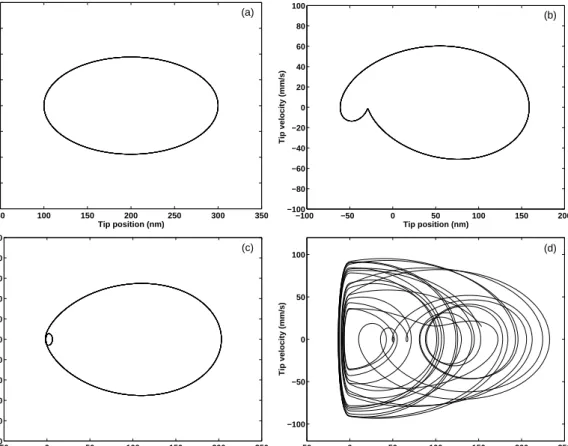
A vertical dashed line separates the region I (γ < 0) and region II (γ > 0), whereas the dotted line indicates the beginning of chaotic region for the third harmonic. Those locations for the second har-monic are very close to these lines and not shown for clarity. . . . 32 4.4 Phase diagrams for four different elastic samples with w = w12and
w1 = 2π×120 krad/s. (a) Free, (b) E∗ = 1 MPa, (c) E∗ = 1 GPa,
and (d) E∗ = 6 GPa. Ten oscillation cycles are plotted in each graph. . . 34 4.5 Tip motions taken from simulations for three different elastic
sam-ples when the cantilever is excited at w = w1/2. The position of
the undeformed sample surface is indicated by the horizontal line. 35 4.6 Left-hand axis: Simulation results for A2 (w = 0.98w1/2) marked
by stars and A3 (w = 0.97w1/3) marked by asterisks in the
per-centage of A0 with the same parameters of Figure 4.3. The vertical
dashed line indicates the γ = 0 location. Right-hand axis: Simu-lation results for the conventional case (w = w1). A2 is marked by
circles and A3 is marked by rectangles in the percentage of A0 at
A1/A0 = 0.6. The other parameters are the same. . . . 37
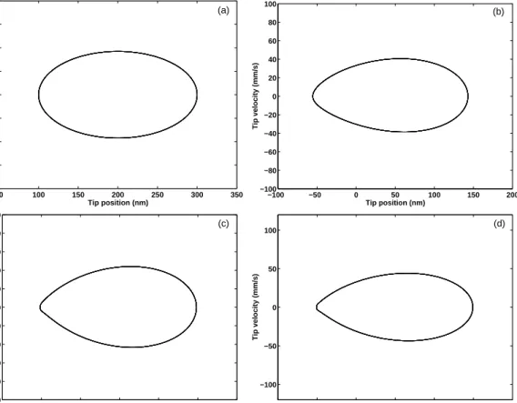
4.7 Phase diagrams for the same cases of Fig. 4.4 at w = 0.98w12. (a)
Free, (b) E∗ = 1 MPa, (c) E∗ = 1 GPa, and (d) E∗ = 6 GPa. Ten oscillation cycles are plotted in each graph. . . 38
4.8 (a) Fundamental component of interaction force as a function of normalized frequency w/w1for two different set points. (b) A close
looking around the resonance frequency for A1/A0 = 0.99. . . . . 39
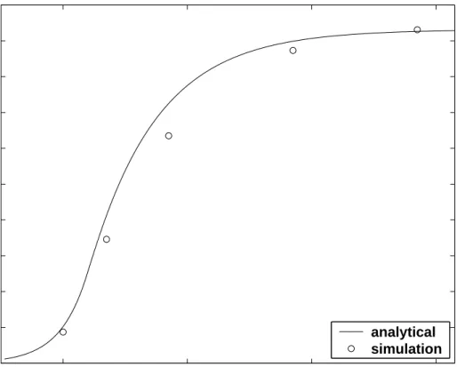
4.9 The variation of the second harmonic amplitude A2as a function of
effective tip-sample elasticity E∗ at w = 0.95w
1/2 and A1/A0 = 0.99. 40
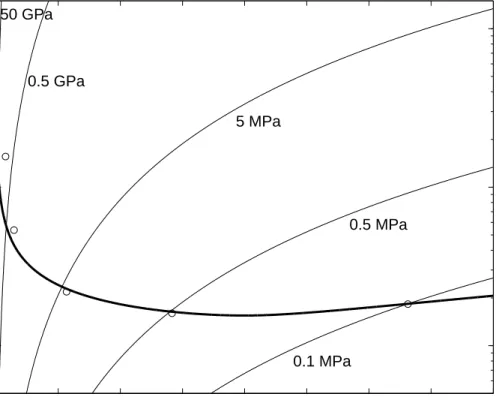
4.10 Tip position and 10×Force in one oscillation cycle. Simulation results are shown by thick dashed lines and analytical solutions are shown by thin solid lines at w = 0.95w1/2 and A1/A0 = 0.99.
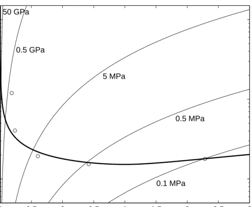
(a) E∗ = 50 GPa, (b) E∗ = 0.5 GPa, (c) E∗ = 5 MPa, (d) E∗ = 0.5 MPa, and (e) E∗ = 0.1 MPa. . . . 42 4.11 Maximum applied force versus normalized mean tip-surface
dis-tance. Analytical solutions (the intersection points of solid lines) and the simulation results (circles) at w = 0.95w1/2 and A1/A0 =
0.99 for different samples. . . . 43 4.12 The variation of the second harmonic amplitude A2as a function of
effective tip-sample elasticity E∗ at w = 0.98w
1/2 and A1/A0 = 0.99. 44
4.13 Tip position and 10×Force in one oscillation cycle. Simulation results are shown by thick dashed lines and analytical solutions are shown by thin solid lines at w = 0.98w1/2 and A1/A0 = 0.99.
(a) E∗ = 50 GPa, (b) E∗ = 0.5 GPa, (c) E∗ = 5 MPa, (d) E∗ = 0.5 MPa, and (e) E∗ = 0.1 MPa. . . . 45 4.14 Maximum applied force versus normalized mean tip-surface
dis-tance. Analytical solutions (the intersection points of solid lines) and the simulation results (circles) at w = 0.98w1/2 and A1/A0 =
0.99 for different samples. . . . 46 4.15 The variation of the second harmonic amplitude A2 as a function
of effective tip-sample elasticity E∗ at w = w
4.16 Tip position and 10×Force in one oscillation cycle. Simulation results are shown by thick dashed lines and analytical solutions are shown by thin solid lines at w = w1 and A1/A0 = 0.8. (a)
E∗ = 50 GPa, (b) E∗ = 0.5 GPa, (c) E∗ = 5 MPa, (d) E∗ = 0.5 MPa, and (e) E∗ = 0.1 MPa. . . . 48 4.17 Maximum applied force versus normalized mean tip-surface
dis-tance. Analytical solutions (the intersection points of solid lines) and the simulation results (circles) at w = w1 and A1/A0 = 0.8 for
different samples. . . 49 5.1 Schematic experimental setup. . . 51 5.2 SEM micrograph of the cantilever showing both the sensor and
actuator parts. (a) Top view. (b) Side view. . . 53 5.3 SEM micrograph of the sensor. (a) Top view. (b) Side view. . . . 54 5.4 SEM micrograph of the tip in (a) and the tip end in (b). . . 55 5.5 Amplitude and phase variations of the coupled voltage. . . 58 6.1 Optical micrographs of a square-patterned GaAs substrate at ×50
magnification in (a) and ×100 magnification in (b) and (c). . . . 61 6.2 Enhanced third harmonic imaging of a square-patterned GaAs
sub-strate. (a) Error, (b) Topography, (c) Third harmonic amplitude, (d) Topography (median filtered), and (e) Third harmonic am-plitude (image contrast is reversed). The variation from black to white is 2.7 nm in (a), 340 nm in (b), 0.54 nm in (c), and 290 nm in (d). Image parameters: Scan size = 10×10 µm, Pixel size = 256×256, Scan speed = 0.8 µm/s. Operating parameters: A0 ≈ 1.6 nm, A1/A0 = 1.2, w = 0.97w13. . . 62
6.3 Three-dimensional views of the sample in Fig. 6.2. (a) Error, (b) Topography, and (c) Third harmonic amplitude (inverted colors). 63 6.4 Third harmonic amplitude (green), surface topography (blue), and
error amplitude (divided by -10 to fit) (black) variations across the line indicated in Fig. 6.2 (b). . . 64 6.5 Histograms of (a) Error, (b) Surface height, and (c) Third
har-monic. . . 65 6.6 Conventional tapping-mode imaging of a square-patterned GaAs
substrate. (a) Error, (b) Topography, (c) Phase, (d) Topography (median filtered), and (e) Phase (image contrast is reversed). The variation from black to white is 9.4 nm in (a), 300 nm in (b), 30o in (c), and 270 nm in (d). Image parameters: Scan size = 10×10 µm, Pixel size = 256×256, Scan speed = 0.8 µm/s. Operating param-eters: A0 ≈ 12.9 nm, A1/A0 = 0.78, w = w1. . . 66
6.7 Three-dimensional views of the sample in Fig. 6.6. (a) Error, (b) Topography, and (c) Phase (inverted colors). . . 67 6.8 Surface topography (blue), error amplitude (multiplied by 10 to
fit) (black), and phase (shifted arbitrarily) (red) variations across the line indicated in Fig. 6.6 (b). . . 68 6.9 Histograms of (a) Error, (b) Surface height, and (c) Phase. . . . 69 6.10 Optical micrographs of a square-patterned PR on GaAs substrate
6.11 Enhanced third harmonic imaging of a square-patterned PR on GaAs substrate. (a) Error, (b) Topography, and (c) Third har-monic amplitude (image contrast is enhanced). The variation from black to white is 5.2 nm in (a), 700 nm in (b), and 0.9 nm in (c). Image parameters: Scan size = 10×10 µm, Pixel size = 256×256, Scan speed = 0.8 µm/s. Operating parameters: A0 ≈ 1.6 nm,
A1/A0 = 1.3, w = 0.97w13. . . 71
6.12 Third harmonic amplitude (green), surface topography (blue), and error amplitude (divided by -10 to fit) (black) variations across the line indicated in Fig. 6.11 (b). . . 72 6.13 Histograms of (a) Error, (b) Surface height, and (c) Third
har-monic. . . 73 6.14 Enhanced third harmonic imaging of a square-patterned PR on
GaAs substrate. (a) Error (image contrast is reversed), (b) To-pography, (c) Third harmonic amplitude, and (d) Third harmonic amplitude (image contrast is enhanced). The variation from black to white is 3 nm in (a), 810 nm in (b), and 0.24 nm in (c). Im-age parameters: Scan size = 10×10 µm, Pixel size = 128×128, Scan speed = 0.5 µm/s. Operating parameters: A0 ≈ 1.6 nm,
A1/A0 = 1.2, w = 0.97w13. . . 74
6.15 Three-dimensional views of the sample in Fig. 6.14. (a) Error, (b) Topography, and (c) Third harmonic amplitude (enhanced con-trast). . . 75 6.16 Third harmonic amplitude (green), surface topography (blue), and
error amplitude (divided by -10 to fit) (black) variations across the line indicated in Fig. 6.14 (b). . . 76 6.17 Histograms of (a) Error, (b) Surface height, and (c) Third
6.18 Conventional tapping-mode imaging of a square-patterned PR on GaAs substrate. (a) Error, (b) Topography, (c) Phase (image con-trast is reversed), (d) Topography (median filtered), and (e) Three-dimensional view of topography. The variation from black to white is 10.9 nm in (a), 910 nm in (b), 120o in (c), and 770 nm in (d). Image parameters: Scan size = 10×10 µm, Pixel size = 256×256, Scan speed = 0.8 µm/s. Operating parameters: A0 ≈ 14.3 nm,
A1/A0 = 0.82, w = w1. . . 79
6.19 Surface topography (blue), error amplitude (multiplied by 10 to fit) (black), and phase (shifted arbitrarily) (red) variations across the line indicated in Fig. 6.18 (b). . . 80 6.20 Histograms of (a) Error, (b) Surface height, and (c) Phase. . . . 81 6.21 Optical micrographs of a 20:80 PS/PI blend at ×50 magnification
in (a) and ×100 magnification in (b) and (c). . . . 83 6.22 Enhanced third harmonic imaging of a 20:80 PS/PI blend. (a)
Error, (b) Topography, (c) Third harmonic amplitude, and (d) Topography (median filtered). The variation from blue to red is 0.66 nm in (a), 150 nm in (b), 0.2 nm in (c), and 130 nm in (d). Image parameters: Scan size = 10×10 µm, Pixel size = 256×256, Scan speed = 1 µm/s. Operating parameters: A0 ≈ 2.4 nm,
A1/A0 = 1.2, w = 0.97w13. . . 84
6.23 Three-dimensional views of the sample in Fig. 6.22. (a) Error, (b) Topography, (c) Third harmonic amplitude, and (d) Topography (median filtered). . . 85 6.24 Third harmonic amplitude (green), surface topography (blue), and
error amplitude (divided by -10 to fit) (black) variations across the dashed line indicated in Fig. 6.22 (d). . . 86
6.25 Third harmonic amplitude (green), surface topography (blue), and error amplitude (divided by -10 to fit) (black) variations across the dotted line indicated in Fig. 6.22 (d). . . 87 6.26 Histograms of (a) Error, (b) Surface height, and (c) Third
har-monic. . . 88 6.27 Conventional tapping-mode imaging of of a 20:80 PS/PI blend. (a)
Error, (b) Topography, (c) Phase, and (d) Error (image contrast is reversed). The variation from blue to red is 1 nm in (a), 150 nm in (b), and 12o in (c). Image parameters: Scan size = 10×10 µm, Pixel size = 256×256, Scan speed = 1 µm/s. Operating parame-ters: A0 ≈ 10 nm, A1/A0 = 0.9, w = w1. . . 89
6.28 Three-dimensional views of the sample in Fig. 6.27. (a) Error, (b) Topography, (c) Phase, and (d) Error (inverted colors). . . 90 6.29 Surface topography (blue), error amplitude (multiplied by 10 to
fit) (black), and phase (shifted arbitrarily) (red) variations across the line indicated in Fig. 6.27 (b). . . 91 6.30 Histograms of (a) Error, (b) Surface height, and (c) Phase. . . . 92 6.31 Optical micrographs of a 80:20 PS/PI blend at ×50 magnification
in (a) and ×100 magnification in (b) and (c). . . . 93 6.32 Enhanced third harmonic imaging of a 80:20 PS/PI blend. (a)
Error, (b) Topography, and (c) Third harmonic amplitude. The variation from blue to red is 0.28 nm in (a), 230 nm in (b), and 0.07 nm in (c). Image parameters: Scan size = 10×10 µm, Pixel size = 256×256, Scan speed = 0.6 µm/s. Operating parameters: A0 ≈ 2.4 nm, A1/A0 = 1.2, w = 0.97w13. . . 94
6.33 Three-dimensional views of the sample in Fig. 6.32. (a) Error, (b) Topography, and (c) Third harmonic amplitude. . . 95
6.34 Third harmonic amplitude (divided by 10 to fit) (green), surface to-pography (blue), and error amplitude (divided by 10 to fit) (black) variations across the line indicated in Fig. 6.32 (b). . . 96 6.35 Histograms of (a) Error, (b) Surface height, and (c) Third
har-monic. . . 97 6.36 Conventional tapping-mode imaging of of a 80:20 PS/PI blend.
(a) Error, (b) Topography, and (c) Phase. The variation from black to white is 1.7 nm in (a), 80 nm in (b), and 17o in (c). Image parameters: Scan size = 10×10 µm, Pixel size = 256×256, Scan speed = 0.6 µm/s. Operating parameters: A0 ≈ 12.7 nm,
A1/A0 = 0.84, w = w1. . . 98
6.37 Surface topography (blue), error amplitude (black), and phase (shifted arbitrarily) (red) variations across the line indicated in Fig. 6.36 (b). . . 99 6.38 Histograms of (a) Error, (b) Surface height, and (c) Phase. . . . 100 6.39 Optical micrographs of a 50:50 PS/PI blend at ×50 magnification
in (a) and ×100 magnification in (b) and (c). . . 101 6.40 Enhanced third harmonic imaging of a 50:50 PS/PI blend. (a)
Error, (b) Topography, (c) Third harmonic amplitude, and (d) Third harmonic amplitude (median filtered). The variation from blue to red is 1.2 nm in (a), 200 nm in (b), 0.28 nm in (c), and 0.2 nm in (d). Image parameters: Scan size = 10×10 µm, Pixel size = 256×256, Scan speed = 1 µm/s. Operating parameters: A0 ≈ 2.4 nm, A1/A0 = 1.2, w = 0.97w13. . . 102
6.41 Reverse scan of the sample in Fig. 6.40. (a) Error, (b) Topography, (c) Third harmonic amplitude, and (d) Third harmonic amplitude (median filtered). The variation from black to white is 1.3 nm in (a), 200 nm in (b), 0.3 nm in (c), and 0.2 nm in (d). . . 103
6.42 Third harmonic amplitude (green), surface topography (blue), and error amplitude (divided by -10 to fit) (black) variations across the line indicated in Fig. 6.40 (b). . . 104 6.43 Histograms of (a) Error, (b) Surface height, and (c) Third
har-monic. . . 105 6.44 Conventional tapping-mode imaging of of a 50:50 PS/PI blend. (a)
Error, (b) Phase, (c) Topography, (d) Topography (image contrast is enhanced), and (e) Three-dimensional view of topography (en-hanced contrast). The variation from blue to red is 6 nm in (a), 98o in (b), and 500 nm in (c). Image parameters: Scan size = 10×10 µm, Pixel size = 256×256, Scan speed = 0.6 µm/s. Oper-ating parameters: A0 ≈ 8.7 nm, A1/A0 = 0.6, w = w1. . . 107
6.45 Surface topography (blue), error amplitude (multiplied by 10 to fit) (black), and phase (shifted arbitrarily) (red) variations across the vertical line indicated in Fig. 6.44 (c). . . 108 6.46 Surface topography (blue), error amplitude (multiplied by 10 to
fit) (black), and phase (shifted arbitrarily) (red) variations across the horizontal line indicated in Fig. 6.44 (c). . . 109 6.47 Histograms of (a) Error, (b) Surface height, and (c) Phase. . . . 110 6.48 Optical micrographs of a SIS copolymer at ×50 magnification in
(a) and ×100 magnification in (b) and (c). . . . 111 6.49 Enhanced third harmonic imaging of a SIS copolymer. (a) Error,
(b) Topography, and (c) Third harmonic amplitude. The variation from blue to red is 0.65 nm in (a), 190 nm in (b), and 0.2 nm in (c). Image parameters: Scan size = 10×10 µm, Pixel size = 256×256, Scan speed = 1 µm/s. Operating parameters: A0 ≈
6.50 Three-dimensional views of the sample in Fig. 6.49. (a) Error, (b) Topography, and (c) Third harmonic amplitude. . . 113 6.51 Third harmonic amplitude (green), surface topography (blue), and
error amplitude (divided by -10 to fit) (black) variations across the vertical line indicated in Fig. 6.49 (b). . . 114 6.52 Third harmonic amplitude (green), surface topography (blue), and
error amplitude (divided by -10 to fit) (black) variations across the dotted line indicated in Fig. 6.49 (b). . . 115 6.53 Histograms of (a) Error, (b) Surface height, and (c) Third
har-monic. . . 116 6.54 Conventional tapping-mode imaging of of a SIS copolymer. (a)
Error, (b) Topography, (c) Phase, (d) Error (image contrast is re-versed). The contrast of the images in (a)-(d) are enhanced by the software and the contrast enhanced images are shown in (e)-(h). The variation from black to white is 2.8 nm in (a), 160 nm in (b), and 56o in (c). Image parameters: Scan size = 10×10 µm, Pixel size = 256×256, Scan speed = 0.6 µm/s. Operating parameters: A0 ≈ 10.5 nm, A1/A0 = 0.75, w = w1. . . 118
6.55 Three-dimensional views of the sample in Fig. 6.54. (a) Error, (b) Topography, and (c) Phase. The contrast in the images is enhanced. . . 119 6.56 Surface topography (blue), error amplitude (multiplied by 10 to
fit) (black), and phase (shifted arbitrarily) (red) variations across the line indicated in Fig. 6.54 (b). . . 120 6.57 Histograms of (a) Error, (b) Surface height, and (c) Phase. . . . 121 6.58 Optical micrographs of a scratched square-patterned GaAs
sub-strate at ×50 magnification in (a) and ×100 magnification in (b) and (c). . . 122
6.59 Previously taken topography image of the square-patterned GaAs substrate. . . 123 6.60 Enhanced third harmonic imaging of a scratched square-patterned
GaAs substrate. (a) Error, (b) Topography, (c) Third harmonic amplitude, and (d) Third harmonic amplitude (image contrast is enhanced). The variation from black to white is 0.36 nm in (a), 320 nm in (b), and 0.91 nm in (c). Image parameters: Scan size = 15×15 µm, Pixel size = 256×256, Scan speed = 0.4 µm/s. Op-erating parameters: A0 ≈ 2.1 nm, A1/A0 = 1.03, w = 0.97w13. . . 124
6.61 Three-dimensional views of the sample in Fig. 6.59. (a) Error, (b) Topography, (c) Third harmonic amplitude, and (d) Third har-monic amplitude (enhanced contrast). . . 125 6.62 Third harmonic amplitude (green), surface topography (blue), and
error amplitude (reversed) (black) variations across the line indi-cated in Fig. 6.59 (b). . . 126 6.63 Histograms of (a) Error, (b) Surface height, and (c) Third
har-monic. . . 127 6.64 Enhanced fourth harmonic imaging of a scratched
square-patterned GaAs substrate. (a) Error (low pass filtered), (b) Topog-raphy, and (c) Fourth harmonic amplitude (low pass filtered). The variation from black to white is 1.1 nm in (a), 340 nm in (b), and 0.09 nm in (c). Image parameters: Scan size = 15×15 µm, Pixel size = 128×128, Scan speed = 0.4 µm/s. Operating parameters: A0 ≈ 3.8 nm, A1/A0 = 0.9, w = 0.97w14. . . 128
6.65 Three-dimensional views of the sample in Fig. 6.64. (a) Topog-raphy and (b) Fourth harmonic amplitude. The contrast in the images is enhanced. . . 129 A.1 The experimental setup. . . 151
A.2 Instruments in the setup. . . 152 A.3 Optical AFM head. . . 153 B.1 (a) SEM micrograph of the cantilever. (b) Probe dimensions. . . . 155
List of Tables
6.1 Properties of polystyrene and polyisoprene. . . 80 B.1 Cantilever specifications. . . 155
Chapter 1
Introduction
Nanoscale science is an interesting research field that will shape the future of the technology. Characterization at the nanoscale becomes increasingly impor-tant as the device dimensions shrink. Furthermore, there are many fields, like molecular biology, genetics, polymer science, that require effective characteriza-tion tools to understand the nature of the materials. Atomic force microscope (AFM) is a kind of scanning probe microscope and it can be used to characterize the nanomechanical properties of materials.
1.1
Atomic Force Microscopy
Since its invention in 1986, the atomic force microscope [1] has been utilized in such diverse fields as materials science, physics, chemistry and biology. It is a powerful tool used for high resolution imaging, manipulating and characterizing a wide range of materials like metals, polymers, ceramics, semiconductors, and biomolecules [2–6]. The three dimensional images have allowed the scientists to see atoms (even subatomic features), molecules and other nanoscale topograph-ical features with excellent accuracy and precision in air, liquid and vacuum environments [7–9].
After its commercialization, the AFM has been used in many research centers for different purposes. It is a so versatile instrument that can be used for the ma-nipulation of single atoms [6], measurement of solution viscosity [10], determina-tion of the elastic modulus of nanotubes [11], analysis of human chromosomes [12], thin film characterization [13], investigation of capillary forces [14], monitoring the cellular processes in real time [15], characterization of polymers [16], nano-lithography [17], data storage [18], mechanical characterization [19], and so on at very high resolution.
The main component of an AFM is a flexible cantilever which has a very sharp tip at its free end. The cantilever is usually microfabricated from silicon or silicon nitride in a rectangular geometry with typical dimensions that are 100-300 µm in length, 10-30 µm in width and 0.5-3 µm in thickness, resulting in a spring constant between 0.01 and 100 N/m. Generally, the cantilever tips have pyramidal or conical shapes [20].
The cantilever deflection is measured by a sensitive detector. The detector used to measure the deflection of the cantilever is crucial in determining the performance of the microscope. There are several deflection detection methods used in AFM systems. Most widely used detectors are based on optical lever [21, 22], interferometry [23, 24], piezoresistivity [25], and piezoelectricity [26].
The vertical resolution of the instrument is dependent on the detector sen-sitivity and the noise. The lateral resolution depends on the sharpness of the probe and the applied force. The originators of the microscope reported a lateral resolution of 30 ˚A and a vertical resolution less than 1 ˚A.
There are four operating modes of AFM discussed below. The first two are the quasi-static modes and the last two are the dynamic modes in which the cantilever is oscillated at or near its resonance frequency.
1.1.1
Contact Mode
This is the original operating mode of AFM [1]. In the presence of tip-sample forces, the cantilever deflects. This deflection is kept constant during the scan by a feedback controller. The output of the controller gives the surface topography. The lateral forces are very significant in this mode. Therefore very soft cantilevers are employed to reduce the tip and surface damage. Atomic resolution images of both conducting and nonconducting surfaces were obtained by Albrecht and Quate [27, 28] in contact mode. The contact mode is preferred if the scan speed is the primary consideration.
1.1.2
Hopping Mode
This technique is developed to reduce the lateral forces during the scan [29]. It is named as jumping mode [30] and digital probing mode [31] by other research groups. In this operation, surface topography is obtained under a constant repul-sive force at each measurement point. The probing tip is then withdrawn from the surface and moved to the next measurement point. This is a more precise and gentle method than the contact mode at the expense of lower scan speed.
1.1.3
Tapping Mode
Tapping-mode [32] (also called intermittent contact mode) is the most widely used operating mode in which the cantilever tip can experience both attractive and repulsive forces intermittently. In this mode, the cantilever is oscillated at or near its free resonant frequency. Hence, the force sensitivity of the measurement is increased by the quality factor of the cantilever. In tapping-mode operation, the amplitude of the cantilever vibration is used in feedback circuitry, i.e., the oscillation amplitude is kept constant during imaging. Therefore it is also referred as amplitude modulation AFM (AM-AFM). The primary advantage of tapping mode is that the lateral forces between the tip and the sample can be eliminated, which greatly improves the image resolution. Tapping mode experiments are
done generally in air or liquid. Amplitude modulation is not suitable for vacuum environment since the Q-factor of the cantilever is very high (up to 105) and this
means a very slow feedback response.
1.1.4
Non-contact Mode
Non-contact mode of operation is generally employed under ultrahigh vacuum conditions for atomic resolution imaging [33]. The cantilever quality factors reach to very high values in vacuum, and imaging process with AM detection method can be very long depending on the resonant frequency. To overcome this prob-lem, a frequency modulation (FM) detection method was developed by Albrecht et al. [34]. In this method, the cantilever is kept oscillating at its resonant fre-quency by applying a positive feedback. The measurement bandwidth can be set independent of quality factor. Hence the operation speed can be increased. This mode has two submodes, namely, the constant-vibration mode and the constant excitation mode. In the former, amplitude regulator maintains the vibration amplitude at a constant level. The frequency shift regulates the tip-surface sepa-ration. It was found that the constant-excitation mode is more stable and gentle compared to the constant-vibration mode [35].
1.2
Organization of the Thesis
Chapter 2 summarizes several surface characterization techniques related to the AFM. We discuss very briefly their operating principles, advantages, and disad-vantages.
Chapter 3 gives the interaction models. We summarize the tip-sample forces. The relation between the interaction force parameters is derived by relating the amplitude damping to the fundamental component of interaction force. The higher harmonic amplitudes are plotted as a function of effective tip-sample elas-ticity by applying the Hertzian contact mechanics.
We propose a new method to enhance the higher harmonics in Chapter 4. The proposed method is tested by numerical simulations. The problematic behaviors observed in the simulations are eliminated by slightly modifying the method. We also compared the numerical results to the analytical solution of Chapter 2 for different cases.
Chapter 5 describes the experimental setup. We also discuss several problems observed in the experiments and their possible solutions.
The results of enhanced higher harmonic imaging experiments on several sam-ples are presented in Chapter 6. In this chapter, we also show the results obtained with conventional tapping-mode experiments to make a comparison.
Chapter 2
Nanomechanical Surface
Characterization Techniques
The atomic force microscope was originally invented to obtain atomic resolution images of sample surfaces. The methods discussed below have been developed to measure the surface mechanical properties at a high local resolution provided by the AFM.
2.1
Nanoindentation
The nanoindentation (also known as force curve method) technique has long been utilized to measure the Young’s modulus, the elastic and plastic behavior, and hardness [36]. It can also be used in surface manipulation [6]. Elastic properties of aerogel powder particles [37], cells [38, 39], hydrogels [40], polymers [41, 42], and a Langmuir-Blodgett film [43] had been investigated with this method.
Basically, the lever deflection is measured during the loading and unloading cycles. By using the force versus distance curve, the information about the sample elasticity, surface forces, and maximum adhesion force can be obtained. Since the measurement is done at a single point, acquiring an image of a surface is a very
time consuming process depending on the required resolution and image size.
2.2
Force Modulation Microscopy
Force modulation microscopy (FMM) [44] has a very simple operating princi-ple. A small low-frequency modulation is introduced vertically while the tip is in contact with the sample surface. By measuring the cantilever deflection resulting from this modulation, sample stiffness is found. Thereafter, by using the Hertzian contact theory, the surface elasticity can be obtained. If the cantilever stiffness is much less than the tip-sample contact stiffness, the variations in sample stiffness can not be detected easily. Therefore FMM requires a cantilever much stiffer than the tip-sample contact stiffness. The effect of capillary forces on the mea-surements was observed [45]. In this method, the applied static load degrades the lateral resolution.
2.3
Atomic Force Acoustic Microscopy
Another method, known as atomic force acoustic microscopy [46] or ultrasonic force microscopy [47], has been in use to determine the contact stiffness by mea-suring the cantilever contact resonance frequencies. Applying the Hertzian con-tact theory, the sample elasticity can be extracted. Since the sample or the can-tilever is vibrated at ultrasonic frequencies, the compliance of stiff materials can be mapped with soft cantilevers. However, uncertainties in the cantilever geome-try introduce significant errors and tip wearing degrades the reproducibility of the measurements [48, 49]. The lateral resolution is degraded by the applied static load. Moreover, the experimental setup is different from conventional imaging setups and requires extra equipment [50].
2.4
Pulsed Force Mode
This method is developed to image elastic and adhesive properties of the sample simultaneously with topography [51]. In principle, it is the same as the adhesion mode [52]. It can be considered as a combination FMM and nanoindentation methods. A sinusoidal modulation is applied to the piezotube. The modulation frequency is chosen to be well below the resonance frequency of the cantilever. The modulation amplitude is much larger than that applied in FMM such that the tip jumps in and out of contact during each cycle. Hence a force versus time curve can be recorded. By analyzing this curve, mechanical properties of the sample can be obtained. The scan speed is determined by the modulation frequency. The method is found to be problematic in liquid [53]. It also requires additional electronics.
2.5
Dynamic Force Spectroscopy
A force spectroscopy curve is obtained by varying the distance between the tip and the sample while measuring the oscillation frequency, amplitude or phase. In the FM-AFM, the tip-sample interaction force can be determined from exper-imentally obtained frequency shifts [54–58]. This can be a very time consuming process for imaging applications.
2.6
Phase Imaging
The two variables of tapping-mode operation are the amplitude and the phase shift (relative to drive signal) of the cantilever oscillation. The phase shift depends on the energy dissipation [59–61]. The contrast in the phase images is related to the attractive-repulsive state transition [62], in-plane structural and mechanical properties [63], viscoelastic properties and adhesion forces [64]. The phase can not be used to differentiate the compliance of purely elastic samples [65]. If the
energy dissipation is constant, then the phase depends only on the oscillation amplitude.
2.7
Higher Harmonic Imaging
It was recently found that the anharmonic oscillations of the cantilever contain information about the material nanomechanical properties [66–69]. Hillenbrand et al. used the 13th harmonic signal to increase the image contrast [67]. Some authors used second and third harmonic amplitudes to map the surface charge density of DNA molecules [70]. D¨urig realized that the higher harmonic ampli-tudes can be utilized for the reconstruction of the interaction force [71]. Numerical analysis by Rodriguez and Garcia showed that phase of the second mode can be utilized to map the Hamaker constant [72].
Since the tip-sample interaction is periodic, the frequency spectrum of the detected signal has components (harmonics) at integer multiples of the driving frequency. These harmonics depend on the interaction force and hence the mate-rial properties. The effect of higher harmonics cannot be neglected if the quality factor of the cantilever is low [73].
Chapter 3
Analytical Evaluation of Higher
Harmonics
The aim of this chapter is to obtain an analytic expression of higher harmonic amplitudes as a function of the sample elasticity. This will give us an insight on the relation between the higher harmonics and tip-sample force. It will also enlighten us on how a sample property (the sample stiffness in this case) can be extracted from a harmonic amplitude measurement. To do that we assumed a very low harmonic distortion and we utilized the Hertzian contact mechanics.
We first give a model of the tip-sample system. Thereafter we discuss briefly the interaction forces which can take place in a typical tapping-mode experiment. By utilizing amplitude damping, the relation between the maximum force and the contact time is established. Finally, we derive the relation between the harmonic amplitude and the sample elasticity by using the contact time (or mean tip-sample distance) as an independent parameter.
3.1
Interaction Modeling
There are two models used in the literature to analyze the cantilever dynam-ics. One of them, the flexural-beam model shown in Fig. 3.1 (a), considers a rectangular cantilever as a multiple-degrees-of-freedom (MDOF) system. It takes the higher-order vibration modes into account and therefore should be employed if one requires the response of the cantilever above the first resonance. In this model, the transverse displacement of an undamped cantilever having uniform cross section and mass density can be obtained as a function of the longitudi-nal direction by solving the one dimensiolongitudi-nal Euler-Bernoulli equation. Boundary conditions at the cantilever end are constrained by the spring (k∗) and dashpot (γ∗). The sample spring constant k∗ is equated to the negative derivative of the tip-sample force in the equilibrium position. For this reason, the model is consid-ered to be valid only for very small vibration amplitudes. The damper accounts for the energy dissipation due to tip-sample interaction. A through discussion on this model and its application can be found in Ref. [46].
The point-mass model, on the other hand, is neglecting the higher-order flex-ural modes, which simplifies the analysis considerably. It was shown that the point-mass model can usually be applied instead of beam model to analyze the tip-sample system if the cantilever is driven at its fundamental resonant frequency and the quality factor is high [74]. But, the two methods yield significantly dif-ferent results if the excitation is above the fundamental resonant frequency [75], like in atomic force acoustic microscopy.
In the point-mass model [Fig. 3.1 (b)], the cantilever is represented by a point mass attached to a spring and a dashpot. The effective mass m∗ is chosen such that the resonance frequency of the system is equal to the first flexural vibration frequency w1. Hence the effective mass is approximately equal to one-fourth
of the real mass. The dashpot represents the air damping which results in a finite Q-factor. The spring constant k depends on the cantilever dimensions and material properties. The dimensions A1 (oscillation amplitude), zr (rest position of the tip), and z (instantaneous position of the tip) are shown to visualize the
k* Cantilever Sample (a) (b) k Q m* Cantilever Sample A1 zr z *
interaction. The tip motion is described by the following differential equation: m∗z +¨ m
∗w
1
Q ˙z + k(z − zr) = F0cos(wt) + fTS(t) . (3.1) F0 is the driving force which determines the free oscillation amplitude and w
is the excitation frequency. fTS is the tip-sample force which causes amplitude
damping, phase shift and produces higher harmonics.
3.2
Tip-sample Interaction Forces
In a tapping-mode operation, the cantilever tip may experience both conservative and dissipative forces. These forces are highly nonlinear and due to nonlinear interaction the higher harmonics are produced. In order to relate the higher harmonics to the sample properties, we must know their dependencies on tip-sample distance for a given tip shape. In the following summary, neither we consider the electrostatic and magnetic forces nor the short-ranged forces due to chemical bonding.
3.2.1
Conservative Forces
The conservative forces do not cause energy dissipation, meaning that the phase of the cantilever oscillation is dependent only on the oscillation amplitude. Never-theless, their effect can be observed in the reduction of free oscillation amplitude or in the emerging higher harmonics.
3.2.1.1 van der Waals Forces
van der Waals (vdW) forces are the surface forces that affect the tip motion when the tip approaches the sample. They encompass three different forces, namely the London force (also called the dispersion force), the Keesom force, and the Debye force. The dispersion force is the dominant component of the vdW forces.
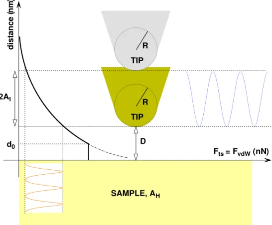
SAMPLE, AH TIP R D d0 TIP R 2A1 Fts = FvdW(nN) distance ( nm )
Figure 3.2: van der Waals forces. The tip oscillates above the sample surface.
The vdW forces for a sphere (tip) with a radius of R and flat (sample) geometry can be obtained from Derjaguin approximation as a function of distance D as
FvdW =
−AHR
6D2 . (3.2)
This equation is valid for D ¿ R [76]. The Hamaker constant (AH) reflects the strength of the vdW forces. AH is a function of the permittivities and refraction indices of tip, sample and the medium in which the interaction takes place. FvdW can be attractive or repulsive depending on the choice of the medium. Hartmann suggested to immerse the tip and sample into a liquid so that the repulsive vdW forces prevent the tip from jumping into contact with the sample [77]. Typically, AH is on the order of 10−19 J in air or vacuum.
a surface. Since the forces are nonlinear, they produce higher harmonics which can be utilized to determine the Hamaker constant. Notice that as D → 0, FvdW → ∞. Therefore below the intermolecular distance d0, the vdW forces are
replaced by the adhesion force in the numerical simulations (see next section).
3.2.1.2 Contact Forces
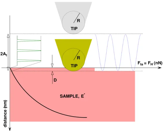
Contact forces include the elastic force and the adhesion force. The elastic force depends on the effective tip-sample elasticity and the adhesion force depends on the work of adhesion. There are several continuum contact theories which relate the applied force to the indentation depth.
• Hertzian mechanics:
This is the simplest theory which does not take the adhesion force into account. According to the Hertzian contact mechanics, the normal load FH is related to the indentation depth D for any kind of indenter as follows [37]
FH = βE∗Dα , (3.3)
where E∗ is the effective Young’s modulus, β and α are the constants dependent on the tip geometry. E∗ is related to the Young’s modulus (E) and Poisson ratio (ν) of the tip and sample:
E∗ = µ 1 − ν2 tip Etip + 1 − ν 2 sample Esample ¶−1 . (3.4)
Mostly, the silicon cantilevers are employed in tapping-mode experiments. Silicon has a high Young’s modulus and the first term in the parenthesis is usually ignored.
Figure 3.3 shows that as the tip hits to the sample, elastic force (pulses) is created. This force and hence its harmonics depend on the sample elasticity. In the case of small harmonic distortion, the tip motion can still be assumed to be sinusoidal.
SAMPLE, E* TIP R D TIP R 2A1 distance ( nm ) Fts = FH(nN)
Figure 3.3: Elastic contact force. The tip touches the sample in a fraction of its oscillation period.
• DMT mechanics:
Unlike the Hertzian theory, DMT (DerjaguMuller-Toporov) mechanics in-cludes the adhesion force. For a sphere-plane geometry, the load is related to the indentation depth as
FDM T = 4 3E
∗√RD3/2− 4πR$ . (3.5)
$ is the adhesion energy per unit area. In the simulations of tapping-mode AFM, generally the DMT mechanics is employed [78–80]. In that case, the adhesion force is equated to the van der Waals forces at the point of contact. Then the interaction force as a function of tip position z can be written as
Fts = −AHR 6z2 for z ≥ d0 −AHR 6d02 +43E∗ √ R(d0− z)3/2 for z ≤ d0 (3.6) where d0 is equal to p
H/(24π$). Note that the slope of the force at d0 is not
continuous.
There are other approaches [81, 82] formulating the load in terms of inden-tation, like BCP (Burnham-Colton-Pollock), JKRS (Johnson-Kendall-Roberts-Sperling), and Maugis mechanics. They are more complex, but they have less deficiencies. In BCP mechanics, e.g., the slope at the point of contact is contin-uous. JKRS and Maugis mechanics include adhesion hysteresis. Since our aim is to show the importance of the higher harmonic imaging in a lucid manner, we will use the Hertzian mechanics in our analysis.
3.2.2
Dissipative Forces
Although not taken into account, it is worth to mention about the dissipative forces which may take place in an experiment. The dissipative forces are the cause of energy dissipation which can be mapped to obtain a material specific image contrast [61].
3.2.2.1 Capillary Forces
The tapping-mode experiments are usually done in air. The ambient humid-ity leads to a thin film of water which covers the tip and sample. As the tip approaches the surface, a meniscus forms upon contact of the adsorbed water layers. When the tip retracts, the capillary neck breaks at a larger distance. This hysteretic behavior results in energy dissipation in each oscillation cycle. The capillary forces can be large enough to obscure vdW forces. Their effect is more sensible on hydrophilic samples than on hydrophobic samples [83].
3.2.2.2 Viscous Forces
Compliant samples, like polymers and biological materials, show viscoelastic be-havior rather than pure elastic or viscous response. Their mechanical bebe-haviors are usually modeled with a parallel combination of a spring and a dashpot (the Voigt model) [84]. The viscous force is proportional to the sample viscosity, ra-dius of the contact area, and tip velocity. Dubourg et al. used tapping-mode AFM to determine quantitatively the viscosity of a triblock copolymer [85].
In addition to capillary and viscous forces, there may be other processes like plastic deformation of the sample, adhesion hysteresis, and mechanical instability of the cantilever which cause energy dissipation.
3.3
Amplitude Damping, Maximum Force and
Contact Time
In tapping-mode operation, as the tip taps on an elastic sample, it indents pe-riodically into the sample during the contact. If we assume that the sinusoidal nature of the tip motion is preserved (low harmonic distortion), then the inden-tation depth is also sinusoidal in the contact duration τ . For a given set point amplitude A1, mean tip to surface separation zr and excitation frequency w, we
can express the time dependent interaction force fTS(t) in one period if |zr| ≤ A1 as fTS(t) = βE∗[A
1cos(wt) − zr]α for |t| ≤ cos−1(zr/A1)/w
0 otherwise
(3.7)
If zr > A1 then fTS(t) = 0 and if zr < −A1 then fTS(t) = βE∗[A1cos(wt) − zr]α. For a cylindrical tip of radius R (β = 2R, α = 1), fTS(t) is a clipped cosine
function for |zr| ≤ A1. Defining a normalized mean tip to surface distance, γ, as
γ = zr/A1, the maximum repulsive force applied to the sample is found to be
Fmax = 2RE∗A1(1 − γ) . (3.8)
In the steady-state, the interaction force can be expanded in a Fourier series [66, 86] as fTS(t) = f0+
P
n≥1fncos(nwt). For |γ| ≤ 1, the average force f0 is given by
f0 = Fmaxξ
sinc(ξ) − γ
1 − γ , (3.9)
where sinc(x) = sin(πx)/(πx). ξ = cos4 −1(γ)/π is the normalized contact time, i.e. contact time divided by one period (wτ /2π). The nth component of the interaction force fn is
fn= Fmaxξgn(γ)/(1 − γ) , (3.10)
where gn(γ) is given by
gn(γ) = sinc[(1 + n)ξ] + sinc[(1 − n)ξ] − 2γsinc(nξ) . (3.11) For n = 1 we get the fundamental component of fTS(t)
f1 = Fmaxξ
1 − sinc(2ξ)
1 − γ . (3.12)
f1 causes an amplitude damping [87] and can be related to oscillation
ampli-tude and cantilever parameters under the assumption of low harmonic distortion as follows
where
ς(w) = {(A0/A1)2− sin2[∠H(w)]}1/2− cos[∠H(w)] , (3.14)
and the transfer function of a fundamental flexural eigenmode of the cantilever is H(w) = Q k (1 − w2/w2 1) Q − iw/w1 (1 − w2/w2 1)2Q2+ w2/w21 , (3.15)
here k, Q, A0 and w1 are the cantilever stiffness, quality factor, free oscillation
amplitude and fundamental resonant frequency, respectively. Equations (3.12) and (3.13) tell us that for any given set of cantilever parameters and a set point amplitude, Fmax and ξ are almost inversely proportional.
A typical tip can be approximated to have a conical shape. In this case, the parameter defining the tip geometry is the semivertical angle θ (β = 2 tan(θ)/π, α = 2). The maximum force applied to the sample is found to be
Fmax = 2 tan(θ)E∗A21(1 − γ)2/π . (3.16)
The average of the interaction force is f0 = Fmaxξ
0.5 + γ2+ 0.5sinc(2ξ) − 2γsinc(ξ)
(1 − γ)2 . (3.17)
The fundamental and higher order force components are found using fn= 2Fmaxξ hn(γ)
(1 − γ)2 , (3.18)
where
hn(γ) = −γ{sinc[(1 + n)ξ] + sinc[(1 − n)ξ]} + (0.5 + γ2)sinc(nξ)
+0.25{sinc[(2 + n)ξ] + sinc[(2 − n)ξ]} . (3.19)
Equations (3.8) and Eq. (3.12) must be satisfied simultaneously for a cylin-drical tip. Similarly, Eq. (3.16) and Eq. (3.18) must be satisfied for a conical tip. We plot Fmax/(βAα1E) and Fmax/f as a function of γ for differing values of E∗ and f1 in Figs. 3.4 and 3.5 for a cylindrical tip and a conical tip. Here, E and
f = βAα
−2 −1.5 −1 −0.5 0 0.5 1 10−2 10−1 100 101 102
Normalized mean tip−surface distance
Normalized maximum applied force
E=100E E=10E E=E E=0.1E E=0.01E f f f f f f * * * * * 1 1 1 =10 =0.1 Cylindrical tip =
Figure 3.4: Normalized maximum repulsive force Fmax/(βAα1E) (thin lines) and
Fmax/f (thick lines) are plotted as a function of normalized mean tip-surface distance γ for varying values of E∗ and f
−2 −1.5 −1 −0.5 0 0.5 1 10−2 10−1 100 101 102
Normalized mean tip−surface distance
Normalized maximum applied force
E=100E E=10E E=E E=0.1E E=0.01E f f f f f f =10 = 0.1 1 1 1 * * * * * Conical tip =
Figure 3.5: Normalized maximum repulsive force Fmax/(βAα1E) (thin lines) and
Fmax/f (thick lines) are plotted as a function of normalized mean tip-surface distance γ for varying values of E∗ and f
1 for a conical tip.
No intersection means that there is no solution for the chosen cantilever. When γ < −1, it is found that f0 = Fmaxγ/(γ − 1), f1 = Fmax/(1 − γ), fn≥2 = 0 for a cylindrical tip and f0 = Fmax(0.5 + γ2)/(1 − γ)2, f1 = −2Fmaxγ/(1 − γ)2,
f2 = 0.5Fmax/(1 − γ)2, fn≥3 = 0 for a conical tip. For a cylindrical tip f1 is
actually equal to 2RE∗A
1, independent of γ. Therefore, there would not be
a damping in the oscillation amplitude as we indent the tip further inside the sample. The only possible solution exists for the sample which gives the effective tip-sample elasticity of f1/2RA1 as Fig. 3.4 shows. For all other samples, there
is an intersection point, unless the tip shape is an infinitely long cylinder. For a conical tip, f1 = −4 tan(θ)E∗A21γ/π increases for decreasing γ and hence there is
In any case, different sample elastic properties give rise to significantly differ-ent Fmax and γ values. Although we are not able to measure any one of these parameters directly [88], we can extract the sample elasticity by measuring the harmonic amplitudes. Notice that the constant term in Eq. (3.7) depends on γ, but the feedback signal contains information on the height variations of the sample surface also.
3.4
Results and Discussion
We can relate the effective tip-sample elasticity to the nth harmonic amplitude for a cylindrical or conical tip by combining Eqs. (3.8),(3.10) or Eqs. (3.16),(3.18) and utilizing An≥2 = |H(nw)fn| as follows
An =
|2RA1H(nw)ξgn(γ)E∗| for a cylindrical tip
|(4/π) tan(θ)A2
1H(nw)ξhn(γ)E∗| for a conical tip
(3.20)
There is no direct relation between Anand E∗ in Eq. (3.20). However, ξ or γ can be used as an independent parameter to find respective An and E∗ values. We can express An and E∗ in terms of γ only
An=¯¯H(nw)A1ς(w)|H(w)|−1Λ(γ)
¯
¯ , (3.21)
where Λ(γ) is equal to gn(γ)/[1 − sinc(2ξ)] for a cylindrical tip and hn(γ)/h1(γ)
for a conical tip. Also E∗ = f
1/[βAα1λ(γ)], where λ(γ) is equal to ξ[1 − sinc(2ξ)]
or 2ξh1(γ) for a cylindrical or conical tip. Notice that as ξ → 0, Λ(γ) → 1 for
which Anreaches its maximum value [max(An)] and λ(γ) → 0 for which E∗ goes to infinity. In Figs. 3.6 and 3.7 we plot first four normalized harmonic amplitudes [An/max(An) = |Λ(γ)|] for cylindrical and conical tips as a function of normalized effective tip-sample elasticity [E∗βAα
1/f1 = λ−1(γ)] under the assumption of a
very small harmonic distortion (An ¿ A1). In these figures, the dashed vertical
line marks the location of a γ = 0 point.
In region I (γ < 0), the tip stays in contact more than a half period. Although we are interested in the solution for region II (γ > 0), we also considered the
100 101 102 103 104 0 0.2 0.4 0.6 0.8 1
Normalized effective tip−sample elasticity
Normalized higher harmonic amplitudes
Region II (0 < < 1) Region I ( < 0) Cylindrical tip 2nd 3rd 4th 5th
γ
γ
|Λ(γ)| 1/λ(γ)Figure 3.6: A variation of the first four normalized harmonic amplitudes |Λ(γ)| as a function of normalized effective tip-sample elasticity λ−1(γ) for a cylindrical tip. It is assumed that An ¿ A1. The vertical dashed line marks the γ = 0
10−1 100 101 102 103 104 105 0 0.2 0.4 0.6 0.8 1
Normalized effective tip−sample elasticity
Normalized higher harmonic amplitudes
2nd 3rd 4th 5th Region II (0 < < 1) Region I ( < 0)
γ
γ
γ
γ
< −1 > −1 |Λ(γ)| 1/λ(γ) Conical tipFigure 3.7: A variation of the first four normalized harmonic amplitudes |Λ(γ)| as a function of normalized effective tip-sample elasticity λ−1(γ) for a conical tip. It is assumed that An ¿ A1. Vertical dashed and dotted lines mark the γ = 0
and γ = −1 locations.
γ < 0 case for the completeness. Region I is further decomposed into two parts as γ < −1 and γ > −1 in Fig. 3.7. Note that the tip can oscillate even if it is fully indented into the sample [89].
The higher harmonic amplitudes show a monotonic increase in a wide range of sample compliance. Notice that the steeply increasing part of the amplitude curves shift towards high Young’s moduli region as the harmonic number in-creases. This makes one of the higher harmonics more preferable than the other ones depending on the sample. As the sample gets stiffer, An saturates since the variation of the contact time (and the penetration depth) gets smaller. This imposes an upper limit for measurable sample elasticity as reported earlier [44].
There is also a lower limit of E∗ for which γ > 0. Both limits can be shifted to the lower side of elasticity by softening the lever, by increasing the set point A1/A0 or oscillation amplitude 1, or by using a dull tip. The use of a dull tip is
not preferable since it decreases the lateral image resolution. There is a practical maximum value of A1/A0 as determined by the precision of the feedback
elec-tronics. The oscillation amplitude can have an upper limit. Hence, the cantilever stiffness is the most suitable parameter to adjust the measurement region. The reverse procedure can be applied to shift the operation range to the high elas-ticity side. Note that changing these parameters also affects the maximum force applied to the surface Fmax. We recall that the surface forces are assumed to be very small (zero) compared to Fmax and increasing Fmax too much can destroy the tip and/or the sample.
Chapter 4
Numerical Analysis for Enhanced
Higher Harmonics
Our analytical analysis proves that the harmonic amplitudes can be utilized for mapping sample elasticity. More generally, it can be used to extract a character-istic of the tip-sample force which may be dominated by any type of interaction. In conventional tapping-mode experiments, on the other hand, the higher har-monics are generally ignored and in fact, their amplitudes are two or three orders of magnitude smaller than the fundamental component of oscillation as both nu-merical [74] and experimental [60] results indicate. The nth harmonic amplitude is related to the nth harmonic of the interaction force fn via the transfer gain |H(nw)| as follows
An = |H(nw)fn| for n ≥ 2 , (4.1)
The transfer function of a rectangular cantilever including higher flexural eigen-modes was obtained by Stark and Heckl [66].
To increase the nth harmonic amplitude Anand hence the measurement sensi-tivity, we must increase either fnor |H(nw)|. Notice that increasing fnmay mean an additional damage to the sample, and therefore it may not be desirable for all kind of samples. The transfer gains for the higher harmonics in conventional tapping-mode operation (w = w1, where w1 is the resonant frequency of the first
mode) are very small unless the higher harmonic frequencies are coincident with the resonant frequencies of the higher eigenmodes. If we consider only the fun-damental eigenmode of a cantilever with stiffness of k, the transfer gain for the nth harmonic will be [k(n2− 1)]−1. This yields a very small value for increasing n. The use of higher harmonics close to the higher transverse resonances can enhance the measurement sensitivity [90]. However, to increase the amplitudes of higher harmonics in this case, one may need to increase the free oscillation amplitude or decrease the set point (damped) amplitude which in turn increases the tip-sample forces.
Most cantilevers do not have eigenmodes at integer multiples of each other. But, it is possible to fabricate special cantilevers, called “harmonic cantilevers”, in such a way that one of the eigenmodes is at an integer multiple of fundamental mode [91]. The recent study by Sahin et al. showed that these cantilevers can be used to enhance one of the higher harmonics [92].
Indeed, measuring the higher harmonic signal sensitively would give an oppor-tunity to researchers in examining the material properties at the nanoscale more effectively. To enhance the quality of the measured harmonic signal, we propose a new method which can easily be employed in conventional tapping-mode systems.
4.1
Higher Harmonic Enhancement
Considering the fundamental eigenmode, the transfer gain reaches its maximum value (Q/k, where Q is the quality factor) at the first resonance frequency w1.
If we drive the cantilever at a submultiple of w1, i.e. at w = w1n = w1/n (n is
an integer number), then, due to the high transfer gain at nw1n = w1, the nth
harmonic amplitude is expected to be much larger than the conventional case. This allows us to detect the harmonic signal with a good signal-to-noise ratio and to inspect the tip-sample interaction effectively. The concept of harmonic enhancement is shown in Fig. 4.1, where the third harmonic is matched to a flexural eigenmode of the cantilever.