Development of a DC fast charging station model for use with EV infrastructure projection tool

Development of a DC Fast Charging Station Model

for use with EV Infrastructure Projection Tool

Emin Y. Ucer

, Mithat C. Kisacikoglu

, Fatih Erden

, Andrew Meintz

and Cl´ement Rames

1_{Dept. of Electrical and Computer Engineering, University of Alabama, Tuscaloosa, AL} 2_{Dept. of Electrical and Electronics Engineering, Bilkent University, Ankara, Turkey}

3_{National Renewable Energy Laboratory, Golden, CO}

eucer@crimson.ua.edu, mkisacik@ua.edu, erden@ee.bilkent.edu.tr, {andrew.meintz,clement.rames}@nrel.gov

Abstract—The deployment of public charging infras-tructure networks has been a major factor in enabling electric vehicle (EV) technology transition, and must continue to support the adoption of this technology. DC fast charging (DCFC) increases customer convenience by lowering charging time, enables long-distance EV travel, and could allow the electrification of high-mileage fleets. Yet, high capital costs and uneven power demand have been major challenges to the widespread deployment of DCFC stations. There is a need to better understand DCFC stations’ loading, utilization, and customer service quality (i.e. queuing time, charging duration, and queue length). This study aims to analyze these aspects using one million vehicle-days of travel data within the Columbus, OH, region. Monte Carlo analysis is carried out in three types of areas - urban, suburban, and rural- to quantify the effect of uncertain parameters on DCFC station loading and service quality.

I. INTRODUCTION

The electric vehicle (EV) market is taking off, with over 500k EVs on the road in the United States and over 2M glob-ally. Although EVs are becoming more popular, the issues that prevent their mass penetration such as limited infrastructure are still present. Replacement of traditional internal combus-tion engine vehicles by EVs goes hand-in-hand with the mass deployment of reliable and fast charging infrastructure.

The National Renewable Energy Laboratory (NREL) to-gether with the California Energy Commission (CEC) devel-oped the Electric Vehicle Infrastructure Projection Tool (EVI-Pro) to estimate regional requirements for charging infrastruc-ture to support consumer adoption of EVs [1], [2]. EVI-Pro utilizes EV market and real-world travel data to estimate future requirements for home, workplace, and public charging infrastructure [1], [2].

There are two types of EV charging methods: (i) on-board charger for AC grid connection which can be single-phase L1 and L2 as defined in SAE J1772, and three-phase AC charging as defined in SAE J3068 (work in progress); and (ii) DC fast charging (DCFC) as defined in SAE J1772-Combo/CHAdeMO standards. L1 and L2 are mostly located at residential and

public/workplace charging premises. These stations do not include a power electronics converter but rather utilize the vehicle’s on-board charger which is rated at low power levels (typically less than 19.2 kW) [3]. On the other hand, DCFC stations operate at high power DC voltage and use an off-board AC-DC converter [3]. Thus, they provide much higher charging power level compared to L1 and L2. In this study, we will focus mainly on development and analysis of the DCFC infrastructure model.

There are several important points that should be addressed regarding the installation of DCFC stations: their locations, operation costs, and how to evaluate the service quality [4]. DCFC geographic location has to be close to where it is needed and should ensure relatively high mobility of EVs [4]. Berjoza and Jurgena [4] proposed a simple algorithm for calculating the characteristics of charging stations. This algorithm deter-mines metrics like the availability ratio for charging stations. Zenginis et al. [5] describe a novel queuing model where the customers’ mean waiting time is computed by considering the available charging spots, arrival process, and charging needs of various vehicle classes. Quality of service (QoS) is measured by waiting time of the customers in the queue prior to charging their EVs. Various EVs are classified by their battery size, and customers’ mean waiting times in the queue are computed by considering the available charging spots and stochastic arrival process and charge needs of the various EV classes.

Fan et al. [6] studies the impact of the requested state of charge (SOC) of EVs on charging times and proposes an operation analysis of fast charging stations where operators can set a limit on the requested SOCs to obtain maximized revenue.

This study develops an analysis of DCFC power consump-tion based on data provided by EVI-Pro. One million vehicle-days of travel from the Columbus, OH, region – the winner of the U.S. Department of Transportation’s Smart City award – were simulated in EVI-Pro to generate about 23k DCFC events. Monte Carlo (MC) simulations are carried out to predict the charging load and queuing time at three stations – in urban, suburban and rural settings.

The organization of the paper is as follows. Section II presents the data collected from EVI-Pro. Section III describes

the development of the DCFC station model. Section IV focuses on the MC simulation set-up, and Section V describes the results. Finally, Section VI concludes the study.

II. DATACOLLECTIONMETHODOLOGY ANDEVI-PRO

MODEL

EVI-Pro anticipates spatially and temporally resolved con-sumer charging demand while capturing variations with re-spect to residents of single-unit dwellings (SUDs) and multi-unit dwellings (MUDs), weekday/weekend travel behavior, and regional differences in travel patterns and vehicle adop-tion. To identify the optimal charging strategy, individual travel days from a travel data set (originally completed using a conventional gasoline vehicle) are simulated in EVI-Pro under different assumptions for charging infrastructure availability. This model only considers destination charging as opposed to en-route charging between destinations.

The modeled vehicle fleet consists of both plug-in hybrid (PHEVs) and battery electric vehicles (BEVs), but only BEVs are eligible to use DCFC stations. The default charging be-havior is “home-dominant,” meaning that consumers prefer to charge at their residence, then at their workplace, and finally in public locations. This charging demand simulation generates a set of charging sessions required to satisfy the travel pat-terns displayed in the data in a way that maximizes electric miles traveled and minimizes operational cost. These charging sessions are then post-processed spatially and temporally to output electric vehicle supply equipment (EVSE) requirements and station utilization for the Columbus region. More detail on this methodology can be found in [7].

EVI-Pro relies on real-world travel data to simulate EV charging demand. A large, commercial data set was procured from INRIX [8], consisting of GPS travel trajectories (mode imputed as driving trips by INRIX) that intersected the Colum-bus, OH, region in 2016. Each trajectory features trip-level data such as start/end times and GPS coordinates (including origins, destinations, and intermediate way points). The full data set was down selected to include only light-duty consumer vehicle GPS data collected from mobile/cellular devices. A thorough data cleansing routine was applied to ensure the integrity of travel days simulated in EVI-Pro. The cleansed input data set includes approximately 1.02 million full travel days, 3.71 million trips, and 30.6 million miles of driving.

The results of these simulations show that the majority of charging required to satisfy travel needs of drivers from the INRIX data set can be accommodated with residential charging. However, some DCFC is required to accommodate high vehicle miles traveled (VMT), short dwell time travel days. The simulation generated about 23,600 DCFC events across the Columbus region, with the highest density (just over half of all events) occurring in Franklin County, 30% occurring in the six neighboring counties, and the remaining 20% scattered across the rest of Ohio and the Midwest. These charging events are clustered into 400 DCFC stations, flagged as urban (Franklin County), suburban (six neighboring counties), and rural (outside of the Columbus metro area). The

Figure 1: Map of station locations and charging events in Colombus, OH (Blue: urban, green: suburban, magenta: rural).

Figure 2: Structure of the DCFC station model and EVI-Pro interaction.

map of all stations are shown in Fig. 1. The size of the circles is proportional to the number of charging sessions, and the colors represent the three zones.

III. DEVELOPMENT OF THEDCFC STATIONLOADMODEL

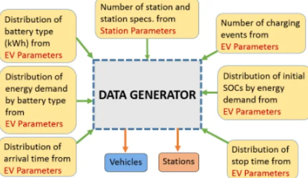
Fig. 2 shows the structure of the interaction between the developed DCFC station model and EVI-Pro. EVI-Pro provides the necessary input data and stochastic mobility parameter distributions to the DCFC station model which in turn generates vehicle charging events and stations. The input data provided by EVI-Pro can be divided into three categories: (i) station parameters, (ii) vehicle parameters, and (iii) station use parameters.

Station parameters include number of stations, their capac-ities, number of ports, and port capacities. Vehicle parameters define vehicle types, battery sizes, maximum charging powers, and charge acceptance curves. The data also provide several distributions for vehicle types, arrival times, energy demands, and initial SOCs along with number of charging events at each station. A brief overview of the variable generation process is shown in Fig. 3.

In order to understand the design criteria for a DCFC station, it is necessary to develop the likelihood of all possible

Figure 3: Structure of data generation.

outcomes and the risks these represent. The MC analysis is an effective tool for this purpose. It provides possible outcomes and also their associated probabilities bringing a broader view of what might happen. For this purpose, we utilized MC analysis by running 10 monthly simulations with the same input data. At each run, vehicle related parameters such as time of arrival, energy demand, initial SOC, etc. are randomly regenerated from the associated probability density functions (PDFs). During the simulations, vehicles arrive at the corresponding stations, wait in the queue (if there is not any available port), are plugged in, and then charged according to their charge acceptance curves. They depart after their energy demand is met, and a new vehicle from the queue is plugged into an available port.

IV. SIMULATIONSET-UP

This section defines the simulation parameters and presents the results. The following are the defined parameters for the simulations, stations, and vehicles.

Simulation parameters:

• Number of MC simulations: 10

• Single simulation duration: 4 weeks (1-min resol.) Station parameters (Urban, Suburban, Rural):

• Number of stations: 3

• Number of ports of each station: [12, 4, 1]

• Station capacities: [1800, 600, 50] kW

• Port capacities: [150, 150, 50] kW Vehicle parameters:

• Number of vehicle types: 3

• Battery sizes: [24, 60, 85] kWh

• Max. SOC limit: [80, 80, 80] %

• EV-type probability distributions – Station 1: [0.8900, 0.0503, 0.0598] – Station 2: [0.8513, 0.0691, 0.0796] – Station 3: [0.6403, 0.1675, 0.1922]

• Vehicle set-up time: 5 min

The charge acceptance curves for these vehicle types are given in Fig. 4. This figure shows how the charging power of vehicle batteries vary as a function of battery SOC. The curves for each vehicle type were developed based on DCFC data acquired from a 2012 Nissan LEAF [9]. This charging power data are collected after a full vehicle thermal soak to

Figure 4: Charge acceptance curves for three vehicle types with Nissan LEAF fast charging data.

allow the battery to reach 25◦C. The vehicle data are included in Fig. 4 and are for a charge from about 15% to 90% SOC. A curve-fit method is used to define the charge acceptance curve at intervals of 2.5% SOC for the 24 kWh vehicle type. The remaining charge acceptance curves are determined assuming a cell-level charge power decrease of 60% in the power-to-energy (P-E) ratio that is then scaled for the larger capacity 60 kWh and 85 kWh vehicle types. The decrease in P-E is used to account for the use of more energy dense cells in the production of longer range vehicles [10], [11].

These charge acceptance curves are used by the DCFC model to limit the charge power to the charging vehicles based on their SOC throughout the fast charge. Thermal and time-dependent charge diffusion limitations on charging power have not been accounted for in this model. The charge data from the Nissan LEAF demonstrate a simplified constant-current charging method up to 60% SOC and a then constant-voltage methodology to higher SOCs. While the SOC transition to constant-voltage may vary depending on battery chemistry and other more aggressive charging methods have been proposed [12] [13], this approach provides an approximation of the battery limitations on charge power. The impact to the DCFC station of these advanced charging strategies are left for future work.

To demonstrate how a charging event takes place, the charging profiles of three different types of vehicles (with 24, 60 and 85 kWh battery sizes) are presented in Figs. 5– 7, respectively. The vehicles are randomly selected out of approximately 23k charging events. In these figures, one can observe when the vehicles arrived at the stations, whether or not they had to wait in a queue (none of them entered the queue in the presented cases), its set-up time, and when its charging started. Further, one can observe how EVs’ charging power changed over time as a result of charge acceptance rate, how their SOC changed, and when they finished with charging and departed.

Figure 5: Charging profile of a 24 kWh vehicle.

Figure 6: Charging profile of a 60 kWh vehicle. V. RESULTS ANDANALYSIS

The simulations were run with the parameters defined above for a station design in each region using the average number of charge events of the stations in the respective region. Table I gives the statistical results of all MC simulations for each station. Four criteria have been chosen for analysis and comparison: 15-min average power consumption of the stations (termed as ”demand power” in this study), charging duration statistics at each station, queuing statistics (queuing duration and queue length), and port usage. Table I can help draw important conclusions regarding the load profile, QoS, and effective use of available power at the station. As an example, an increase in average and peak demand power and a decrease in the queuing durations can be noted from station 3 to station 1 due to increased power capacities and port numbers. Further, maximum power consumption of station 1 is almost a third of the station total capacity. However, the same station experiences a maximum queuing duration as high as 12 min.

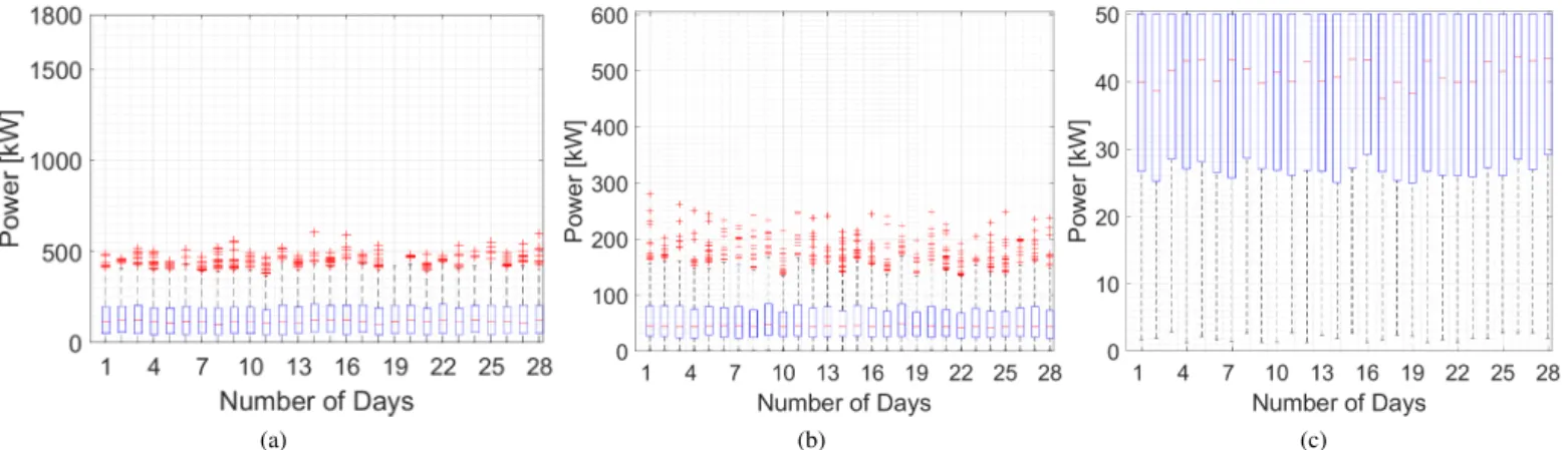
Demand charges can be as high as 90% of electricity costs of a DCFC station according to a recent report [14]. Therefore, demand power consumption of different DCFC station types are explained using box plots. Fig. 8 shows the box plots of demand power consumption of the stations for each day after 10 MC simulations. Bottom and top lines of each box represent 25th _{and 75}th_{percentile of all samples, respectively.}

Figure 7: Charging profile of a 85 kWh vehicle. Straight lines in each box refer to median of all samples. Maximum limit of the dotted lines (>) cover the 99.3%, and the remaining red outliers (+) fall into 0.7% of all samples.

Even though the total capacities of stations 1 and 2 are 1,800 kW and 600 kW, respectively, 75th _{percentile of all}

power consumptions fall well below their rated capacity with the outlier events below half of the rated power. The peak demand power for station 1 designated by the outliers is around one-third of the station’s rated capacity. This ratio is a little higher for station 2, indicating that the capacity of station 2 is more effectively used. Station 3, on the other hand, uses all of its capacity every day since it has only one port. This means that either or both a capacity increase and port count increase for this station should be considered.

Fig. 9 shows the probability histograms of the demand power consumption for all time at each station for 10 MC simulations. These figures show the likelihoods of total power consumptions that the stations will have to handle. As seen, the figures are consistent with the statistical results presented in Table I.

Fig. 10 corresponds to the percent of station port utilization. ”0 port” indicates the times when no EVs are present at the station. This figure reveals that 70% of the time, the ports of station 3 are not utilized. Therefore, adding an additional port may not make a big difference in terms of meeting the demand of the station. Instead, a station with a higher port capacity would reduce the duration of the charge events and could better improve queuing duration and length.

Table I: Important statistical results of MC simulations.

Station Details Station 1 Station 2 Station 3 Station port count 12 4 1 Station power capacity (kW) 1800 600 50 Monthly charging events 3976 896 308 Charging Aver. demand power (kW) 136.26 55.19 36.59 Power Max. demand power (kW) 606.58 279.83 50 Charging Max. charging dur. (min) 54 54 91 Duration Aver. charging dur. (min) 20.73 21.73 35.14

Min. charging dur. (min) 8 8 8 Queuing

Max. queuing dur. (min) 12 30 276 Aver. queuing dur. (min) 0.04 0.25 30.14 Max. queue length (# EV) 5 5 7 Aver. queue length (# EV) 0.004 0.006 0.230 Port Max. port util. (# ports) 12 4 1 Utilization Aver. port util. (%) 30.8 39 100

(a) (b) (c)

Figure 8: Demand power boxplots of stations (a) #1, (b) #2, and (c) #3.

(a) (b)

(c)

Figure 9: Demand power probability histograms of stations (a) #1, (b) #2, and (c) #3 (No EV case excluded).

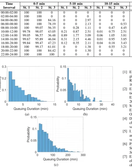
The queue at the station is another important parameter that results in extra waiting times and decreases QoS. The average and maximum queue length and queuing durations among all MC simulations for each station in a month were already given in Table I. Fig. 11 shows the probability of queuing durations at each station for the customers that happened to wait in the queue excluding zero waiting times. This provides better information on the queuing time spectrum. Further, the probabilities of waiting in different time intervals in a day are also calculated. The results are presented for different waiting times as a probability chart in Table II. It shows the probability of how long a user will wait in the queue at each station at any time of the day. As the queue length increases, the waiting times will increase and QoS will decrease. Since Station 1 offers charging at higher powers and has more ports, it is very unlikely to wait more than 10 min at this station. The worst case scenario happens for Station 3 where the probability of

0port 1port 2ports 3ports _{4ports ≥5ports} 0 20 40 60 31 17 11 _{9 8} 24 62 22 10 4 ₂ 70 30 Port Utilization %

Station#1 Station#2 Station#3

Figure 10: Port utilization of each station.

waiting more than 25 min in the queue between 12:00-14:00 is 37%. This also follows the statistical results in Table I that show the average waiting duration for Station 3 is 30 min. This is definitely not a reasonable risk for the station operator since it clearly loses potential customers to other stations. To overcome this problem, either the power capacity of the available port/station or installing an additional port should be considered.

VI. CONCLUSIONS ANDFUTUREWORK

In this work, we developed a DCFC station model and analyzed three different DCFC stations using charging data acquired from EVI-Pro. The model ran a thorough analysis on DCFC station operation to understand statistical metrics such as peak demand power, customer service quality, and port utilization. While the increased station power capacity and port number result in a higher peak demand power, it is very dependent on EV charge acceptance. Further, increasing port number increases customer QoS but decreases port utilization. As an example, an 1,800 kW, 12-port DCFC resulted in a 33.7% peak loading and 30.8% port utilization. The probability of waiting more than five minutes in the queue at this station is at worst 0.95% during a day. Future study will focus on optimum decision making of station capacity and port number as well as investigating charge control algorithms to respond to grid commands.

Table II: Probability of queuing duration for three stations at different times of day (%).

Time 0-5 min 5-10 min 10-15 min 15-20 min 20-25 min >25 min Inverval St. 1 St. 2 St. 3 St. 1 St. 2 St. 3 St. 1 St. 2 St. 3 St. 1 St. 2 St. 3 St. 1 St. 2 St. 3 St. 1 St. 2 St. 3 00:00-02:00 100 100 0 0 0 0 0 0 0 0 0 0 0 0 0 0 0 0 02:00-04:00 100 100 0 0 0 0 0 0 0 0 0 0 0 0 0 0 0 0 04:00-06:00 100 100 84.16 0 0 2.97 0 0 0 0 0 0.99 0 0 0 0 0 10.89 06:00-08:00 100 100 78.19 0 0 2.13 0 0 0.53 0 0 1.06 0 0 2.13 0 0 15.43 08:00-10:00 100 99.07 56.35 0 0.28 1.11 0 0.47 4.45 0 0.19 2.67 0 0 3.12 0 0 28.29 10:00-12:00 99.78 98.07 43.05 0.21 0.87 2.51 0.01 0.75 2.51 0 0.25 3.18 0 0.06 4.52 0 0 34.34 12:00-14:00 99.05 96.57 36.48 0.89 1.77 3.09 0.06 1.05 3.81 0 0.39 2.18 0 0.22 2.54 0 0 37.75 14:00-16:00 99.67 95.89 46.04 0.31 2.15 4.46 0.01 0.95 3.85 0 0.7 4.26 0 0.19 3.85 0 0.13 27.18 16:00-28:00 99.84 99.47 47.23 0.12 0.35 2.11 0.04 0.18 3.43 0 0 5.28 0 0 1.85 0 0 29.02 18:00-20:00 100 99.17 61.01 0 0 1.38 0 0.55 3.21 0 0 3.21 0 0.28 4.59 0 0 22.48 20:00-22:00 100 100 84.42 0 0 1.30 0 0 0 0 0 2.60 0 0 2.60 0 0 5.19 22:00-24:00 100 100 100 0 0 0 0 0 0 0 0 0 0 0 0 0 0 0 (a) (b) (c)

Figure 11: Queuing duration probabilities for stations (a) #1, (b) #2, and (c) #3. (zero queuing time excluded)

VII. ACKNOWLEDGEMENT

This work was supported by the U.S. Department of Energy under Contract No. DE-AC36-08GO28308 with the National Renewable Energy Laboratory. This report and the work described were sponsored by the U.S. Department of Energy (DOE) Vehicle Technologies Office (VTO) under the Systems and Modeling for Accelerated Research in Transportation (SMART) Mobility Laboratory Consortium, an initiative of the Energy Efficient Mobility Systems (EEMS) Program. The authors acknowledge John Smart of Idaho National Laboratory for leading the Alternative Fueling Infrastructure Pillar of the SMART Mobility Laboratory Consortium. The following DOE Office of Energy Efficiency and Renewable Energy managers played important roles in establishing the project concept, advancing implementation, and providing ongoing guidance: David Anderson, Sarah Olexsak, and Rachael Nealer.

The U.S. Government retains and the publisher, by ac-cepting the article for publication, acknowledges that the U.S. Government retains a nonexclusive, paid-up, irrevocable, worldwide license to publish or reproduce the published form of this work, or allow others to do so, for U.S. Government purposes.

REFERENCES

[1] E. Wood, S. Raghavan, C. Rames, J. Eichman, and M. Melaina, “Re-gional charging infrastructure for plug-in electric Massachusetts,” Nat. Renewable Energy Lab. (NREL), Golden, CO, Tech. Rep. DOE/GO-102016-4922, 2017.

[2] E. Wood, C. Rames, M. Muratori, S. Raghavan, and M. Melaina, “Na-tional plug-in electric vehicle infrastructure analysis,” Nat. Renewable Energy Lab. (NREL), Golden, CO, Tech. Rep. DOE/GO-102017-5040, 2017.

[3] M. C. Kisacikoglu, A. Bedir, B. Ozpineci, and L. M. Tolbert, “PHEV-EV charger technology assessment with an emphasis on V2G operation,” Oak Ridge Nat. Lab., Tech. Rep. ORNL/TM-2010/221, Mar. 2012. [4] D. Berjoza and I. Jurgena, “Analysis of distribution of electric vehicle

charging stations in the Baltic,” Engineering for Rural Development, vol. 14, no. January, pp. 258–264, 2015.

[5] I. Zenginis, J. S. Vardakas, N. Zorba, and C. V. Verikoukis, “Analysis and quality of service evaluation of a fast charging station for electric vehicles,” Energy, vol. 112, pp. 669–678, 2016.

[6] P. Fan, B. Sainbayar, and S. Ren, “Operation Analysis of Fast Charging Stations With Energy Demand Control of Electric Vehicles,” IEEE Trans. Smart Grid, vol. 6, no. 4, pp. 1819–1826, 2015.

[7] E. Wood, C. Rames, M. Muratori, S. Raghavan, and S. Young, “Charging electric vehicles in smart cities: An EVI-Pro analysis of columbus, ohio.” Nat. Renewable Energy Lab. (NREL), Golden, CO, Tech. Rep. NREL/TP-5400-70367, 2017.

[8] INRIX, “INRIX: Intelligence that moves the world,” http://inrix.com/ about/, [Online; accessed 20-Nov-2017].

[9] Idaho Nat. Lab., “2013 Nissan Leaf: Advanced vehicle testing tivity,” https://avt.inl.gov/vehicle-button/2013-nissan-leaf, [Online; ac-cessed 24-Nov-2017].

[10] General Motors, “Drive unit and battery at the heart of Chevrolet Bolt EV, press release,” http://media.gm.com/media/cn/en/gm/news.detail. html/content/Pages/news/cn/en/2016/jan/0114 bolt-ev.html, [Online; ac-cessed 24-Nov-2017].

[11] Nissan Motor Co., “Electric vehicle lithium-ion battery Nissan technological development activities,” http://www.nissan-global.com/en/ technology/overview/li ion ev.html, [Online; accessed 24-Nov-2017]. [12] R. Klein, N. A. Chaturvedi, J. Christensen, J. Ahmed, R. Findeisen,

and A. Kojic, “Optimal charging strategies in lithium-ion battery,” in American Control Conf. (ACC), 2011, pp. 382–387.

[13] Y.-H. Liu, J.-H. Teng, and Y.-C. Lin, “Search for an optimal rapid charging pattern for lithium-ion batteries using ant colony system algorithm,” IEEE Trans. Ind. Electron., vol. 52, no. 5, pp. 1328–1336, 2005.

[14] G. Fitzgerald and C. Nelder, “EVgo fleet and tariff analysis,” Rocky Mountain Inst., Tech. Rep., 2017.