Fast algorithms for linear and nonlinear microwave circuit simulation

(1)

?, у-;Ч i л , ί'.;·. .■ ·; ■ ; './ ■· : - ΐ.Γ’· . . · ί··*'· ί"· ?·■ ■. ■; ' .>> 1 '^! I -Γ 'ί ié ѴІ · i ^ Ü ύ ‘- ι ^ i Ш Ч < * r # ^ W - W we*^ t « *· » Щ » - i ¿ w ІІ* W ; W - « Н ^ v ' J ' ' ¿ ' Í J ¿ Ч«г· V i ¿ ¿ •4 ; . ' f · ^ · ’ /ч\. . ѴѴо> · , r — <; , re · * · 'іИв ^<^JL

(2)

PAST ALGORITHMS FOR LINEAR AND NONLINEAR

MICROWAVE CIRCUIT SIMULATION

A DISSERTATION

SUriMITTED TO THE DEPARTMENT OF ELECTRICAL AND ELECTRONICS ENGINEERING

AND THE INSTITUTE OF ENGINEERING AND SCIENCE

OF BILKENT UNIVERSITY

IN PARTIAL FULFILLMENT OF THE REQUIREMENTS

FOR THE DEGREE OF

DOCTOR OF PHILOSOPHY

By

Mustafa Çelik

July 1994

(3)

I certify that I have read this thesis and that in my opinion it is fully adequate, in scope and in quality, as a dissertation for the degree of Doctor of Philosophy.

/"

Abdullah Atalar, Ph. D. (Supervisor)

M. Ali Tan, Ph. D. (Co-supervisor)

(4)

ГК

- С 4 5 ^ЭЭ4

(5)

I certify that I have read this thesis and that in iny opinion it is fully adequate, in scope and in quality, as a dissertation for the degree of Doctor of Philosophy.

L

M. ir§adi Aksun, Ph. D.

Cemal Yalabık, Ph. D.

Murat A§kar, Ph. D.

Approved for the Institute of Engineering and Science:

Mehmet Baray,

(6)

(7)

Abstract

FAST ALGORITHMS FOR LINEAR AND NONLINEAR

MICROWAVE CIRCUIT SIMULATION

Mustafa Çelik

Ph. D. in Electrical and Electronics Engineering

Supervisors:

Prof. Dr. Abdullah Atalar and Assoc. Prof. Dr. M. Ali Tan

July 1994

A new method is proposed for dominant pole-zero (or pole-residue) analysis of large linear microwave circuits containing both lumped and distributed elements. This method is based on a multipoint Fade approximation. It finds a reduced order rational s-domain transfer function using a data set obtained by solving the circuit at only a few frequency points. We propose two techniques in order to obtain the coefficients of the transfer function from the data set. The proposed method provides a more efficient computation of both transient and frequency domain responses than conv'entional simulators and more accurate results than the techniques based on single-point Fade approximation such as Asym ptotic Waveform Evaluation.

This study also describes a new method for the transient analysis of large circuits containing weakly nonlinear elements, linear lumped components, and the linear elements specified with frequency domain parameters such as lossy multiconductor transmission lines. The method combines the Volterra-series technique with Asymptotic Waveform Evaluation approach and corresponds to recursive analysis of a linear equivalent circuit.

(8)

We have also proposed a new method to find steady state responses of nonlinear microwave circuits. It is a modified and more efficient form of Newton-Raphson iteration based harmonic balance (HB) technique. It solves the convergence problems of the HB technique at high drive levels. The proposed method makes use of the parametric dependence of the circuit responses on the excitation level. It first computes the derivatives of the complex amplitudes of the harmonics with respect to the excitation level efficiently and then finds the Fade approximants for the amplitudes of the harmonics using these derivatives.

K e y w o r d s : Microwave circuit simulation, Fade approximation, pole-zero computa tion, transient analysis, Volterra-series, steady state analysis, harmonic balance technique.

(9)

özet

DOĞRUSAL V E DOĞRUSAL O LM AYAN M İK RO D ALG A D EVR E

BEN ZETİM İ İÇİN HIZLI A L G O R İT M A L A R

Mustafa Çelik

Elektrik ve Elektronik Mühendisliği Doktora

Tez Yöneticileri:

Prof. Dr. Abdullah Atalar ve Doç. Dr. M. Ali Tan

Temmuz 1994

Hem toplu hem dağıtılmış ögeli eleman içeren büyük doğrusal mikrodalga devrelerin sıfır- kutup (kalmtı-kutup) analizi için yeni bir yöntem önerilmiştir. Yöntem cok noktalı Pade yaklaşımına dayanmaktadır. Devrenin sadece birkaç frekans noktasında çözülmesiyle elde edilen bir veri kümesi kullanılarak düşük dereceli bir rasyonel aktarım foksiyonu bulunur. Önerilen yöntem, geleneksel benzeticilerden daha verimli, asimtotsal eğri bulma gibi tek noktalı Pade yaklaşımına dayanan tekniklerden de daha doğru bir frekans ve zaman yanıtı hesaplanmasına olanak verir.

Bu tezde ayrıca çok sayıda doğrusal toplu ögeli eleman ve yitimli çok-iletkenli iletim hattının yanında az sayıda da yumuşak huylu doğrusal olmayan sonlandırıcı içeren devrelerin geçici durum analizi için yeni bir metot önerilmiştir. Bu metot Volterra-dizisel tekniğini asimtotsal eğri bulma yaklaşımıyla birleştirir ve doğrusal denk bir devrenin özyineli bir şekilde analizine karşılık gelir.

Bu çalışmada ayrıca doğrusal olmayan mikrodalga devrelerin kalıcı durum analizi için

(10)

yeni bir metot önerilmiştir. Önerilen metot, Newton-Raphson dürüme dayalı katsıklık denge tekniğinin daha verimli ve değiştirilmiş bir biçimidir ve katsıklık denge tekniğinin yüksek sürüş seviyelerindeki yakınsama sorunlarını çözer. Bu metot devre yanıtlarının sürüş seviyesine olan parametrik bağlılığını kullanır. İlk önce katsıklık bileşenlerinin sürüş seviyesine göre türevleri verimli bir şekilde hesaplanır, daha sonra da bu türevler kullanılarak katsıklık bileşenleri için Pade yaklaşımları bulunur.

A n a h ta r S özcü k ler: Mikrodalga devre benzetimi, Pade yaklaşımı, sıfır-kutup hesabı, geçici durum analizi, Volterra-dizisi, kalıcı durum analizi, katsıklık denge tekniği.

(11)

Acknowledgment

I would like to thank Dr. Abdullah Atalar and Dr. M. Ali Tan, iny thesis supervisors, for their help and guidance during the preparation of this thesis. It hais been an honor and a pleasure to work with them. I am particularly indebted to Dr. Atalar who encouraged me to work on circuit simulation.

I would like to express my thanks to Dr. M. Irşadi Aksun and Ogan Ocali for many valuable discussions and suggestions during the course of this work. I would also like to thank my colleague Satılmış Topçu.

I like to acknowledge the financial support of NATO through SFS project (TU- MIMIC).

(12)

Abstract i Ozet iii Acknowledgment v Contents vi List of Figures ix List of Tables xi 1 Introduction 1 1.1 Dominant pole-zero c o m p u t a t io n ... 1 1.2 Transient analysis of weakly nonlinear c ir c u it s ... 4 1.3 Steady-state analysis of nonlinear circu its... 6

2 Model Reduction Using Fade Approximation 8

2.1 Model reduction... 8 2.2 Asymptotic Waveform E valu ation... 9 2.2.1 Complex Frequency H opping... 11

(13)

3 Model Reduction Using Multipoint Fade Approximation 14

3.1 Frequency Shifted M o m e n t s ... 14

3.2 Multipoint Moment M a tc h in g ... 15

3.2.1 Method 1 ... 16

3.2.2 Method 2 ... 18

3.3 Practical C on sid era tion s... 20

4 Evaluation of the Moments for Microwave Circuits 24 4.1 Circuit Form ulation... 24

4.2 Moments of the Blocks Characterized by Measured D a t a ... 27

4.3 Moments of the Transmission L in e s ... 29

4.3.1 ТЕМ and Quasi-TEM Transmission L i n e s ... 29

4.3.2 Transmission Lines with Full-wave Analysis ... 34

5 Applications in Linear Microwave Circuits 37 .5.1 Frequency re s p o n s e ... 37

5.2 Transient response ... 38

5.3 E x a m p le s ... 39

6 Transient Response of Circuits With Weakly Nonlinear Terminations 51 6.1 The Volterra S e r ie s ... 51

6.2 Circuit form u la tion ... 52

6.3 Finding the Volterra responses... 53

(14)

6.3.1 Finding the source v e c t o r s ... 54

6.3.2 Finding the transient response of the linearized circuit 56 6.4 A lg o r ith m ... 57

6.5 E x a m p le s ... 58

7 A New Method for the Steady-State Analysis of Nonlinear Circuits 63 7.1 The Harmonic Balance A p p r o a c h ... 63

7.1.1 Circuit form u la tion ... 63

7.1.2 Harmonic Balance T e c h n iq u e ... 64

7.1.3 Newton-Raphson m eth od ... 65

7.2 Proposed m e t h o d ... 67

7.2.1 Computation of the D e riv a tiv e s... 68

7.2.2 Computation of the Source V e c t o r s ... 71

7.2.3 Approximating the Fourier C oefficien ts... 72

7.2.4 The A l g o r i t h m ... 73

7.3 E x a m p le s ... 74

8 Conclusions 80 8.1 S u m m a r y ... 82

(15)

List of Figures

2.1 Determination of accurate p o l e s ... 13

4.1 Example c ir c u it ... 31

4.2 Frequency response com parison... 33

4.3 The microstrip s tru c tu re ... 36

5.1 Piecewise linear fu n c tio n ... 39

5.2 Frequency response (magnitude) comparison for the amplifier circuit. . . . 40

5.3 Frequency response (phase) comparison for the amplifier circuit... 41

5.4 Low-pass filter... 41

5.5 Frequency response of the low-pass f i l t e r ... 42

5.6 Step response of the low-pass filter ... 43

5.7 Normalized error in the frequency respon se... 45

5.8 Interconnect c ir c u it ... 46

5.9 Frequency response of the interconnect c i r c u i t ... 47

5.10 Normalized errors in the frequency r e s p o n s e ... 47

5.11 Step response of the interconnect c i r c u i t ... 48

(16)

5.12 Errors in the step r e s p o n s e s ... 48

5.13 Frequency (magnitude) response of the band-pass f i l t e r ... 49

5.14 Frequency (phase) response of the band-pass filt e r ... 50

5.15 Step response of the band-pass filter ... 50

6.1 Nonlinear c o n d u c ta n c e ... 55

6.2 Circuit for Example 1 ... 58

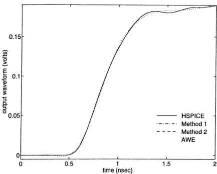
6.3 The output voltage waveform for example # 1 ... 59

6.4 First, third, fifth, and eleventh order outputs for example # 1 59 6.5 Cii'cuit for example 2 ... 60

6.6 The output voltage waveform for example ^ 2 ... 61

6.7 Circuit for Example 2 ... 62

6.8 First, second, fourth and sixth order outputs and resulted output waveform for the circuit of Example 2 ... 62

7.1 Doubler c i r c u i t ... 74

7.2 Powers of the harmonics at the lo a d ... 75

7.3 Harmonic balance error vs input power(ei = 10“ ®, t2 = 10“ ^)...75

7.4 Comparison of number of Newton-Raphson ite ra tio n s... 76

7.5 Comparison of Fade and polynomial approximations for dc component . . 77

7.6 Comparison of Fade cind polynomial approximations for the first harmonic 77 7.7 Mesfet (nonlinear equivalent) circuit ... 78

7.8 Powers of the harmonics at the lo a d ... 79

7.9 Harmonic balance error vs input power(ci = 10“ "*, ¿2 = 10“ ® ) ... 79

(17)

List of Tables

5.1 Approximated poles obtained from the proposed method and the Complex Frequency Hopping technique for the low-pass filter... 44

(18)

Chapter 1 Introduction

With the increasing complexities of modern microwave circuits, computer-aided design (CAD) tools have become an essential tool for microwave circuit designers. Although, some of the CAD programs have been around for almost three decades, there is an increased demand for more accurate and faster CAD tools because of the rapid increase in operating frequencies and decrease in feature size.

This study deals mainly with the analysis or in other words simulation part which is the most important component of the microwave CAD. In this thesis we propose some methods which are either faster or more accurate or both faster and more accurate than the existing circuit simulation algorithms.

This thesis contains three parts. These are, i) analysis of linear circuits, ii) transient analysis of weakly nonlinear circuits, and iii) steady-state analysis of nonlinear circuits.

1.1 Dominant pole-zero computation

In order to analyze linear circuits, obtaining the pole-zero information is sufficient because it provides the circuit response both in time and frequency domain. It also gives insight for the design process.

(19)

Pole-zero computation in a linear circuit is algebraically equivalent to the computation of the eigenvalues of a circuit matrix. There exist many numerical eigenvalue algorithms including QR, QZ, deflation-QZ, Muller, MD-QR algorithms. Pole computation routines based on the Muller algorithm have been incorporated in recent versions of SPICE [1] [2]. A detailed comparison of the numerical eigenvalue algorithms for pole-zero computation is given in Ref. [3].

Another approach in pole-zero computation is to obtain a rational network function in the s-domain and find the poles and zeros from the polynomials of this rational function by means of a standard root finding algorithm. A review of symbolic frequency domain network analysis methods can be found in Ref. [4]. Among these methods the most popular one is the numerical interpolation method which is based on polynomial interpolation with arbitrary selection of frequency points. It is shown in Ref. [5] that the best result is obtained when the interpolation points are uniformly distributed on the unit circle, which is known as interpolation using FFT algorithm. Most of the symbolic analysis methods, including the interpolation algorithm, try to compute an exact form of the network functions in the frequency domain.

The methods mentioned above are not practical for microwave circuits for two reasons:

1. Usually, practical microwave circuits are of large size, therefore difficult to analyze. Even a simple circuit may have a very large equivalent circuit due to highly complex device models and parasitic elements that may result from layout extractors, etc.

2. Circuits which contain distributed elements are infinite-dimensional systems and have an infinite number of poles. Therefore the methods which attempt to find an exact solution would not be successful.

(.'Iiaptcr 1. fntroduction 2

One solution to these problems is the dominant pole-zero (or pole-residue) approxima tion using the Asymptotic Waveform Evaluation (AWE) [6] method. The AWE technique employs a form of Fade approximation [7] to approximate the behavior of the higher order linear circuit with a reduced order model. The first few terms of power series expansion

(20)

Chapter 1. Introduction

of the reduced order transfer function are inatclied to the moments of the actual circuit, which can be computed by a set of simple dc analyses. Actually, the moments result from a Taylor series expansion of the circuit response about s = 0. It is then obvious that the moments convey information about the low-frequency characteristics of the circuit and consequently, the AWE technique can only extract the low-frequency poles. However, for some applications, e.g. the interconnect circuits, the mid and high frequency ranges are more important.

In order to improve the accuracy and generality of the AWE method, many techniques hfive been proposed. It has been extended to handle lossy coupled transmission lines [8][9][10][11], as well as, nommiforrn frequency dependent transmission lines [12] [13]. In addition to the moments, the Markov parameters, which are the coefficients of the Taylor series expansion at s = oo, are used to improve the accuracy of the transient response near i = 0 [14]. Moment matching techniques have been refined in order to obtain accurate and stable low-frequency poles [15][16][17][18][19].

Recently, Chiprout and Nakhla have introduced the Complex Frequency Hopping (CFH) technique [20] [21] in order to find all of the dominant poles within the frequency range of interest. In this technique, a number of single point expansions is performed at different frequency points. The expansion points are chosen on the juj axis using a binary search technique and then the poles which are considered to be accurate under some criteria are collected.

This work proposes a new pole-zero (or pole-residue) approximation technique for the analysis of large linear circuits. The novelty of this method over AWE based methods is that the approximation holds for the entire frequency range under consideration rather than for the low frequencies only. This method also provides a better approximation than the previously proposed work which uses multipoint moment matching methods such as the CFH technique, as will be shown to reader in the following chapters.

Another contribution of this study is the inclusion of frequency domain measured data into a moment matching simulation. In this work, we also propose a method which makes

(21)

possible the use of full-wave electromagnetic simulation results in AWE-based techniques. In the proposed model reduction approach, the circuit matrix is solved a few times in the frequency range under consideration. The derivatives of the network function with respect to s are obtained efficiently from these solutions. By using these derivatives at different complex frequency points, a multipoint Fade approximation [22] is performed in order to obtain a reduced order s-domain network function. Poles and zeros (or poles and residues) can be found from this polynomial rational network function using standard techniques.

In chapter 2, we give a summary of the asymptotic waveform evaluation. Chapter 3 describes the new pole-zero computation technique using multipoint Fade approximation. In chapter 4, the evaluation of moments for various kinds of microwave components is explained. Chapter 5 pre.sents the applications of the new technique in linear microwave circuits with examples.

(■Imptcr 1. introduction .[

1.2 Transient analysis of weakly nonlinear circuits

The traditional way of computing the transient response of a nonlinear circuit is to build a set of differential equations in the time domain and solve it using a standard numerical integration algorithm [23](SPICE-like simulators [24]).

The difficulty arises when the circuit contains transmission lines in addition to lumped components because circuits containing nonlinear devices must be characterized in the time domain while transmission lines with loss, dispersion, or discontinitues are best characterized in the frequency domain. To address this problem, many approaches have been proposed in the previous works. A network of lumped elements and ideal transmission lines can be used to approximate the frequency response of lossy multiconductor transmission lines [25]. However, the amount of computation increases for the simulation because a large number of extra nodes and elements are introduced. Another type of approach uses the convolution technique which needs the

(22)

Chapter 1. Introduction

impulse responses of the transmission lines. The difficulty in this approach lies in how to determine the impulse responses of an arbitrary multiconductor line system. One can use the frequency domain transformation techniques [26][27][28][29] or the numerical inverse Laplace transform technique [30][31][32]. However, these technicpies are computationally inefficient because too many frequency points are needed for the transformation.

Another and very efficient approach that can be used to obtain the impulse response of the circuit, is the asymptotic waveform evaluation technique, which has been extended to the analysis of nonlinear circuits in the works [33], [34], [35], [36], and [37].

After having obtained the impulse response of the linear part of the circuit, all the methods mentioned above make a search for the node voltage waveforms that satisfy the constitutive relations of the nonlinear circuit, usually by means of a Newton-Raphson iteration.

In the second part of this study, we combine the asymptotic waveform evaluation technique with Volterra-series analysis in order to obtain the time domain response of the microwave circuits having weakly nonlinear terminations. The Volterra functional series [38] has been widely used in the analysis of weakly nonlinear circuits because of their nice properties: they are non-iterative and computationally efficient [39]. However, most of the previous research were concentrated on the frequency domain analysis [40] [41] [42] [43], and to the best of our knowledge, no work has been reported so far which uses Volterra-series methods in the transient analysis.

In chapter 6, we propose a fast method for the transient analysis of mildly nonlinear circuits containing elements specified with frequency domain parameters which cannot be analyzed using standard numerical integration algorithms. This method combines the Volterra series analysis of nonlinear circuits with the AWE technique. The proposed method corresponds to successive analysis of a linearized circuit w’ith different excitations.

(23)

( 'll cl p t cr I. Ini ro dll cl ion

1.3 Steady-state analysis of nonlinear circuits

Steady-state analysis methods for nonlinear microwave circuits are classified into three categories according to the domain in which linear and nonlinear elements are calculated. These are pure time-domain methods, hybrid time-domain/frequency-domain methods and pure frequency-domain methods.

In the time-domain methods, a set of differential equations is obtained and directly solved by a suitable numerical integration scheme [24]. The result of a dc analysis is usually chosen as a starting point for the integration.

Although time-domain techniques are straightforward and widely used in low frequency analog and digital circuit analysis (SPICE-like simulators), they are not suitable for analyzing microwave circuits for two major reasons. Firstly, these methods can handle only ideal transmission lines; lossy and dispersive transmission lines cannot be modeled in the time domain. Secondly, a long analysis time is required to reach steady state for the circuits having long time constants. Some methods have been proposed to overcome this problem and to reach steady state quickly in time-domain techniques. These methods aim at an efficient evaluation of a set of initial conditions from which the circuit starts in periodic steady state. The shooting method [44] [45] makes a search for such initial conditions by a Newton-Raphson iteration. Another one called extrapolation method [46], computes the circuit’s transient response for a number of periods, then extrapolates the steady state initial conditions from these results.

In the frequency-domain methods, such as Volterra-series [40] and generalized power- se/'ies[47] analysis, both linear and nonlinear elements are computed in the frequency domain. For this purpose, power series expansions of nonlinear model equations are required, which limit the applicability of these methods to weakly nonlinear circuits having small excitations only.

Among these, the hybrid frequency-domain/time-domain technique is accepted as the most suitable one for the analysis of nonlinear microwave circuits. This technique.

(24)

Cluiptcr 1. Inlvoduciion

vvliicli is referred to as harmonic balance{KB) [48], combines the efficiency of frequency- domain analysis of linear circuit elements and the accurate time-domain analysis of nonlinear devices. A comprehensive survey of harmonic balance technique can be found in [49][50][51][52][53j.

From a mathematical point of view, the harmonic balance method converts the problem of solving a set of nonlinear differential equations into the problem of solving a set of nonlinear algebraic equations. The latter is more preferable because it is simpler to solve than the other. The solution of the nonlinear algebraic syst cnn is usually obtained by means of a suitable iterative procedure. Therefore, it is clear that the strength of the HB method is determined by the iteration process used. The most common iteration processes are optimization [49], relaxation [54], reflection [43], continuation [55], and Newton-Raphson [49] techniques. Among these, the Newton-Raphson method is known to be the most general and efficient iteration technique. However, like all other locally convergent methods, it has convergence problems. Convergence can be achieved only by finding sufficiently close initial values to the solution, which is difficult particularly for the cases of high excitation levels.

In chapter 7, we describe a new method to obtain the steady-state solution of a nonlinear circuit with periodical excitation. It is a modified form of Newton-Raphson iteration based HB technique and uses far fewer Newton-Raphson iterations than the original HB method. It also solves the convergence problems of the HB technique at high drive levels. The proposed method makes use of the parametric dependence of the circuit responses on the excitation level. It first computes the derivatives of the phasors of the harmonics with respect to excitation level efficiently, and then finds the Fade approximants for the phasors of the harmonics using these derivatives. This approximation is valid for a wide range of excitation levels. When the error of approximation grows, a correction is made using a Newton-Raphson iteration by using the last result as the seed.

(25)

Chapter 2 Model Reduction Using Fade

Approximation

This chapter revisits the asymptotic waveform evaluation (AW E) technique. AWE is based on Fade approximation and finds reduced order models for large scale circuits.

2.1 Model reduction

Consider a linear system modeled by a coupled set of linear algebraic equations in Laplace domain,

T ( s ) X = W (2.1)

where T is the system matrix, the vector X is the system response and the vector W is the system excitation. In general, the system matrix T is an arbitrary function of complex frequency s. Let the system output be any linear combination of the system response.

(26)

Chapter 2. Model Iteductlon Using Fade Approxhnation

wliere d is a constant vector. Using Cramer’s rule one can obtain [5]

det

F(s) =

T W

- d ^ 0

det T (2,3)

If the elements of the system matrix are polynomials in s (e.g., in lumped networks T T i + 3T 2), the expansion of the determinants in (2.3) leads to polynomials in s,

E o.is' F(s) =

E M ’ · (2.4)

In general, the linear electrical circuits may contain distributed components as well as lumped elements. Those circuits can be regarded as infinite-dimensional systems and the network functions for an infinite-dimensional system cannot be expressed as a ratio of two polynomials of finite-degree. The aim of model reduction techniques is to approximate the network function F{s) -regardless of whether it is a rational or irrational function of s-, with a rational function F{s) which has approximately the same frequency characteristics as the original circuit. The approximate function can be expressed either as a ratio of two polynomials

F(3) =

+ ^^ + - +

(2,5)

1 4- cis -f ... -|-or in terms of poles and residues

H s ) = E k « - Pi

(2.6)

2.2 Asymptotic Waveform Evaluation

Asymptotic waveform evaluation is a technique to approximate the behavior of a linear circuit by extracting a reduced order (^th order) model. Since, in the reduced model, there are 2q parameters to compute, 2q constraints are needed from the actual circuit. In the AWE technique 2q unknowns are calculated by matching the first 2q moments of the original circuit. This section briefly outlines AWE.

(27)

CI]Hptcr 2. Model Reduction Using Fade Approximation ₁₀

In order to illustrate the basic principles of AWE, let’s consider a linear circuit in state variable notation,

X = A x + hu

y = d^^x (2.7)

The zero-state impulse response is

H{s) = d ^ ( s l - A ) - ’ b,

which can be expressed as a Taylor series expansion about s = 0:

OO H(s) = ’ b s' (

2

.

8

) 1=0 OO wher•e = mis' i=0 m, = —d ^ A ' ^b. i > 0. (2.9)

(2.10)

It can be shown that the m, ’s are the moments of h{t) and they can be computed efficiently using the following recursion:

Xo = —A ^b

X,· = A " ^ x . _ i

m,· = d^Xj.

(2.

11)

In the above x,· denotes the set of f-th moments of the individual state variables. The recursion is started by computing Xq = —A “ ^b which corresponds to the dc analysis of the circuit. Computationally, finding Xq requires LU factorization of the circuit matrix and forward and backward substitutions. The computation of each additional moment, however, is much less costly. They can be found by forward and backward substitutions only.

AWE takes 2q moments as 2q constraints to obtain a ^th order Fade approximation [7] to the original circuit. The approximate impulse response is written in the form (2.5) and

(28)

('liiiptcv 2. Model Reduction Using Radé Approximation ₁₁

matching the moments yields the following set of linear equation for a j’s;

niQ m-x mi m2 mo nig ■ · · 7772,-2 aq 777, 0,-1 — — ' . 7772,-1 . (2. 12)

Once the a /s have been obtained, the poles can be found using standard root finding techniques. Then, the bj's are computed from the following set of equation:

bo = 777o

bl = moüi + 77?1

(2.13) bq-i — mo<lq-l + 777ia,_2 + ... + 777,-X

The residues can be found directly from the poles and the moments by noting that

S = rnp j e [ 0 , q - 1] (2.14)

from which the ¿ ,’s can be easily solved by inverting a, q x q Vandermonde matrix.

2.2.1 Complex Frequency Hopping

The major drawback of AWE is that its accuracy is confined to the low-frequency region. Since the moments result from a Taylor series expansion of the circuit response about 5 = 0, the resulting AWE approximation will be accurate only near the origin in the complex frequency plane and the accuracy will be decreased as the distance from the origin is increased.

To address this problem, a Complex Frequency Hopping (CFH) technique has been proposed in [20]. It relies on multipoint expansions in the complex frequency plane and uses an accurate pole extraction algorithm combined with a multipoint search strategy for the expansion points. In the CFH technique, the expansion points are chosen on the positive imaginary axis. It first performs one-point expansions about s = 0 and s = jwmax

(29)

('¡¡¿ipicr 2. Model IlcdiicHon Using Unde Approxiinalion ₁₂

wliere w,nax is determined as the highest frequency of interest. The poles are calculated separately from these expansions and if there exists any common pole, then the search is completed. Otherwise, more frequencies are selected using a binary search and, an expansion is performed at every new point until every two successive expansions result in at least one common pole.

Given the expansion points (two or more) and the poles around those points, the accurate poles and their residues are determined as follows:

S te p 1: If the same poles are detected in two successive expansion points, they are marked as accurate.

S te p 2: The distance between an expansion point and its confirmed accurate poles is a radius of accuracy due to the properties of Fade approximations. All poles within the residues of accuracy are also marked accurate.

S te p 3: Residues of marked accurate poles are also marked accurate.

S te p 4: Poles/residues not marked by steps 1, 2 and 3 are rejected as inaccurate.

This algorithm is illustrated in Fig. 2.1.

An alternative CFH technique has been described in [56]. In this method the coefficients (rather than poles) of an approximate transfer function are generated at each expansion point.

(30)

(31)

Chapter 3 Model Reduction Using Multipoint

Fade Approximation

In this chapter, a new order reduction technique which is based on a multipoint Fade approximation is proposed. In this technique, a frequency domain data set which contains the shifted moments at different complex frequency points is used to construct a s-domain rational function. To find the coefficients of the rational function we propose two different techniques.

3.1 Frequency Shifted Moments

The system response X (5 ), can be expanded into a Taylor series at s = Sjt as:

OO

X{s) = ^ X k г { s - S k ) \ (3.1) 1=0

provided that X (5) is analytic at 5 = Sjt- The coefficient Xjt, in (3.1) is called the vector of zth frequency shifted moments ^ a.t s = Sk and

ds

H T -i L

_w.

(3.2) * Hereafter, the frequency shifted moments will be referred to as moments.

(32)

Chapter 3. Model Reduction Using Multipoint Fade Approximation

₁₅

The first moment vector is the solution of the circuit at s = s^,

X,o = T - ‘ (5it)W.

(3.3)

It can be shown that the higher order moments can be evaluated recursively as,

= (3.4)

T=1 ^·

where superscript (r) indicates the rth derivative with respect to s and evaluated at

s = Sk- If the circuit contains only lumped components, then -- 0 for ?’ > 1. If it contains distributed elements, then the derivatives can be found efficiently using either the eigenvalue moment method [8] [9] or the matrix exponential method [10]. The details of the methods for the evaluation of the derivatives will be discussed in the next chapter.

The moments for a particular output of the circuit at s = Sk are obtained from the moment vectors X)t,’s as.

77} f;i <d X-kij

^ 0,l,...,7ii;

1,

(3..5)

where Uk is the number o f the moments at s = Sk. We denote the point s = 0 by sq and the moments at s = 0 are represented with mo,·. Note that, the frecjuency shifted moments at s — are complex conjugates of the frequency shifted moments at ,s = s^. We represent the frequency point si by s_t and the moments at s = S-k by m_i..,·. Let N

be the total number of moments, then we have

y ] Uk = no + 2Y^Uk = N

k=-n /.·=!

where n is the number of expansion points in the upper half s-plane.

(3.6)

3.2 Multipoint Moment Matching

We match the moment set, which contains N frequency shifted moments obtained from 2n + 1 points, to a ^th order proper rational function {q = N/2, which implies N should

(33)

Chapter 3. Model Reduction Using Multipoint Fade Approximation 16

be even), which is denoted by [{q — 1)/?]: ^0 d" ^1^ + ··. + bq-iS’^ *

1 + dlS + ... -f- dgS'^ = mfco + mi..i(s - Sfc) + ... + mjt(„*_i)(s - Sfc)"* ^ + 0 ((s - st)"*)

k — —n ,.., 0,.., n

We propose two methods for the calculation of the coefficients of the rational function. In the first method a set of linear equations is obtained for the coefficients and solved directly. The second method finds the coefficients in a recursive manner without requiring a matrix inversion.

3.2.1 M ethod 1

In this part we will show that finding the coefficients of the rational function is equivalent to solving a set of linear equations.

Let us first consider the one-point moment matching case at s = Sk. If we write the polynomials of the rational function in terms oi $ = s — Sk rather than s, we obtain:

i>0 d- i>lS -f- ... d” *

a od-a i5 + ...d -a g S ~ TTiko d- mki^ d- ··· d- ^ d- 0 ( s ”*), (3.7) where,

¿0 — 1

d-(3.8)

Multiplying the denominator polynomial with right hand side in (3.7) and equating the coefficients gives

bo — mjtoUo

bi = oi-kobi -f- rnkiQo

d- d -... d- rrik(»^-i)ao

(34)

Chapter 3. Model Reduction Using Multipoint Fade Approximation ₁₇

or in the matrix form,

Ma-c = mjt.

In (3.10), c = [6o · · · ¿»g-iOi · · · OqY is the coefficient vector and,

ГПА: = [mjto · · · Trik(nk-l)f

and the njt by N matrix M* is equivalent to

C l : Ci B C2 : в с э where В = ТПкО mki гпко Л^к{пк-1) ^^к{пк-2)

and C l , C2 and C3 are defined as:

ГПкО C l

_]

= (3.10) (3.11) (3.12) (3.13) 1 Sk si si ₄ _-' 1 ( ; ) « (?)»2 ·■ 0 4 -1 ■■• ( ( 7-1 ^Я-Пк { я \„Я-Пк + 1 [пк-С^к J 1.14)

Note that, M _ t = and m_jt = m^. F’inally, collecting the equations obtained from all points, the following N by N matrix equation is formed:

’ Mo ' nio M l nil M_1 C = m _ i M „ m „ M _ „ m _ „ (3.15)

The solution of this matrix equation yields the coefficients of the rational transfer function we are seeking.

(35)

3.2.2 Method 2

Alternatively, the coefficients of the rational function can be found by means of a recursive computation scheme starting from a polynomial which interpolates the given data set. This method corresponds to the computation of a cross-diagonal sequence in Fade table, i.e., it gives all [m/l] Fade approximations such that m + I = N — 1.

We denote the rational function that corresponds to the [(A^ — 1 — /)//] Fade approximation by pi/qt- In other words, for a denominator polynomial the degree is its subscript and for a numerator polynomial the degree is the difference between its subscript and N — 1. Now, let us suppose that the rational function pi/qt interpolates the given data set. That is,

1 d‘ pi{s)

i\ ds' qi{s) _Sk rriki, i = 0,1, ..,nA: — 1, k = - n , . . ,0^..n (3.16)

\nk

Let us also define the polynomial g{s) of degree N as

g{s) = n ( i - s O ’

k= — n

Now, assuming pi{s) and qi{s) are coprime with 5f(5), we claim that if

W (s)?m (i) - Pm(s)qi(s) = <l(s)|-(s),

(3.17)

(3.18)

where r(s) is a polynomial such that deg[r(s)] = max(/ — m — l,m — 1 — 1), then the rational function pm/<?m also interpolates the given set. We can prove this claim as follows. Dividing both sides of (3.18) by q!(s)qm(s) we obtain,

Pl(^) Pm(s) g(s)r(s) qt{^) gi{^)gm{s)

From the definition of g{s) we have 1 d‘ g{s)r{s) i\ ds'qi{s)q„^{s) -= 0, e = 0, l,..,r u - - 1, k = - n , . . ,0,..n (3.19) (3.20) Sk Therefore, 1 d* Pm{s) i! ds' qm{s) 1 d' pi{s)

(36)

The converse of the claim is also true. That is, if p¡/qi and Pm/qm are two rational polynomials interpolating the moment set, then, (3.18) holds.

Now, we can construct our method: Let pi/q¡ and pi-i/qi^i be two consecutive solutions, then (3.18) becomes:

Pi{s)qi-i{s) - pi-i{s)qi{s) = g{s)ro, (3.22)

where ro is any real number. Now if we divide the polynomial pi-\{s) by pi{s) we obtain

pi-i(s) = pi{s)c{s) - d(s), (3.23)

where, c(s) is the quotient polynomial with degree 1 and d{s) is the remainder polynomial with degree N — I — 2. If we add and subtract the polynomial pi{s)qi{s)c(s) to the left hand side of (3.22) we obtain

d{s)qi{s) - pi{s)e{s) = ^(s)ro, (3.24)

where e(s) = qi(s)c{s) — qi-i{s) with degree / + 1. Now since d{s) and e(s) have degrees of — / — 2 and / + 1, respectively and since they satisfy (3.18), we conclude that d/e is nothing but [{N — / — 2 ) /( / + 1)] Fade approximation:

pi+i{s) = d{s) qi+i{s) = e(s)

(3.25) (3.26)

As a summary, given pi--Jqi-i and pt/qt, we can find pi^i/qi^i simply by evaluating one polynomial division, one polynomial multiplication and one polynomial addition. The first two approximations are found as follows: Let f { s ) be a polynomial of degree — 1 interpolating the computed moment set,

1 d’

= mjt,·, ¿ = 0 ,1 ,.., n^. — 1, —n , .., 0, ..n (3.27)

The polynomial f { s ) is, in fact, [(A^— l)/0 ] Fade approximation and to obtain [(A^ —2 )/l] approximation we rewrite (3.22),

(37)

which means that the quotient of the division of ^(s) by f { s ) gives qi{s) and the remainder is p i(s). Therefore, having found the data interpolating polynomial f { s ) , we can compute recursively the cross diagonal sequence of the Fade table.

3.3 Practical Considerations

In the previous sections, we treated the subject theoretically. Now, we will discuss some topics on the practical implementation of the proposed method.

Calculation of Frequency Shifted Moments: A recursive scheme for computing the frequency shifted moments at a point is given in (3.4). Totally, we need n + 1 LU decompositions of the circuit matrix which is equivalent to obtaining the ac response of the circuit at dc and n points. Sparse matrix analysis, however, requires the cost of matrix reordering before performing the LU decomposition. This reordering need not be done again for any additional frequency points [57]. The CPU cost at the origin is composed of a reordering and a LU decomposition while it is just the cost of a LU decomposition without the ordering at every other point. After having obtained the LU factorization of the circuit matrix T(sjt) at frequency point sjt, each additional frequency shifted moment vector can be obtained by one forward and one backward substitution (FBS) only. Therefore, in addition to n + 1 LU decompositions we also need X)"_o FRS’s in order to calculate the N moments.

Selection of Frequency Points: A crucial step in our method is the selection of frequency points. Only the poles close to the ju> axis are important in both time and frequency analyses. Therefore, we choose the expansion points on the joj axis. Once the frequency region of interest is specified, which is generally between dc and a maximum frequency, the location and the number of expansion points can be chosen using the Chiprout and Nakhla’s Complex Frequency Hopping algorithm which is summarized in section 2.2.1. In the CFH method, the poles about an expansion point are calculated independently from the other expansions, and this consequently decreases the accuracy.

(38)

In contrast, in our algorithm, all o f the poles and the corresponding residues are obtained considering all the expansion points simultaneously. This approach yields a more compact and accurate approximation.

The CFH technique gives the number of accurate poles about an expansion point. We can choose the number of moments at each frequency point using this information but not less than 8 moments at one point. Having chosen the expansion points and the number of moments at each point, we can find the coefficients of the rational transfer function using one of the two methods presented in sections 3.2.1 and 3.2.2,

Finding the Coefficients Using Method 1: The complex conjugate of every row also exists in (3.15). Therefore, this N by N complex equation set is equivalent to an N by

N real equation set and can be solved using ordinary elimination algorithms.

Since our method is proposed for relatively complex circuits, the orders of approximations (10 ~ 50) are generally large compared to the orders of typical approximations (< 12) seen in the AWE technique. Hence, very large numbers can appear in the entries of the matrix given in (3.15) because of the powers of the expansion points, and consequently, the matrix can become ill-conditioned. Therefore, we use double precision arithmetic, and, we also perform a frequency scaling such that the absolute values of the expansion points, |Sk |’s, are reduced to around unity.

Another benefit of the frequency scaling is that the rapid drop in moment values is prevented, which can be explained using the property,

1

lim iiiM « )

«-cc mjt,· _{S k - P} (3.29)

where p is the closest pole to the point Sk. If the original values of Sk and p are very large compared to unity, from ( 3.29), it is obvious that the values of the moments vanish quickly at the rate However, after performing a frequency scaling the vanishing rate decreases to a reasonable value — provided that p is not very close to point Sk, and therefore the moment values are confined in a reasonable range.

(39)

AWE technique, multipoint Fade approximations may also result in spurious right hand side poles. When some unstable poles appear in an approximation, we discard them and solve a new matrix equation for the coefficients of the numerator polynomial. The new matrix equation is obtained as follows. First, let q' be the number of stable poles of the

q approximated poles. Now, let us rewrite (3.15) in the form.

M i ; M , b a = m. (3.30) or M'i/b' = m' - M'a-a' (3.31)

where the vector b' contains the coefficients of the numerator polynomial to be solved, the vector a' corresponds to the coefficients of the stable denominator polynomial and the other primed quantities are obtained in a similar manner defined in section 3.2.1, but this time the number of moments are reduced such that 2q' == Hq + 2 ” i·· Equation (3.31) is overdetermined and a solution in the least square sense can be obtained. However, this solution does not exactly match the first q' moments. Therefore, we form the primed quantities in (3.31) by taking the first n'f./2 moments from each point which results in a

q' by q' matrix equation.

Finding the Coefficients Using Method 2: In contrast to the first one, this method does not require any matrix inversion. It is more efficient than the first method. Moreover, this method allows a search on the Fade table in order to choose stable and accurate approximations. The major difficulty with this method is the construction of the data interpolation polynomial, / (5). This polynomial is obtained using the method of divided differences [58] and, generally, it is numerically hard to obtain the coefficients for higher order interpolations. Our experiments show that approximations having orders up to about 20-25 can be found. However, the first method yields accurate results up to 40-50 poles.

Finding the Poles and the Residues: After having obtained the coefficients of the network function, to find the poles and residues, a partial fraction decomposition routine

(40)

is employed which requires a polynomial factorization with an associated extra CPU time. This extra cost becomes important only when the order of approximation must be increased to about 50. For this size, this task is about 1.6 million floating point operations. Even in this case, this is less than the CPU time required for the moment computation. As the circuit size grows, moment computation gets more costly, but the cost of the polynomial factorization remains the same.

The obtained set of poles and residues may be inaccurate due to round-off errors both in the computation of the coefficients of the network function and in the polynomial factorization. This set of poles and residues can be verified for accuracy by using an error criterion defined in the following. Consider the approximated transfer function:

’ t- j=l ^ - Pi

(3.32)

where the pj are the q approximate poles, and the kj their corresponding residues. Then, the approximate moments of this transfer function can be computed as.

( - 1 ) %

^ki = J2

jt t i^k - Pj)'+^ ’

In the absence of round-off errors, we should have

f = 0 ,1 ,.., n* — 1, A: = —n, ..,0, ..n (3.33)

niki = mki, i = 0,1, ..,n^ - 1, = -7 i,..,0 ,..n (3.34)

where m^i are the exact moments obtained from the circuit. A normalized error can be defined as

rriki - lUki mki

1/2

(3.35)

The error increases as the order of approximation increases and an error beyond a tolerance limit indicates that the approximation is inaccurate. In this case, a new lower order multipoint Pade approximation should be performed. However, our experiments have revealed that, even for an approximation of order 50, this error is less than 1 x 10“ “*, which corresponds to a good accuracy.

(41)

Chapter 4 Evaluation of the Moments for

Microwave Circuits

In the previous chapter, we have proposed a multipoint moment matching technique for model reduction. Now, we will describe the techniques for the evaluation of moments for large scale microwave circuits. This chapter first reviews the construction of circuit matrix using Modified Nodal Analysis (M NA) formulation [59]. Then, the evaluation of derivatives of the circuit matrix is explained.

4.1 Circuit Formulation

In the analysis of microwave circuits, the circuit equations can be formulated in terms of either voltages and currents or normalized wave variables. A detailed comparison of these methods can be found in Ref. [60]. In this work, the formulation in terms of voltages and currents is preferred since it is more suitable for pole-zero analysis.

Assume that the given circuit contains linear lumped components and linear subcircuits. The subcircuits may be distributed components or devices specified by the measured frequency domain data. Let the frequency domain equations of the subcircuit

(42)

Chapter 4. Evaluation o f the Moments for Microwave Circuits 25

k be in the form

A jtV ,(5) + B,.Ifc(5) = 0 (4.1)

where V/^- and I/<- represent the Laplace domain terminal voltages and currents of the Arth subcircuit, respectively. Then, by using MNA formulation, the frequency domain response of the circuit can be computed from the matrix equation [8],

T (s )X = W (4.2) or explicitly G + sC Di Ü2 A i ( s ) D f B i(s ) 0 Aa' (s)D|^- 0 0 D /c

0

’ V ’ U II 0 . . _ 0 (4.3) where

G and C are matrices formed by the parameters of the lumped components,

V is a vector containing the node voltages appended by independent voltage source currents and linear inductor currents.

U is the vector of the values of the independent voltage and current sources,

K is the number of subcircuits,

Di = [dm,n]idm,n G {0 ,1 } is a selector matrix that maps the terminal currents of the ?th subcircuit into the node space of the circuit.

The derivatives of T evaluated at s = So are

— C 0 0 A l ‘ ^(so)D, B ^ (s o ) 0 ··· [ A i ‘ ^(so)D, 0 0 ··· b SJ)(so) . 0 0 0 (4.4)

(43)

Chapter 4. Evaluation o f the Moments for Microwave Circuits

₂₆

and TÎ*·) = C 0 0 a <;>(5o) Di b(;)(5o) 0 a <:>(^o) Dk 0 0 0 0 (4.5) for r > 2.

Now, we need the derivatives of the admittance matrices of the subcircuits. In general, there are two cases for a subcircuit:

1. It contains a device specified by measured small-signal frequency domain data (subsection 4.2).

2. It contains a transmission line (subsection 4.3).

The circuit formulation given in subsection 4.1 is in terms of voltages and currents. However, microwave components are usually represented by scattering parameters (S-

parameter). Now, we will show the relation between the ^-parameter representation and (4.1). Let Sk be the S'-parameter matrix of the subcircuit k,

where hk = S^ajt, u ^ \r y/ ^0f bfc = „ /77-Vjt---r—Ifc _ 1 T r , \ /^ T (4.6) (4.7) (4.8) and Zq is the reference impedance. Substituting (4.7) and (4.8) into (4.6), we can write

(U - S,-)V,. ( - Z o U - ZoSk)h = 0, (4.9) where U is the identity matrix. Comparison of (4.9) with (4.1) gives

Ak = V - S k (4.10)

(44)

Chapter 4. Evaluation of the Moments for Microwave Circuits 27

4.2 Moments of the Blocks Characterized by

Measured Data

Integration of measured models into a moment matching simulation is important mainly for three reasons:

1. At microwave frequencies, active devices cannot be represented easily by models containing lumped/distributed elements. They are typically characterized by measured data, e.g. as ^-parameters, at a number of frequencies.

2. Many interconnect subnetworks are only characterized by measured data rather than by closed-form lumped or distributed models [61].

3. In order to have more accurate models for some passive microwave devices, the output of a full-wave simulator can be used.

A method for the inclusion of measured data into a moment matching simulation has been proposed in [62]. In this method, the circuit, excluding the measured subcircuits, is analyzed using moment matching techniques. The measured and component-based subcircuits are then combined as one set of frequency domain stamps and solved in the frequency domain. The time domain impulse response is obtained using Inverse Fast Fourier Transform (IFFT). This method is, however, inefficient, because the number of frequency points required for accurate IF'FT is usually large (> 500 points). In addition, it does not give the poles and zeros of the entire circuit.

Now, we will propose another method for the inclusion of measured data. In our method, the measured data is integrated into the entire circuit at moment level.

First, we compute the Ak and Bjt of the subcircuit from the measured 5'-parameters using (4.10) and (4.11) at each frequency. We then assume that the entries of the matrices Ajt and Bfc can be approximated as a rational function of s as

bo + b{S -f-... -|- ^

(45)

Chapter 4. Evaluation o f the Moments for Microwave Circuits ₂₈

The characterization of active devices such as the FET by describing ^-parameters with a set of rational functions has been also proposed in [63].

Now, if we know the values of ¡/ij at k frequency points, the coefficients of this rational function satisfy the following matrix equation.

1 ^ { s i } ··· 0 ··· 0 ^{Sk} ··· '^{-SkVijisk)} ^{-SkVijisk)} bo by bfi—l : ai ^{yij{sk)} Gn

where $R{.} and represent the real and imaginary parts respectively. In some cases, the number of data points may be larger than the number of coefficients. In such cases, the solution can be found in the least square sense. Once the coefficients of (4.12) are obtained, the translated moments of admittance matrix entries can be obtained recursively as follows:

¿0 = TnoO.0

bi = mofli + miUo

bn-i — niobn-i + micin-i + ... -t- mn-iUo 0 = rriQan + m ia„_i -|-... + m„ao

(4.14)

whe re

«0 — 1 + Z]fcr:l ^k^Q

b.i = J2’k-{ak(^fjsQ

’ , ? = l,2,..,n

k = U Z } b k { f ) s t \ i = 0 , l , . . , n - l

The derivatives of the entries of the admittance matrix are related to the translated moments as

(46)

Chapter 4. Evaluation o f the Moments for Microwave Circuits 29

Alternatively, there may exist some blocks characterized by time domain (rather than frequency domain) measured data. The measured waveform can be output of an electrical simulator, or it can be obtained from an electromagnetic simulator which uses FD-TD techique [64]. Many techniques have been proposed for the macromodeling of measured transient data which can be also used for moment matching simulations. These include the Matrix Pencil Method [65], the Least Square Prony Method [66] [67], and z-domain Pade approximation [68].

4.3 Moments of the Transmission Lines

d he types of analysis of transmission lines can be divided into the following three general categories [69].

1. ТЕМ: The quasi-static model assumes the propagating mode to be purely ТЕМ; that is, the electric and magnetic fields lie in the transverse plane perpendicular to the direction of propagation. The transmission line is characterized by its equivalent electrostatic ohmic resistance, inductance, capacitance, and conductance (R, L, C, G).

2. Quasi-TEM: The dispersion model allows for deviations from the qucisi-static model by allowing its parameters (R (w ), L(w), C(w), G(w)) to vary with frequency. 3. Full-wave: The third category utilizes the techniques based on the full-wave

electromagnetic analysis to determine the frequency-dependent modal propagation constants, scattering parameters.

4.3.1 Т Е М and Quasi-TEM Transmission Lines

Details of the evaluation of the moments of ТЕМ and quasi-TEM multiconductor transmission lines can be found in [8]. For the sake of completeness, a summary is given here.

(47)

Chapter 4. Evaluation of the Moments for Microwave Circuits 30

Consider a system of N coupled transmission lines of length D with the following

N X N matrices of line parameters: the inductance per unit length, L (s); the capacitance per unit length, C (s); the resistance per unit length, R (5); and the conductance per unit length, G (s). The frequency domain telegraphist equations for this system are

ir = -ZI(^).

(4.16)

f = - Y V ( 2 ) ,

where Z = R ( .) + sL (s) and Y = G (s) + sC (s). Let 7 ^ be an eigenvalue of the matrix Z Y with an associated eigenvector S^· It can be shown [8] that the terminal voltages and currents of the transmission line system are related by (4.1) where

A =

B =

S„EiS„-^ - U S.E2S„-i 0 S„E2S,-' 0 SiEiS,·'

u

(4.17) (4.18)

El and E2 are diagonal matrices,

E . = diagonal I , m = 1 , IV (4.19)

E , = diagonal = 1...IV (4.20)

S„ is a matrix with the eigenvectors in the columns, = Z “ ^S„r, and F is a diagonal matrix {7 1 , . . . , 7n}·

Then, the moments required in (4.5) are

= (S „E iS-i)(^) 0 (S,E2S;^(^) 0 (4.21)

=

(S „E 2 S -')(’-) 0 (S ,E ,S r ')(’·) 0 (4.22)

(48)

Chapter 4. Evaluation of the Moments for Microwave Circuits

₃₁

Closed form expressions for and B^) at s = 0 are given in [8]. In a similar fashion, the derivatives can also be easily derived at s = Sq

-Another approach to obtain the moments of the transmission lines is given in [9] which also uses eigenvalue moment method. Recently, a matrix exponential method is proposed [10] to generate the moments which does not rely on eigenvalues and gives more accurate results.

We give an example to illustrate the concepts mentioned in this section.

Example 1: Consider a simple lossless transmission line circuit shown in Fig. 4.1. The terminal voltages and currents of the transmission line are related by

where V,(s) 1^3(3)

A =

+ B

h {s) h (s) = 0, (4.23)

-1

E21 Zq 0 (4.24)

B =

Z0E2 0 (4.25) E, 1

E\ — cosh (s/l/u p), E2 = — sinh{sD/vp), D is the length of the transmission line, Vp is the phase velocity, and Zq is the characteristic impedance of the transmission line.

Vl

I,

Gs V2 D, Zq , vp -AA->-^2 V3

s

G,

(49)

Chapter 4. Evaluation of the Moments for Microwave Circuits ₃₂

The derivatives of A and B at s = sq are

Ei^\so) 0 E2 \so)/Zq 0 (4.26) B(,) = Z„Ei'\so) 0 Ei'Hso) 0 where £ ! ' ' (so) =

4 ' ’(so) =

+ ( £ ) ' e > T-x ^ jqP (-^Y e~ '•p - i ^ Y e ^

For this circuit, the matrix equation given in (4.3) becomes,

K V2 V3 /1 /2

and the derivatives of T are given as.

Gs - G , 0 1 0 0 - G s Gs 0 0 1 0 0 0 Gi 0 0 1 1 0 0 0 0 0 0 El - 1 0 Z0E2 0 0 E2IZ0 0 0 El 1 0 0 0 1 0 0 0 0 0 0 0 ZoE^^^ 0 0 4 'V ^ o 0 0 e[^^ 0 (4.27) (4.28) (4.29) (4.30) (4.31)

Now, choosing C i = 1, G/ = 1, ^ = 1 and Zq = 0.5, the exact expression for the load voltage is found as

0.5

^ 3 ( . ) =

(50)

Chapter 4. Evaluation of the Moments for Microwave Circuits ₃₃

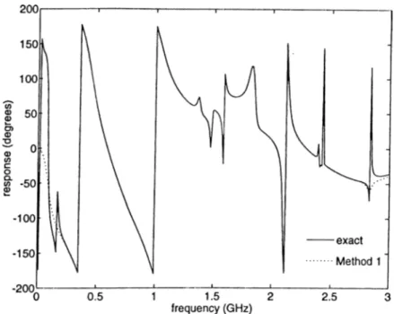
F igu re 4.2: Frequency response comparison .

The magnitude of load voltage is plotted in Fig. 4.2 with solid line as a function of frequency. We also find a 6th order Fade approximation for the load voltage,

1/ / _ 0-5000 - 0.05015 - 0.01465^ + 0.00185^ + 0.00025“^ - O.OOOO5® “ 1.0000 + 1.14975 + 0.345552 + 0.1253s3 + O.OIII5'' + 0.002455 _ 0.OOOO56

The approximated response is shown with dot-dashed line in F5g. 4.3.1. The dashed line in the same figure represents a 25th order Fade approximation. Since the exact response is periodic in frequency, it is impossible to approximate it with a rational polynomial function of finite degree even if the order of approximation is very high. However, this is not true for practical circuits which contain many energy storage lumped elements as well as lossy transmission lines. In such cases, the network functions are not periodic, i.e. they are rational functions of mixed polynomials and exponentials of 5, and, as 5 approaches to infinity their values become zero. This situation makes it possible to approximate the actual response with a rational polynomial function.