C om mun. Fac. Sci. U niv. A nk. Ser. A 1 M ath. Stat. Volum e 67, N umb er 2, Pages 50–63 (2018)
D O I: 10.1501/C om mua1_ 0000000861 ISSN 1303–5991
http://com munications.science.ankara.edu.tr/index.php?series= A 1
PORTFOLIO OPTIMIZATION UNDER PARAMETER UNCERTAINTY USING THE RISK AVERSION FORMULA
SIBEL ACIK KEMALOGLU, GULTAC EROGLU INAN, AND AYSEN APAYDIN
Abstract. The Markowitz portfolio optimization model has certain di¢ cul-ties in practise since real data are rarely certain. The robust optimization is a recently developed method that is used to overcome the uncertainty situ-ation. The technique has been recently suggested in the portfolio selection problems. In this study, two kinds of portfolio optimization problems are pre-sented: (i) the risk aversion portfolio optimization problem based on the clas-sical Markowitz framework, and (ii) the max-min counterpart problem based on the robust optimization framework. In the application, the two models are performed on a real-world data set obtained from BIST (Borsa Istanbul). Nu-merical results show that the ob jective function values of the classical solution and the robust solution are similar to each other. It can be said that the robust model, which works as well as the classical model in the uncertainty situations, can be used instead of the classical model and also that the optimal solution obtained in the uncertainty situation is robust to parameter perturbation.
1. INTRODUCTION
The main objective of the portfolio optimization problem is to choose the optimal portfolio with minimum variance from the set of all possible portfolios for any given level of expected return. Markowitz [22] formulated the …rst mathematical model for portfolio selection in the literature. After Markowitz, Sharpe [26] developed the Capital Asset Pricing Model (CAPM) and then Linter [19] and Mossin [24] used the Markowitz theory in their studies. In the literature, there are various other portfolio optimization methods developed in the context of the portfolio theory besides Markowitz, such as safety-…rst models, elliptical distributions, value at risk-based optimization, maximizing the performance measures EVA and RAROC and modelling the uncertainty of input parameters [10].
Received by the editors: August 15, 2016; Accepted: June 30, 2017. 2010 Mathematics Subject Classi…cation. 91B30, 91G10, 91B26.
Key words and phrases. Mean-Variance Optimization, Risk Aversion Formulation, Robust Optimization.
c 2 0 1 8 A n ka ra U n ive rsity C o m m u n ic a tio n s Fa c u lty o f S c ie n c e s U n ive rs ity o f A n ka ra -S e rie s A 1 M a t h e m a tic s a n d S t a tis tic s . C o m m u n ic a tio n s d e la Fa c u lté d e s S c ie n c e s d e l’U n ive rs ité d ’A n ka ra -S é rie s A 1 M a t h e m a tic s a n d S t a tis t ic s .
The Markowitz mean-variance portfolio optimization is a well-known investment theory that is widely used in allocating the assets. Its biggest in‡uence can be seen on the practice of portfolio management. The theory is focused on evaluating and managing the risks and returns of a portfolio of investments. This is highly advan-tageous as the resulting “optimized” portfolio will either have the same expected return with fewer risks than before or a higher expected return with the same level of risk. The Markowitz mean-variance optimization problem has several alterna-tive formulations that are used in practical applications. One of these alternaalterna-tive formulations is using a risk aversion coe¢ cient in the model, which is called the risk aversion formulation. This study handles the risk aversion formulation of the classical Markowitz model.
Although the Markowitz model is successful in the theory, there are various challenges of the model. The parameter uncertainty is an important issue in the optimization problems. In the Markowitz model, the uncertainty in the market parameters a¤ects the optimal solution of the problem. Thus, the results cannot be reliable enough. There are numerous studies in the literature to overcome the di¢ culties of the Markowitz model: Chopra and Ziemba [8] studied the estimated parameters. Broadie and Chopra [6] used the estimation errors in their study. Chopra [7] and Frost and Savarino [12, 13] presented a method related to the portfolio weights. Chopra et al. [9] used the James-Stein estimator for the means, Klein and Bawa [16], Frost and Savarino [12], and Black and Litterman [5] used the Bayesian estimation of means and covariances [19].
An underlying assumption of Markowitz’s model is that the precise estimates of i and ij have been obtained. Consequently, i and ij are treated as known
constants; however, asset returns are variable. It is reasonable to conclude that a model which treats returns as known constants will produce a portfolio whose realized return is di¤erent from the optimal portfolio return given by the objective function value. In particular, when the realized asset returns are less than the es-timates used to optimize the model, the realized portfolio return will be less than the optimal portfolio return given by the objective. Therefore, it is worthwhile ex-ploring the alternative frameworks, such as the robust optimization, for application to the portfolio selection problem. Although the distributions of asset returns are uncertain, in the robust optimization framework, it may be asserted that and , or both, belong to an uncertainty set, the bounds of which can be de…ned [15].
The aim of the method is to obtain a solution that is robust to the parameter uncertainty and estimation errors. In this framework, the robust counterpart of the original problem is handled. The robust problem is in fact the worst-case formulation of the original problem.
The …rst studies in the robust optimization framework are given in the studies of Ben-Tal and Nemirovski [2], [3], [4]. The …rst study handled the robust approach for linear programming. The other studies introduced the robust framework for convex programming. In these studies, it is assumed that the model parameters are
unknown, but they are bounded and belong to the speci…c uncertainty sets de…ned by historical knowledge. The aim of the robust (worst-case) approach is to obtain the optimal solution of the model which is robust to the parameter uncertainty and the worst-case situation. The robust counterpart of the original problem is handled in the robust model.
Goldfarb and Iyengar handled various robust portfolio selection problems in their study, such as the robust mean-variance portfolio selection, the robust mini-mum variance problem, the robust maximini-mum return problem, the robust maximini-mum Sharpe Ratio problem, and the robust value at risk problem [14].
There are many latest references in the literature about the robust portfolio selection problem. Wang and Cheng [28] considered the robust portfolio selection problem which has a data uncertainty described by the (p, w)-norm in the objective function. Balbás A., Balbás B. and Balbás R. [1] handled portfolio selection prob-lems under risk and ambiguity. Yu X. [29] developed a multi-period mean-variance model where the model parameters change according to a market with Markov random regime switching. Nalan G. and Canakoglu E. [25] considered a portfo-lio selection problem under temperature uncertainty. They introduced stochastic and robust portfolio optimization models using weather derivatives. Lot… S., Salahi M. and Mehrdoust F. [20] used the robust optimization approach to address the ambiguity in the conditional value-at-risk minimization model.
The aim of this study is to introduce the risk aversion portfolio selection prob-lem under the input parameter uncertainty. This problem is called the (maxmin) robust counterpart of the risk aversion problem. Moreover, it is aimed to obtain the optimal portfolio (the optimal solution of the robust problem) under this un-certainty and to compare the solution with the classical risk aversion solution.
In Inan [16] and Inan [17], the robust optimization approach is studied on the portfolio optimization problem. Numerical results showed that the classical optimal solution and the robust optimal solution gave similar values to the objective func-tion. As a result, the optimal solution obtained in the uncertainty case is robust to the uncertainty case. The …nding in the study is consistent with these studies.
The rest of this paper is organized as follows: In Section 2, the Markowitz port-folio optimization model and another alternative model, the risk aversion problem, is introduced. Section 3 presents the robust portfolio optimization method. The (max-min) robust counterpart of the problem is given. Finally, the max-min prob-lem is converted into the classical maximum probprob-lem by the Lagrange method. In Section 4, a numerical example of the model with a real data set is handled. The data is taken from BIST (Borsa Istanbul). In Section 5, some conclusions in certain and uncertain situations are given.
2. MARKOWITZ MEAN-VARIANCE PORTFOLIO OPTIMIZATION PROBLEM
Harry Markowitz published his study and formed the basis for the mean-variance optimization “Portfolio Selection” in 1952. He suggested that investors should create the optimal portfolio based on the balance between the expected return and the risk. In the Markowitz portfolio model, the returns are de…ned as the mean vector, and the risk is de…ned as the variance of return. The model uses the opti-mization and probability methods together under uncertainty. The model comprises the return matrix, the mean vector and variance-covariance matrix components.
Suppose that an investor has a portfolio comprised of n risky assets, denoted as Si The return of the security Si is de…ned as Ri, and the weight of the i:security
in the portfolio is de…ned as Xi.
The model can be created in two frameworks: (i) minimizing the risk of the portfolio for a certain level of expected return, (ii) maximizing the return of the portfolio for a certain level of risk.
The …rst model is given as,
min Xt X tX n X i=1 Xi = 1 Xi 0; i = 1; :::; n (2.1)
The second model is given as,
max tX Xt X n X i=1 Xi = 1 Xi 0; i = 1; :::; n (2.2)
where ; are constant, which are called the level degree. The descriptions of the model components are given as follows:
(Rk1; :::; Rkn)t represents the n kinds of returns at time k (k = 1; :::; m), where
Rki is the return of i:securities, i = 1; :::; n; k = 1; :::; m. The total data matrix is
represented as, 2 6 4 R11 ::: R1n .. . ... Rm1 ::: Rmn 3 7 5 (2.3)
The return vector is denoted as R = [R1:::Rn]tin m period, it contains the expected
value (mean) of each security. The expected vector of R is denoted as; = [ 1::: n]t
The input parameters and are not certain. It is very di¢ cult to estimate the correct values of these parameters. In the Markowitz model, the estimates of these parameters are used as follows:
= [ 1::: n]t (2.4) = Pmk=1Rk1 m ::: Pm k=1Rmkn t
and the covariance matrix is given by,
= 2 4 11 ::: 1N N 1 N N 3 5 (2.5)
Here; ijis the covariance between asset i and asset j.
The corresponding variance is given as,
ij2= m X k=1 (Rki i) Rkj j m 1 (2.6)
Thus, the random return vector R is represented by the ( ; ), [25].
There are two di¤erent de…nitions of R. One of them is the random vector. In …nance applications, one should use the adjusted (from splits and dividends) stock prices to make calculations. However, it is di¢ cult to obtain the adjusted stock prices from the splits and dividends, so only the closing prices are used in the study. The alternative model that combines the risk and the return of the objective function can be created using the coe¢ cient of risk aversion. The risk aversion formulation problem is de…ned as,
max 0X X0 X
X0l = 1; l = [1; 1; :::; 1] (2.7)
where, is the risk aversion coe¢ cient. When the investor is exposed to the uncer-tainty situation, the risk aversion coe¢ cient can be used to reduce that unceruncer-tainty. If is large, the aversion to the risk is high. For example, the risk-averse investor might make an investment in treasury bonds that have low but guaranteed expected returns. Otherwise, if is small, the aversion to the risk is low. For example, the risk-loving investor might make an investment in stocks, the options of which have high expected returns but also high risks.
3. ROBUST PORTFOLIO OPTIMIZATION PROBLEM
In spite of the theoretical success of the mean-variance model, practitioners have shied away from this model. The solution of optimization problems is often very sensitive to perturbations in the parameters of the problem. Since the estimates of the market parameters are subject to statistical errors, they are very sensitive to the perturbations in the inputs. The results of the optimization problems may not be very reliable. There are a number of discussions on how to decrease or eliminate the possibility of using incorrect inputs for the optimization problem. Various aspects of this phenomenon have been extensively studied in the literature on portfolio selection.
Michaud [23] proposed to use the technique of resampling. In his study, he suggested resampling the input parameters from a con…dence region and then aver-aging the cumulative portfolios that were obtained by each pair of sampling data. The main idea is that if resampling was performed enough times, the averaged op-timal portfolio would be more stable and less sensitive to the perturbations in the inputs. But when the amount of assets becomes large, this method is not useful and e¢ cient [21].
The robust optimization is the one of the aspects in the portfolio selection prob-lems [14]. In the robust approach, the worst-case formulation of the original optimization problem, called the robust counterpart of the problem, is handled. The robust counterpart of the classical risk aversion model is used in this study.
In [11], the (maxmin) robust counterpart of the risk aversion model is given as max X 2U (^)min 0 X X0 X X0l = 1; l = [1; 1; :::; 1] (3.1)
In the problem, it is assumed that the expected return vector is unknown but belongs
to the speci…c uncertainty set U (^). Many special uncertainty sets are de…ned for
the uncertain parameters in the literature. In this study, the uncertainty set for is taken as
U (^) = f =( ^)0( ) 1( ^ ) 2g (3.2)
where the parameters of the model are de…ned as follows: ^ :The estimated expected return vector
:The true expected return vector = 1
T ; Estimation error covariance matrix
T : Return data observations for N assets: : small number ( > 0)
The aim of the problem is to determine the weight vector X, which is robust to the uncertainty and the worst-case realization of the parameter.
For solving the robust (maxmin) problem easily, the problem is converted to the standard maximum optimization problem as follows:
Firstly, the uncertainty set is written as a constraint, then the problem can be written as
min 0X X0 X
( ^)0( ) 1( ^) 2 (3.3)
To solve this problem, the Lagrangian method can be used. The Lagrangian of the problem takes the form,
L ( ; ) = 0X X0 X 2 ( ^)0( ) 1( ) (3.4)
The optimal values of and are obtained by the …rst order condition as
= ^ 1 2 X (3.5) = 1 2 q X0 X (3.6)
Finally, by substituting the expressions in the Lagrangian form, the robust problem is obtained as max 0X X0 X q X0 X X0l = 1: (3.7) 4. APPLICATION
In this section, the robust portfolio selection approach, which was originally presented in the study by Fabozzi et al., is suggested. The data set is taken as the daily closing prices of nine securities that cycled in BIST 100 between 20.08.2013 and 20.08.2015. In the study, the daily stock price is chosen instead of the monthly stock price because the number of monthly stock price, which is 24 (for two years), may not be enough for the application.
The securities taken from the automotive sector belong to Balat, Asuzu, Daos, Karsn, Tmsn, Froto, Toaso, Ttrak, and Otkar. The returns of the securities were calculated according to the expression ln (Pt=Pt 1) of the closing prices. Here;
Pt: Closing prices of t: day
The average vector , the variance covariance matrix , and the estimation error covariance matrix M are calculated on the returns. Here;
M =
1 T T :Return data observations for N assets
In this study, T is given as 502 days between the designated dates (20.08.2013– 20.08.2015). The return vector , the variance covariance matrix and the
estimation error covariance matrix are obtained as follows. Note that the values in the variance covariance matrix are multiplied by 1000.
= 2 6 6 6 6 6 6 6 6 6 6 6 6 4 0:00000620 0:00157000 0:00088650 0:00018563 0:00063045 0:00069976 0:00043500 0:00091629 0:00054343 3 7 7 7 7 7 7 7 7 7 7 7 7 5 = 0:000623 0:000047 0:000363 0:000214 0:000249 0:000291 0:000283 0:000238 0:000200 0:000047 0:000804 0:000076 0:000024 0:000119 0:000047 0:000102 0:000053 0:000039 0:000363 0:000076 0:000869 0:000306 0:000324 0:000338 0:000340 0:000396 0:000213 0:000214 0:000024 0:000306 0:000429 0:000146 0:000216 0:000226 0:000281 0:000137 0:000249 0:000119 0:000324 0:000146 0:000607 0:000254 0:000297 0:000188 0:000158 0:000291 0:000047 0:000338 0:000216 0:000254 0:000674 0:000337 0:000243 0:000213 0:000283 0:000102 0:000340 0:000226 0:000297 0:000337 0:000765 0:000239 0:000177 0:000238 0:000053 0:000396 0:000281 0:000188 0:000243 0:000239 0:000598 0:000149 0:000200 0:000039 0:000213 0:000137 0:000158 0:000213 0:000177 0:000149 0:000378 = 0:001246 0:000093 0:000725 0:000429 0:000497 0:000582 0:000566 0:000476 0:000400 0:000093 0:001607 0:000152 0:000048 0:000239 0:000094 0:000204 0:000105 0:000077 0:000725 0:000152 0:001739 0:000611 0:000648 0:000676 0:000680 0:000791 0:000426 0:000429 0:000048 0:000611 0:000858 0:000293 0:000433 0:000451 0:000562 0:000275 0:000497 0:000239 0:000648 0:000293 0:001215 0:000507 0:000595 0:000376 0:000315 0:000582 0:000094 0:000676 0:000433 0:000507 0:001348 0:000675 0:000486 0:000426 0:000566 0:000204 0:000680 0:000451 0:000595 0:000675 0:001529 0:000479 0:000354 0:000476 0:000105 0:000791 0:000562 0:000376 0:000486 0:000479 0:001195 0:000298 0:000400 0:000077 0:000426 0:000275 0:000315 0:000426 0:000354 0:000298 0:000756 The classical model and the robust model, which have been de…ned in Section 2 and Section 3, are handled in the application. The models are given as follows:
The classical risk aversion portfolio optimization problem
max 0X X0 X
X0l = 1; l = [1; 1; :::; 1] The robust problem
max 0X X0 X
q X0
X X0l = 1
In the …rst case, the problem (2.7) is solved for the di¤erent 20 values of ,which is chosen by the information given in the Risk Aversion Formula by Fabozzi et al. [11]. The is chosen with an increase of 0.2. The [0,4] interval can be divided into smaller pieces so the number of can be increased.
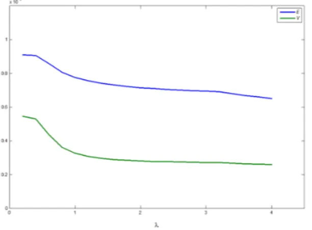
For the di¤erent values of , the movement of the expected return, the variance and the objective function value are seen in the related Figure 1, Figure 2 and Figure 3.The …gures show that when the value of increases (The aversion to risk is high–the risk-aversion investor), the values of the expected return, the variance and the objective function decrease. For the small values of (the aversion to risk
Figure 1. The movement of E : Expected V alue and V : V ariance for the classical problem
Figure 2. The movement of E and V for the robust problem
is low–the risk-lover investor), the values of the expected return, the variance and the objective function increase. In this case, it can be said that if the investor prefers the high expected return, the high risk must be considered.
In the robust case, when the expected return parameter is robust, the aim is to show the movement of the optimal solution to the parameter uncertainty. For this aim, the robust problem, which is given in (3.7), is solved for di¤erent and values.
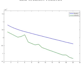
Figure 3. The movements of the objective functions for the classical problem and the robust problem
Table 1. The di¤erences between the objective function values for the classical and the robust problem
f_classical(x) f_robust(x) 0.2 0.0004380 0.4 0.0004408 0.6 0.0004546 0.8 0.0004869 1.0 0.0003630 1.2 0.0002022 1.4 0.0006047 1.6 0.0006361 1.8 0.0006652 2.0 0.0005666 2.2 0.0007187 2.4 0.0007442 2.6 0.0007688 2.8 0.0007929 3.0 0.0008167 3.2 0.0008400 3.4 0.0008634 3.6 0.0008103 3.8 0.0009110 4.0 0.0009252
If there is a need to compare the solution of the robust problem with the solution of the classical problem, it is observed that for the same values, the expected
return of the classical problem is larger than that of the robust problem. At the same time, its variance is smaller than the variance of the robust problem. In this situation, an investor should prefer the classical model.
On the other hand, the performances of portfolio models are measured by the Sharpe Ratio (SR) method. The Sharpe Ratio is de…ned as
SR = pE (rp) V ar (rp)
:
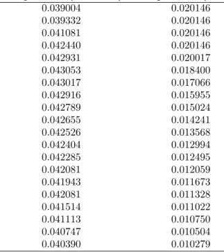
High SR values mean high performance. The Sharpe Ratio values obtained for the classical and the robust problem are presented in Table 2.
Table 2. The Sharpe ratio values for the classical and the robust problem. Sharpe ratio (Classical) Sharpe ratio (Robust)
0.039004 0.020146 0.039332 0.020146 0.041081 0.020146 0.042440 0.020146 0.042931 0.020017 0.043053 0.018400 0.043017 0.017066 0.042916 0.015955 0.042789 0.015024 0.042655 0.014241 0.042526 0.013568 0.042404 0.012994 0.042285 0.012495 0.042081 0.012059 0.041943 0.011673 0.042081 0.011328 0.041514 0.011022 0.041113 0.010750 0.040747 0.010504 0.040390 0.010279
It is seen that the classical Sharpe Ratio values are higher than the robust Sharpe Ratio values. Therefore, it can be said that the performance of the classical problem is better than the performance of the robust problem. However, in the uncertainty situations, it is recommended that the robust problem be used, which works as well as the classical problem.
5. CONCLUSION
The portfolio optimization model of Harry Markowitz can be created in two frameworks, which minimize the risk of the portfolio for a certain level of expected return and maximize the return of the portfolio for a certain level of risk. In spite
of the theoretical success of the mean-variance model, practitioners have avoided this model. The alternative model that combines the risk and the return of the objective function can be created using the coe¢ cient of risk aversion. The solution of optimization problems is often very sensitive to perturbations in the parameters of the problem. In the literature, there are many alternative methods suggested to overcome the parameter perturbations. The robust optimization is one of the most commonly used models in the uncertainty case.
The results show that when the value of increases, the values of the expected return, the variance and the objective function decrease. It means that the aversion to risk is high here, so it can be said that the investor is the risk-aversion investor. For the small values of , on the other hand, the values of the expected return, the variance and the objective function increase. Here, the aversion to risk is low, so it means that the investor is the risk-lover investor. In this case, it can be said that if the investor prefers the high expected return, the high risk must be taken into consideration.
If the solution of the robust problem is to be compared with the solution of the classical problem, it is observed that for the same values, the expected return of the classical problem is larger than the robust problem. At the same time, its variance is smaller than the robust problem variance. In this situation, an investor should prefer the classical model. The classical solution obtained in the certainty situation and the solution obtained in the uncertainty situation give similar values at the objective function. Consequently, it can be said that the optimal solution in the uncertainty situation is robust to ambiguity of the parameter . The robust model, which works as well as the classical model in the uncertainty situations, can be used instead of the classical model.
Finally, the performances of portfolio models are measured by the Sharpe Ratio (SR) method. It is seen that the classical Sharpe Ratio values are higher than the robust Sharpe ratio values; however, the robust problem, which works well to overcome uncertainty, should be preferred in the uncertainty situations.
In the future studies, the problem can be solved for di¤erent values of and . The data was taken from the automotive sector in this study. In order to improve the study, it is possible to investigate other sectors. In the modelling part, the short-selling is forbidden. However, in theory it is possible to allow short-selling. Hence, allowing the sort-selling will be studied in the future. The solutions can be compared for all these situations.
References
[1] Balbas, A., Balbas, B. and Balbas, R., Good deals and benchmarks in robust portfolio selection, European Journal of Operational Research, 250(2), (2016), 666-678.
[2] Ben-Tal, A. and Nemirovski, A., Robust convex optimization, Math. Oper. Res., 23(4), (1998), 769–805.
[3] Ben-Tal, A. and Nemirovski, A,. Robust solutions of uncertain linear program,. Oper. Res. Lett., 25(1), (1999), 1–13.
[4] Ben-Tal, A. and Nemirovski, A., Lectures on modern convex optimization, Society for Indus-trial and Applied Mathematics (SIAM), Philadelphia, PA, (2001).
[5] Black, F. and Litterman, R., Asset allocation: Combining investor views with market equi-librium, Technical report, Goldman, Sachs & Co., Fixed Income Research, (1990).
[6] Broadie, M., Computing e¢ cient frontiers using estimated parameters, Ann. Oper. Res., 45, (1993), 21–58.
[7] Chopra, V. K., Improving optimization,. J. Investing, (Fall), (1993), 51–59.
[8] Chopra, V. K. and Ziemba, W. T., The e¤ect of errors in means, variances and covariances on optimal portfolio choice, J. Portfolio Manag., (Winter), (1993), 6–11.
[9] Chopra, V. K., Hensel, C. R., and Turner, A. L., Massagin mean-variance inputs: Returns from alternative investment strategies in the 1980s, Manag. Sci., 39(7), (1993), 845–855. [10] Engels, M., Portfolio Optimization: beyond Markowitz, Master’s Thesis, Leiden University,
(2004).
[11] Fabozzi, F. J., Kolm, P. N., Pachamanova, D. A., & Focardi, S. M., Robust portfolio opti-mization and management, John Wiley & Sons, (2007).
[12] Frost, P. A. and Savarino, J. E., An empirical Bayes approach to e¢ cient portfolio selection, J. Fin. Quan. Anal., 21, (1986), 293–305.
[13] Frost, P. A. and Savarino, J. E., For better performance: constrain portfolio weights, J. Portfolio Manag., 15, (1988), 29–34.
[14] Goldfarb D., Iyengar G., Robust Portfolio Selection Problems, Mathematics of Operations Research, Vol. 28. No 1, (2003). 1–38.
[15] Gregory, C., Dowman, K.D. and Mitra, G., Robust Portfolio and Portfolio Selection: The cost of robustness, European Journal of Operation Research 212, (2011), 417–428.
[16] Inan Eroglu, G., Apayd¬n, A., Robust Optimization in Portfolio Analysis. Ph.D. Thesis, Ankara University, (2013).
[17] Inan Eroglu G., Apayd¬n A., Robust Quadratic Hedging Problem in Incomplete Market: For One Period and Exponential Asset Price Model, Selcuk Journal of Applied Mathematics Vol 16. No 2., (2015), pp. 13–26.
[18] Klein, R. W. and Bawa, V. S., The e¤ect of estimation risk on optimal portfolio choice, J. Finan. Econ., 3, (1976), 215–231.
[19] Lintner, J., Valuation of risky assets and the selection of risky investments in stock portfolios and capital budgets, Review of Economics and Statistics, 47, (1965), 13–37.
[20] Lot… S., Salahi M. and Mehrdoust, F., Robust portfolio selection with polyhedral ambiguous inputs, Journal of Mathematical Modelling,Vol. 5, No. 1, 2017, pp. 15–26.
[21] Lu, C-I., Robust Portfolio Optimization, Ph.D. Thesis, School of Mathematics, The Univer-sity of Birmingham,(2009).
[22] Markowitz, H. M., Portfolio Selection, The Journal of Finance. New York, (1952), 77–91. [23] Michaud R.O., E¢ cient Asset Management, Harvard Business School Press, Boston,(1998). [24] Mossin, J., Equilibrium in capital asset markets, Econometrica, 34(4), (1966), 768–783. [25] Nalan G., and Canakoglu, E., Robust portfolio selection problem under temperature
uncer-tainty, European Journal of Operational Research, 256 (2), (2017), pp. 500–523.
[26] Sharpe, W., Capital asset prices: A theory of market equilibrium under conditions of risk, Journal of Finance, 19(3), (1964), 425–442.
[27] Tanaka H., Peijun G and Turksen, B., Portfolio Selection Based on Fuzzy Probabilities and Possibility Distributions, Fuzzy sets and systems, 111.3, (2000), 387-397.
[28] Wang, L. and Cheng X., Robust Portfolio Selection under Norm Uncertainty, Journal of Inequalities and Applications, 2016: 1, (2016), 164.
[29] Yu, X., Regime dependent robust portfolio selection model, Journal of Interdisciplinary Mathematics. Vol 19: Issue 3, (2016), 517-525.
Current address : Sibel ACIK KEMALOGLU, Ankara University, Faculty of Sciences, Depart-ment of Statistics, Ankara,TURKEY
E-mail address : [email protected]
ORCID Address: http://orcid.org/0000-0003-0449-6966
Current address : Gultac EROGLU INAN, Ankara University, Faculty of Sciences, Department of Statistics, Ankara,TURKEY
E-mail address : [email protected](Corresponding Author) ORCID Address: http://orcid.org/0000-0002-3099-9949
Current address : Aysen APAYDIN, Ankara University, Faculty of Applied Sciences, Depart-ment of Insurance and Actuarial Science, Ankara,TURKEY
E-mail address : [email protected]