CELLULAR MANUFACTURING SYSTEM
DESIGN
a thesis
submitted to the department of industrial engineering
and the institute of engineering and science
of bilkent university
in partial fulfillment of the requirements
for the degree of
master of science
By
Hesna M¨uge Yayla
July, 2003
Assoc. Prof. Dr. M. Selim Akt¨urk (Supervisor)
I certify that I have read this thesis and that in my opinion it is fully adequate, in scope and in quality, as a thesis for the degree of Master of Science.
Prof. Dr. Erdal Erel
I certify that I have read this thesis and that in my opinion it is fully adequate, in scope and in quality, as a thesis for the degree of Master of Science.
Asst. Prof. Dr. Alper S¸en
Approved for the Institute of Engineering and Science:
Prof. Dr. Mehmet B. Baray
Director of the Institute Engineering and Science ii
SELECTION DECISION FOR CELLULAR
MANUFACTURING SYSTEM DESIGN
Hesna M¨uge Yayla M.S. in Industrial Engineering
Supervisor: Assoc. Prof. Dr. M. Selim Akt¨urk July, 2003
In today’s world, customers expect product variety. However, non-uniform products complicate the manufacturing processes significantly. In this study, we solved the cellular manufacturing system design and the technology selection problems simultaneously while taking the changing market dynamics into consid-eration. Cellular manufacturing system design problem aims the identification of existing part families and machine groups, while the technology selection decision determines the appropriate technology for the facility.
In order to integrate the market characteristics in our model, we proposed a new cost function. Further, we modified a well known similarity measure in order to handle the operational capability of available technology. This new coefficient is employed at the identification of part families. The technology selection deci-sion is based on the individual properties of parts, namely the production volume, variability of the demand, and the design stability of the part. Integration of the product variety at the design stage leads us to the use of flexible machining sys-tems and dedicated manufacturing syssys-tems at the same facility. In the thesis, our hybrid technology approach is presented via a multi-objective mathemati-cal model. A filtered-beam based lomathemati-cal search heuristic is proposed to solve the problem efficiently.
Keywords: Cellular manufacturing systems, technology selection, product variety.
H ¨
UCRESEL ¨
URET˙IM S˙ISTEMLER˙INDE ¨
UR ¨
UN
C
¸ ES¸˙ITL˙IL˙I ˘
G˙IN˙IN TEKNOLOJ˙I SEC
¸ ˙IM˙I KARARINA
ETK˙ILER˙I
Hesna M¨uge Yayla
End¨ustri M¨uhendisli˘gi, Y¨uksek Lisans Tez Y¨oneticisi: Do¸c. Dr. M. Selim Akt¨urk
Temmuz, 2003
G¨un¨um¨uz pazarlarında ¨ur¨un ¸ce¸sitlili˘ginin sunulması bir zorunluluk haline gelmi¸stir. Ancak ¨ur¨un ¸ce¸sitlili˘gi, ¨uretim a¸samasında bir¸cok zorlu˘gu da be-raberinde getirir. Bu ¸calı¸smada, de˘gi¸sen pazar gereklilikleri g¨oz ¨on¨une alınmı¸s ve h¨ucresel ¨uretim sistemleri tasarımı ile aynı anda teknoloji se¸cimi kararı da verilmi¸stir. H¨ucresel ¨uretim sistemleri tasarımı, sistem i¸cinde varolan par¸ca ailelerinin tanımlanması ve uygun makine gruplarının belirlenmesi esasına dayanır. Di˘ger yandan, teknoloji se¸cimi kararı da tasarımı yapılan tesiste kul-lanılacak teknolojiye karar verir.
Pazar ¨ozelliklerini modelimize katabilmek i¸cin yeni bir ama¸c fonksiyonu ¨onerilmi¸stir. Buna ek olarak, varolan makinelerin operasyonel yeteneklerinin modelde kullanılmasına olanak sa˘glamak amacıyla ¸cok bilinen bir benzerlik kat-sayısı yeniden d¨uzenlenmi¸stir. Benzerlik katsayıları par¸ca ailelerinin belirlen-mesinde kullanılmaktadır. Ayrıca, modelde teknoloji se¸cimi kararı, par¸caların bireysel ¨ozelliklerine dayandırılmı¸stır. ¨Ur¨un ¸ce¸sitlili˘ginin tasarım a¸samasında g¨oz ¨on¨une alınması, sonu¸cta esnek ve adanmı¸s teknolojilerin bir ¨uretim tesisinde aynı anda kullanılması gereklili˘gini ortaya ¸cıkarmı¸stır. Bu tezde, ¨onerilen melez teknoloji yakla¸sımı, ¸cok ama¸clı bir matematiksel modelle a¸cıklanmaktadır. Ayrıca, s¨oz konusu problemin olurlu ¸c¨oz¨um¨un¨un bulunabilmesi i¸cin filtrelenmi¸s ı¸sın yerel tarama y¨ontemine dayalı bir algoritma ¨onerilmi¸stir.
Anahtar s¨ozc¨ukler : H¨ucresel ¨uretim sistemleri, teknoloji secimi, ¨ur¨un ¸ce¸sitlili˘gi.
I would like to express my sincere gratitude to my supervisor Assoc. Prof. Dr. M. Selim Akt¨urk for his instructive comments in the supervision of this thesis. His encouragement, patience, understanding and great helps bring this thesis to an end.
I would like to express my special thanks and gratitude to Prof. Dr. Erdal Erel and Asst. Prof. Dr. Alper S¸en for showing keen interest to the subject matter and accepting to read and review the thesis.
I would like to thank to my good friends M. C¸ a˘grı G¨urb¨uz for his encourage-ment about the graduate study, and Ediz S¸aykol for his unlimited support at all stages of my study. I also would like to thank Ayten T¨urkcan, Banu Y¨uksel and Hakan G¨ultekin for their academic support and patience.
I also would like to thank my dear friends Halil S¸ekerci and Onur ¨Ozk¨ok for their unforgettable friendship and morale support during this two years time. I also would like to thank to my officemates, Evren Emek, Sibel Alumur, A˘gcag¨ul Yılmaz and ˙I. C¸ agatay Kepek for their friendship.
Finally, I dedicate this thesis to my lovely parents, M¨ukrime and Osman Nuri Yayla, and my dear husband A. Melih K¨ull¨u. Without their unlimited patience, support and encouragement, I could not have finished this study.
1 Introduction 1
2 Literature Review 4
2.1 Cellular Manufacturing Systems . . . 4
2.1.1 Machine Group - Part Family Identification Methods in Literature . . . 6
2.1.2 Assumption Domain and Model Characteristics . . . 7
2.1.3 Algorithms in Literature . . . 11
2.2 Technology Selection Literature . . . 18
2.3 Motivations of the Study . . . 21
3 Problem Statement 22 3.1 Problem Definition and Assumptions . . . 23
3.1.1 Basic Assumptions of The Model . . . 24
3.1.2 Basic Definitions Used in The Model . . . 25
3.1.3 Contributions . . . 26
3.2 Mathematical Model . . . 37
3.2.1 Parameters of the Model . . . 37
3.2.2 Decision Variables of the Model . . . 38
3.2.3 Objectives of The Model . . . 39
3.2.4 Constraints of The Model . . . 42
3.3 Summary . . . 45
4 Solution Approach 47 4.1 Outline of The Algorithm . . . 48
4.2 Stage I - Finding an Initial Solution . . . 49
4.3 Stage II - Local Search Heuristic . . . 57
4.4 Summary . . . 64 5 Experimental Design 66 5.1 Experimental Setting . . . 66 5.1.1 Factors A and B . . . 67 5.1.2 Factor C . . . 69 5.1.3 Factor D . . . 71 5.1.4 Factor E . . . 73
5.1.5 Parameters of The Experimental Design . . . 74
5.2 Experimental Results . . . 79
6 Conclusions and Future Work 90 6.1 Results . . . 91 6.2 Future Research Directions . . . 92
A Fuzzy Analysis Algorithm 103
B Initial Stage Results of Hybrid Algorithm 106
C Final Results of Hybrid Alg. with b=3 114
D Final Results of Hybrid Alg. with b=6 122
E Initial Stage Results of Dedicated Algorithm 129
F Final Results of Dedicated Alg. with b=3 137
G Final Results of Dedicated Alg. with b=6 145
H Global Minimum Objective Values 153
3.1 Traditional Product Life Cycle . . . 29 3.2 Possible Product Variety Cost Function Values . . . 32 5.1 Machine-Part Incidence Matrix . . . 75
3.1 Volume Costs in Product Variety Cost Function . . . 28
3.2 Demand Variation Costs in Product Variety Cost Function . . . . 30
3.3 Design Stability Costs in Product Variety Cost Function . . . 31
4.1 Problem Complicating Items . . . 48
5.1 Experimental Design Factors . . . 67
5.2 Factor A . . . 67
5.3 Factor B . . . 68
5.4 Average Demand Ratios . . . 68
5.5 Demand - Age Ratios . . . 70
5.6 Factor C . . . 71
5.7 An example PRM . . . 72
5.8 Factor D . . . 73
5.9 Factor E . . . 74
5.10 Machine Investment Costs . . . 76 x
5.11 Machining Center Specifications . . . 77
5.12 Improvements for Each Factor . . . 82
5.13 Dis-Similarity Objective (f1) . . . 83
5.14 Product Variety Cost Objective (f2) . . . 84
5.15 Throughput Time Objective (f3) . . . 85
5.16 Monetary Objective (f4) . . . 85
5.17 Intercellular Movement Objective (f5) . . . 86
5.18 Improvements for Selected Factor Combinations - I . . . 86
5.19 Improvements for Selected Factor Combinations - II . . . 87
Introduction
Business world of the 21stcentury witnesses an expanding global competition with increased variety of products and low demand. A company that wants to stay in this market should develop new manufacturing strategies. Old manufacturing technologies fail to meet the increasing demand for customized production.
In today’s world, market is no longer satisfied with uniform products. While the customers are expecting product variety, it makes the manufacturing processes considerably difficult. Known manufacturing systems become inadequate to per-form high variety production with low costs. Product variations in manufacturing brings high investment in equipment, high tooling costs, complex scheduling and loading, lengthy setup time and costs, excessive scrap, and high quality control costs.
Another effect of today’s competitive environment is the change in product life cycles. The manufacturer has not spacious time for product design and pro-duction plan. The new product should rapidly be introduced to the market. Moreover, the total lifetime of the product has significantly decreased. In such an environment, the manufacturer cannot invest in dedicated lines at the whole facility. Because, the product design is likely to change before the dedicated facility has been paid for. This has implications for integration of flexible manu-facturing systems. Flexible technology can be used both for existing designs and
for future re-designs of the products.
Around the world, batch manufacturing is the dominant manufacturing ac-tivity. In literature, it is said to account for 60 to 80 percent of all manufacturing activities. However, batch manufacturing industries cannot compete in today’s global market. Planning, controlling and scheduling must be simplified, ma-terial handling and setup times should be reduced, WIP inventories should be decreased, and quality must be improved. Furthermore, integration of design and manufacturing has to be achieved in order to provide customization to the market.
Group technology (GT) provides a gateway to achieve all these. Implementa-tion of GT in manufacturing environment is the Cellular Manufacturing System. Machines are grouped into cells to produce a group of parts having similar design attributes or manufacturing requirements.
In today’s world, technology selection is a more important issue. While design-ing a manufacturdesign-ing system, the designer has considerably many alternatives. Es-pecially flexible technology offers a variety of machines, some of which are highly capable in terms of operations. Today, there exist ‘Done in one’ machines, which may process a part in just one setup.
Cellular manufacturing system design (CMSD) problem is very complex in nature. It is being studied for the last three decades. However, today, grouping of parts and machine selection problems are even harder because of the strong competition and product variety encountered in the new millennium. In litera-ture, different approaches are proposed to solve CMSD problem. Methods used to identify machine-part families can be divided in three groups:
- Visual Inspection Method
- Part Characteristic Based Systems - Production Process Based Systems
part routings, machine clustering requirements, layout types, etc. However, as far as we know, no study exists which takes product life cycle and technology selection attributes into account while determining the part families and machine groups simultaneously. In Chapter 2, the existing approaches to solve the cell formation problem and technology selection literature are reviewed. The advantages and disadvantages of the existing literature are discussed.
In our study, we will analyze single product attributes leading to variety. Processing times and available machine capacities will be taken into consideration while identifying part families and machine groups. Furthermore, a technology selection scheme is proposed for machine group formation. The problem is stated with the underlying assumptions in Chapter 3. In the same chapter, a mixed integer programming model is proposed to solve the problem. The model has five minimization objective functions regarding dissimilarity in part families, product variety costs, throughput time, machine investment, maintenance and labor costs and finally intercellular movement. This multi-objective mathematical model has machine capacity, utilization and cell size constraints.
The proposed mathematical programming model cannot be solved in a rea-sonable computation time because of the numerous binary and integer variables and quadratic functions used in the model. Consequently, a local search heuristic is proposed to solve the problem. The proposed algorithm has two main stages. In the first stage of the algorithm, a known fuzzy analysis is implemented by using an adapted similarity measure. According to the results of this fuzzy analysis, initial part families and machine groups are identified by the algorithm. In the second stage, filtered beam search principles are employed to improve the initial solution.
The proposed algorithm is discussed in detail in Chapter 4. The efficiency of the algorithm is tested by a number of randomly generated problems. In Chapter 5, the experimental results are analyzed and the findings about the algorithm are summarized. In the last chapter, the discussion about the study and some future research directions are provided.
Literature Review
The cellular manufacturing and technology selection problems are studied sepa-rately in literature. That is, cellular manufacturing system models presume the technology is given and in most cases it is taken to be dedicated. Further, there exists no study incorporating market information to the CMSD problem. On the other hand, technology selection literature deals with a given partition of prod-ucts. However, in real life applications, the manufacturer should make technology selection and cell formation decisions simultaneously while taking the changing market dynamics into consideration.
In this chapter, we review the literature on cellular manufacturing systems, and technology selection. CMSD problem is discussed in §2.1, in §2.2 technology selection literature is briefly introduced, and in §2.3 the motivations of our study is provided.
2.1
Cellular Manufacturing Systems
The nature of production processes can be classified in three groups: intermittent, continuous and repetitive [67]. If the demand is occurring at intervals and the jobs are different from each other, production is said to be intermittent. It is
best to implement a standard machine layout, which is known as job shop layout. Nevertheless, the time part spends for waiting, travelling and setup is significantly high with such a layout. The time lost yields to low productivity.
On the other hand, if the production is in large scale and for a few part types, production has a continuous character. With such a layout, it is best to have the machines arranged in a sequence. This type of layout is known as flow shop layout. The cost of production is lowest in this case. However, to change the layout for production of a different part is a serious problem with such a layout. When the demand is repetitive, the best production system is the batch production. Around the world, batch manufacturing is the dominant manufacturing activity. It accounts for 60 to 80 percent of all manufacturing activities [66]. However, batch manufacturing industries cannot compete in today’s global market.
The concept of Group Technology (GT) has risen to reduce WIP inventories, setups, material handling distances, and batch sizes. It was originally introduced as a single-machine concept in Russia by Mitrofanov in 1966 [49]. It is further extended to be a manufacturing principle which identifies related or similar parts and processes to take the advantages of the similarities that exist during all stages of design and production.
GT has several significant benefits. Material handling time is minimal since the part is completely processed within the cell. Furthermore, since the cell con-sist of the required machines, parts move from one machine to other completing the production much faster. In CMS, throughput time depends on the operation with the maximum processing time, whereas in batch production systems, it de-pends on the total processing time of the whole part. Setup time is also reduced by the similar part groupings. The development in technology further contributes to the reduction in setup. Moreover, improvement in quality by the immediate feedback and increase in job satisfaction of labor forming teams in the cell are other benefits of the GT. The CMSD problem is therefore basically focused on the identification of appropriate family membership of parts and formation of machine groups accordingly.
2.1.1
Machine Group - Part Family Identification
Meth-ods in Literature
In this subsection, visual inspection method, part characteristic based systems, and production process based systems are discussed briefly.
2.1.1.1 Visual Inspection Method
This method is mainly based on experience. The inspector analyzes the parts, and according to their geometric similarities, families are determined [51]. Although Burbidge reports in 1971 that the method can be used to distinguish up to 2000 parts, today it is rarely used in practice [12].
2.1.1.2 Part Characteristic Based Systems
Part characteristic based systems are also known as part coding and classification analysis (PCA). PCA based methods group similar parts or separate dissimilar parts based on predetermined attributes. The code used to identify the part is a string of characters possessing information about the part. The PCA methods use parts coding schemes, which act as an instrument for the efficient recording, sorting, and retrieval of information [33].
There are three types of codes: Monocodes, Polycodes, and Mixed Codes. In literature, there exists various coding systems, e.g. BRISCH BIRN, CODE, MICLASS, OPITZ, KC-1. Extensive discussion on coding systems can be found in Hyer and Wemmerlov [33]. Generally coding schemes emphasized the identifi-cation of part families based on similarity in function, shape, etc. However, parts having similar shapes may have totally different manufacturing requirements. Hence, without any information about the machine groups, CMSD problem still has no clear answer.
2.1.1.3 Production Process Based Systems
Production oriented approaches solve part family formation problem based on the similarity in processing requirements of parts. These systems have the greatest amount of research attention. Most production oriented systems use routing of parts to determine the relationship between parts and the machines [51].
These approaches utilize either a simultaneous or sequential algorithms to define machine groups and part families. The sequential procedure determines the part families (or machine groups) first, followed by machine selection (or part allocation). The simultaneous procedure solves the machine group - part family formation problems concurrently [67].
2.1.2
Assumption Domain and Model Characteristics
Evaluation of design decisions can be categorized as relating to either system structure or system operation. During a design process, both structure and op-eration should be considered. In their review paper, Wemmerlov and Hyer [82] listed typical considerations related to system structure as equipment and tooling investment, equipment relocation cost, floor space requirements, manufacturing flexibility, extend to which parts are completed in the cell and existence of inter and intra movements of operators and material. The assumptions used to identify the problem characteristics might be either general or specific to each model. In literature, nine assumption domains are reported [51]:
1. Layout Type 2. Setup Time
3. Machine Clustering Requirements 4. Nature of Demand
6. Batch Size
7. Production Flow Policy
8. Number of machines per Machine type 9. Operation times
Few studies work on unknown demand. Harhalakis et al. [30] and Seifoddini [60] studied random product demand in cell formation problem. The authors mainly focused on the robustness over a certain range of demand variation ignor-ing any other market characteristic such as the age of the product or the number of design changes that the part underwent. Further, the authors use part-machine incidence matrix, assuming the only available technology is the dedicated tech-nology.
The model of Fine and Freund [21] provides a firm the flexibility to respond to future demand variations, but at the expense of the increased cost of investment. The authors perform a stochastic study on the system performance.
Many of the CMSD problem models assume the demand for each part is known, and constant over the planning horizon [51]. This assumption is far from reality. Part demand nature changes with part’s position in the life cycle. Prod-uct life cycle concept provides an appealing and readily understandable analysis for considering future growth opportunities and drawbacks. In contrary to the stability assumption, as time passes mean demand increases slowly at first and has high deviation at this introduction phase. At the growth phase, mean de-mand increases more quickly and deviation decreases. When the product is at maturity and saturation phases, it enjoys high and stable demand. Finally, de-mand decreases at the decline phase and before the dede-mand falls to zero, the product fades away from the market.
As far as we know, characteristics of the market has not been studied in the CMSD literature. Many parts have evolving designs to satisfy the changing demands of customers [76]. Without considering the age and the frequency of design changes of the part, researchers carried out their calculations.
To have more realistic models, researchers should incorporate the product life cycle concept instead of taking the demand constant and stable over time. Especially in 21st century, while the life cycles are getting shorter, designs are changing frequently and demand is subject to a significant decrease, constant demand assumption is no longer valid.
Arrangement of machines in a GT cell is generally assumed to be circular layout. Most of the models deal with the part family - machine group formation and do not consider actual manufacturing process activities such as scheduling and lot sizing. Setup times are also generally not included in the models.
When machine clusters are mutually separable, a machine can belong to one and only one cell. Some models assume machines could belong to more than one group. This may lead to a decrease in system efficiency by duplication. King et. al. and Kusiak et al. eliminate exceptional parts by subcontracting or forcing them to belong to one of the existing groups as discussed in [38] [41] and [42]. It is generally assumed that the model have m machines with one or more copies per machine type. The processing time of each machine for each operation on each part is also assumed to be known or varies probabilistically.
Based on these assumptions, in the literature models are built with the fol-lowing attributes:
• Decision variables represent actions or policy decisions concerning the
sys-tem:
– Number of machines of a given type to be assigned to a given cell – Number of parts or machines assigned to any given cell
– Number of operations or tool copies per part per group – Batch size
• Objectives: Several objectives of GT are cited in the literature. Ballakur
and Steudel list eight such objectives [8]: – Min intercellular travels
– Min intracellular travels
– Min setup time or Max machine scheduling flexibility – Max similarity (Min dissimilarity)
– Min total production cost
– Min exceptional element costs (subcontracting, duplication) – Min machine idle time
– Max machine utilization
• Constraints:
– Number of groups (cells or part families) – Number of parts per group
– Number of machines per group – Machine capacity
– Each part, machine or both belongs to one part family or machine group
– Annual operating budget
– Tool or processing requirement of parts
In their review paper, Shambu, Suresh and Pegels [65] provide a taxonomy that summarizes operational issues and impact of cellular manufacturing. The authors figured out that some issues remain unclear in the literature such as: consideration of product mix, demand rates, uncertainties, etc., investigation of the performance of the entire shop floor rather than a single machine or a single cell, and providing help to industry in making informed decisions on when to implement CM and to what extend.
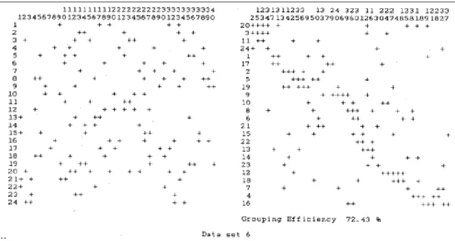
Wemmerlov and Hyer [83] stressed on the managerial aspects of cellular man-ufacturing applications. The authors raised questions on the operations strategy and social aspects of cellular manufacturing systems. Grouping efficiency is de-fined as the evaluative measure of the machine-part groups in cellular manufac-turing systems. The measures are reported both descriptively and quantitatively.
Sarker and Khan [57] presented a comparison of existing grouping efficiency mea-sures and proposed a new weighted grouping efficiency measure.
2.1.3
Algorithms in Literature
In this subsection, array based algorithms, similarity coefficient based clustering, mathematical programming, graph theoretic, and other approaches are discussed briefly.
2.1.3.1 Array Based Algorithms
CMSD solution identifies part families and machine groups for a production facil-ity. Each part family processed within a machine group with minimum interaction with other groups. In literature, the processing requirements of parts on machines is obtained from the routing cards. This information is represented in a matrix called the part-machine incidence matrix with 0 or 1 entries. A 1 in row i and column m shows that part i requires machine m for an operation.
This kind of representation has serious drawbacks. If a part requires more than one operation on a machine, this cannot be identified in the part machine matrix using a 0-1 representation. On the other hand, with the available tech-nology, there are flexible machines which can handle several operations with the same setup. A 0-1 matrix cannot represent any information about the flexible technology. In today’s world, an analyst should not disregard the flexible technol-ogy. In literature, there are several matrix manipulation algorithms [67]. After rearranging rows and columns of the matrix, part families and machine groups are identified:
BEA - Bond Energy Algorithm: McCormick, Schweitzer and White devel-oped BEA to identify natural groups that exist in complex data arrays [48]. This is a quadratic assignment based cluster analytic model. The authors
define the bond strength between any two adjacent elements in a machine-part incidence matrix as their product, and the bond energy as the sum of the bond strengths. The objective is therefore to maximize the bond en-ergy of the 0-1 matrix, resulting in a block diagonal matrix. It is reported that the final ordering is dependent on the initial row or column selected to initiate the process.
ROC - Rank Order Clustering: King [36] and [37] developed the ROC algo-rithm, which is the better known of the array-based clustering algorithms. Each row (column) in the part-machine matrix is read as a binary word. The procedure converts these binary words for each row (column) into dec-imal equivalents. The algorithm successively rearranges the rows (columns) in order of descending values until there is no change. However, even in well structured matrices it is not certain ROC will identify the block diagonal structure, and it possess computational difficulties.
ROC 2: King and Nakornchai [38] extended the basic ROC model to improve its computational efficiency. The new algorithm simultaneously sorts sev-eral rows and columns, thus enabling it to solve problems of much larger dimensions.
MODROC - Modified ROC: Chandrasekaran and Rajagapolan [15] identi-fied the fact that ROC has a tendency to collect all the 1’s in the top left corner. By removing this block of columns from the matrix and perform-ing ROC again, MODROC collects another set of 1s in the top left corner. This process will identify mutually exclusive part families but may contain overlapping machines.
DCA - Direct Clustering Algorithm: Chan and Milner [14] proposed the DCA, which rearranges the rows with the left-most positive cells (i.e. 1s) to the top and the columns with the top-most positive cells to the left of the matrix. Wemmerlov [81] provided a correction to the original algorithm to get consistent results. This procedure, again, may not necessarily always produce diagonal solutions, even if one exists.
present cluster identification and cost analysis algorithms to solve the machine-part grouping problem. In CIA, the machine-part incidence matrix is transformed into machine-part clusters using a form of cutting algorithm. It is not designed to decompose a matrix to a near-block diagonal form, but simply to identify disconnected blocks if there are any.
Modified CIA: In CIA, each element of the matrix is scanned twice. Boctor [11] proposed a new method where each element of the matrix is scanned only once.
2.1.3.2 Similarity Coefficient Based Clustering
Clustering is a mathematical method that is used to identify similar objects in a set. It is also used in the context of part-machine grouping. The methods of cluster analysis follow a set of steps [55]:
• Collect a data matrix, columns and rows of which stand for objects and
attributes (parts and machines).
• Using the data matrix, compute the values of a resemblance matrix
coeffi-cient to measure the similarity.
• Use a clustering technique to process the values of the resemblance
coeffi-cient.
Although the basic steps are constant, there is a wide range in the definition of the resemblance matrix and the choice of clustering method. The similarity and distance measures using binary part-machine incidence matrix have the same disadvantages of not possessing part specific information like the array-based methods. Similarity coefficient concept is first introduced by McAuley [47]. The proposed similarity coefficient is also known as the Jaccard’s similarity coefficient and it is widely accepted and used in the literature.
Seifoddini and Djassemi [61] modified Jaccard’s coefficient by adding produc-tion volume data. Tam [74] integrated the operaproduc-tion sequence informaproduc-tion in
the calculation of the similarity coefficient. Nair and Narendran [50] proposed a weighted machine sequence similarity coefficient to cluster machines. Gupta and Seifoddini [27] presented a similarity coefficient using production volume, routing sequence and unit operation time. Akturk and Balkose [2] solved the part-machine grouping problem using a multi-objective cluster analysis. The au-thors suggested a new dissimilarity measure based on design and manufacturing attributes and operation sequences.
Recently, Yin and Yasuda [84] proposed a new similarity coefficient to cope with cell formation problems that consider alternative process routings, operation sequences, operation times and production volumes of parts simultaneously.
In two articles Shafer and Rogers [63], [64] reviewed the different similarity and distance measures used in cellular manufacturing. Manufacturing features other than the information provided in the part-machine matrix such as part volume, part sequence, tool requirements, setup features, etc. can be considered while computing the similarity measure. Some of the known clustering algorithms in literature are as follows:
SLC - Single Linkage Clustering: McAuley [47] is the first to apply single linkage clustering to cluster machines. The data matrix to be cluster-analyzed is the part-machine incidence matrix. A similarity coefficient is first defined between two machines in terms of number of parts that visit each machine. Once the similarity coefficients have been determined for ma-chine pairs, SLC algorithm evaluates the similarity between two mama-chine groups.
CLC - Complete Linkage Clustering: The algorithm remains the same with SLC except at the step of similar machine choice. It combines two clusters at minimum similarity level rather than at maximum level as in SLC. ALC - Average Linkage Clustering: SLC and CLC are clustering based on
extreme values. Instead, it may be of interest to cluster by considering the average of all links within a cluster. SLC produces compacted trees; CLC extended trees; and ALC trees are intermediate between these extremes.
Seifoddini [59] presented a comparative study of the two similarity coeffi-cient based algorithms: SLC and ALC. The authors found that although SLC was relatively easy to apply, it might cause the chaining problem and produce more exceptional parts. ALC overcomes these drawbacks at a cost of more computation time.
LCC - Linear Cell Clustering: Wei and Kern proposed LCC [79], [80]. It clusters machines based on the use of a commonality score which defines the similarity between two machines. However, the worst case computational complexity of the algorithm is not linear as the name suggests.
2.1.3.3 Mathematical Programming and Graph Theoretic
Ap-proaches
The algorithmic procedures mentioned up to this point are heuristics. In litera-ture, there also exist mathematical models which can provide optimal solutions. The heuristics are also utilized as a starting point towards an optimal solution.
One of the first approaches to forming part families using mathematical pro-gramming was by Kusiak [40]. The objective of p-median model is to find f part families optimally, such that the distance between parts in each family is mini-mized with respect to the median of the family. The drawback of the model is that it only identifies part families. Srinivasan, Narendran and Mahadevan [72] proposed an assignment model for the part families and machine grouping prob-lem. The authors provided a sequential procedure to identify machine groups followed by identification of part families.
Selvan and Balasubramanian [62] present an integer programming formulation for grouping components based on their operation sequences. The objective of the model is to minimize the sum of material handling and machine idle costs subject to each component belonging to only one group, the one that minimizes the objective.
Some authors in literature integrate the production planning problem into cel-lular manufacturing systems. Akturk and Wilson [5] proposes a hierarchical cell loading approach to the hierarchical production planning problem simplified with CM shop configuration. Song and Hitomi [71] integrated production planning and layout decisions in CMSD problem at the same time. The authors define the flex-ibility as the optimal integration of production planning and cellular layout in a cellular manufacturing system. Schaller, Erenguc and Vakharia [58] proposed a mathematical approach for integrating the cell design and production planning decisions.
Choobineh [17] adopts a modified Jaccard similarity measure that uses op-erations sequences and proposes an integer programming formulation approach. Gunasingh and Lashkari [25], [26] propose two 0-1 integer programming formu-lations based on tooling requirements of the components (parts) in each family, available tooling on the machines, and processing times. Vakharia, Askin and Sen [75] present a 0-1 integer programming formulation with the objective of mini-mizing the total cost of machines required and intercell material handling costs, subject to each part being completely processed in each cell, machines required per cell, and number of cells visited by each part. Kandiller [34] used utiliza-tion levels, workload balances, exceputiliza-tional elements and intercellular densities to compare the efficiency of some well known cell formation methods.
The clustering algorithms and p-median model minimize the distance of parts to the family median. Nevertheless, the parts within a family interact with each other. Kusiak, Vanelli and Kumar [44] proposed a quadratic programming model for this purpose. Kusiak and Chow [43] represented the machine-part incidence matrix as a graph formulation. The authors showed three types of graph depend-ing on the representation of nodes and edges: bipartite graph, transition graph or boundary graph. Dahel and Smith [18] constructed a 0-1 integer programming formulation to design flexibility into cellular manufacturing systems. The flexibil-ity concept the authors indicate in their paper is the intercell routing flexibilflexibil-ity. This kind of flexibility reduces the proportion of parts being fully processed in one cell. Askin, Selim and Vakharia [7] studied demand flexibility simultaneously with routing flexibility.
Akturk and Turkcan [4] proposed a integer programming model to solve CMSD and layout problems simultaneously using a holonistic approach to maxi-mize profit of individual cells. The authors also considered operation sequences, alternative routings, production volumes and processing times in their study. A more detailed discussion about mathematical formulations and graph theoretical approaches can be found in Offodile et al. [51] and Singh [67].
2.1.3.4 Other Approaches
Utilization of mathematical formulations brought the chance to integrate more information on the CMSD problem such as part volume, processing times, oper-ation sequences, available machine capacity, etc. However, since the scope of the problem is broad, most of the proposed models cannot be solved optimally in a reasonable computation time.
On the other hand, the heuristics presented in former sections, although yield-ing an approximate solution in a reasonable computation time, are sensitive to the initial solution and groupability of the part-machine matrix. Hence, novel methods have emerged recently: Simulated annealing, genetic algorithms, neural networks, tabu search and beam search [67].
Simulated Annealing (SA) is inspired from the physical sciences. The design of SA is based on three key concepts [23]: The temperature controls the probability that a cost increasing solution will be accepted (in a min prob-lem). The equilibrium point concept determines the point where no further improvement is expected in the objective with additional sampling. The
an-nealing schedule defines the set of temperatures to be used and how many
interchanges to consider before reducing the temperature. Adil, Rajamani and Strong have implemented SA to the grouping problem [1].
Tabu Search (TS) is in many ways similar to SA [53]: they both move from one schedule to another with the next solution being possibly worse than the one before. The basic difference between TS and SA is the mechanism
used for approving a candidate schedule. In TS, at any stage of the process, a tabu list of mutations, which the procedure is not allowed to perform, is kept. For more information on tabu search see Glover [24].
Genetic Algorithms (GA): Holland developed GA as a random search tech-nique in 1992 [31]. It was originally inspired by an analogy with the process of natural evolution. The design of GA is based on six key concepts:
repre-sentation, initialization, evaluation function, reproduction, crossover, and mutation [28].
Neural Networks models mimic the way biological brain neurons generate in-telligent decisions. Biological brains are superior at problems involving massive amount of uncertain data. Thus, neural network models are po-tential tools to solve the cell formation problems.
Beam Search: Enumerative branch and bound methods are currently the most widely used methods for obtaining optimal solutions to NP-hard problems. Beam search is a derivation of the branch and bound algorithm [53]. It eliminates some of the branches in an intelligent way. The number of nodes reserved for further evaluation is the beam width of the search. For these nodes, a simple evaluation procedure is applied, and some more non-promising nodes are fathomed. The number of nodes selected for a thorough evaluation is the filter width. After the final evaluation, a set of promising nodes are selected for next iteration. The size of this set is equal to the beam width. Ow and Morton [52] provide a thorough analysis of a filtered beam search methodology for different scheduling problems.
2.2
Technology Selection Literature
Increased product variety, low unit costs and lead times, high levels of product quality are necessary conditions to survive in today’s markets. Large number of product variety, customized and instable product designs, increased interna-tional competition, the need to reduce manufacturing lead time, all require the
development of manufacturing technologies [66]. The development of computer integrated manufacturing systems addresses some of these problems. Neverthe-less, flexible manufacturing systems have high investment costs increasing the unit manufacturing costs. On the other hand, there still exists parts that have a standardized design and high production volume.
In literature, there are number of studies that analyze the trade off between flexible technology and dedicated technology. Singhal et al. [68] define the bene-fits of flexible technologies as the ability to respond quickly to changes in design and demand, lower direct manufacturing costs, improved quality, economies of scope, flexibility in scheduling. Basnet and Mize [10] provide a critical review on scheduling and control of flexible manufacturing systems. Sambasivarao and Deshmukh [56] classify and review the issues regarding the selection and imple-mentation of advanced manufacturing technologies.
Flexibility is the key concept used in the design of modern automated man-ufacturing systems. Every manman-ufacturing system is flexible to a certain degree. Barad and Nof [9] review CIM flexibility measures and provides a framework for analysis and applicability assessment. Gupta and Goyal [29] provide a com-prehensive review of the literature on flexibility. Since there are various types of factors that affect the system performance, there exists various types of flexibility:
• Machine Flexibility • Routing Flexibility • Process Flexibility • Product Flexibility • Production Flexibility • Expansion Flexibility • Volume Flexibility • Operation Flexibility
Flexible Manufacturing Systems (FMS’s) provide most of the above flexi-bilities to a facility. FMS’s also provide the ability to rapidly introduce new products to the market. This accelerates the implementation of flexible technol-ogy. Hutchinson and Holland [32] compared dedicated and flexible technologies. The authors simulated the effects of technology selection on manufacturing per-formance. Flexible technology is more preferable as the rate of new product introduction increases and as the average volume per part decreases. Fine and Li [22] studied optimality of automated manufacturing at some stages of the product and process life cycles. Li and Tirupati [46] constructed a mathematical program for selecting the optimal mix of dedicated and flexible technologies and timing of capacity additions to satisfy the deterministic demand over a finite planning horizon. Burstein [13]provided a convex programming model which incorporates production and technology selection decisions.
Some authors in the literature implement the multidimensional aspect of flex-ibility. Falkner and Benhajla [20] suggest to use the multi-attribute decision methods. Stam and Kuula [73] and Kuula and Stam [45] utilized multiple crite-ria optimization for FMS selection decisions. On the other hand, productivity, quality and flexibility are critical measures of manufacturing performance for jus-tifying the investment in computer integrated manufacturing systems. Son and Park [69], [70] study the economic measure of these three critical performance measures in advanced manufacturing systems.
There exist studies which considered technology selection problem simulta-neously with the facility location and capacity acquisition problems. Detailed information on this subject can be found in Verter and Dincer [78], Verter and Dasci [77], and Dasci and Verter [19]. Rajagopalan [54] and Li and Tirupati [46] studied technology selection problem integrated in the capacity expansion decision models.
Recently, Krishnan and Bhattacharya [39] studied the problem of technology selection and commitment under uncertainty. The authors formulate a mathe-matical model to compare a proven technology versus a prospective technology. The analysis shows the appropriateness of the different flexible design approaches.
2.3
Motivations of the Study
It is evident from the previous sections that the cellular manufacturing and tech-nology selection problems are studied separately in literature. That is, cellular manufacturing system models presume the technology is given and in most cases it is taken to be dedicated. Further, there exists no study incorporating market information to the CMSD problem. On the other hand, technology selection liter-ature deals with a given partition of products. However, in real life applications, the manufacturer should make technology selection and cell formation decisions simultaneously while taking the changing market dynamics into consideration.
PCA based methods use design similarity between part without consider-ing the manufacturconsider-ing requirements. Array based methods employ binary part-machine incidence matrices which possess no information about production vol-ume, design stability, or operation sequences. Heuristics and mathematical for-mulations are best suited to CMSD problem. Important criteria, such as pro-duction volume, processing times, load-unload times, machine investment and maintenance costs, available machine capacities can be handled simultaneously.
In general, it is assumed that the market is stable with highly standardized products with high and stable demand patterns. However, in 21st century, this is an unrealistic assumption. The market is no longer stable. Designs are evolving, production volumes are decreasing and life cycles are getting shorter. Thus, in order to design an efficient manufacturing system, analysts should incorporate this information effectively in the models.
In this study, our aim is to consider all important manufacturing system de-sign factors such as properties of market and available technologies. Further, the model that we constructed takes important manufacturing issues such as produc-tion volume, throughput times, utilizaproduc-tion levels, machine investment, mainte-nance and labor costs into consideration while identification of part families and machine groups is accomplished. In the following chapter, the problem is de-fined with the underlying assumptions and a mathematical programming model is proposed.
Problem Statement
Cellular manufacturing system design (CMSD) is primarily concerned with the formation of part families and machine groups leading to appropriate
manufac-turing cells in order to achieve the benefits of group technology. In literature,
various CMSD algorithms are proposed. In Chapter 2, these approaches to solve the problem are reviewed and it is emphasized that none of these procedures has taken market information and selection of available technology into consideration. In literature, it is generally assumed that the market is stable with highly standardized products with high and stable demand patterns. However, in 21st century, this is an unrealistic assumption. The market is no longer stable. Designs are evolving, production volumes are decreasing and life cycles are getting shorter. Thus, in order to design an efficient manufacturing system, we propose a new model to incorporate this information effectively.
Technology selection problem deals with selecting the best alternative among available technologies while designing a manufacturing system. Since the prod-uct life cycles have been shortening in today’s market, prodprod-uctivity, flexibility, service time, quality and reliability as well as costs have become the major con-siderations for survival in the market. Thus, firms should adopt the automated manufacturing technologies in order to keep their competitiveness. In our study, we provide a model that make use of the automated technologies while keeping
the dedicated technologies as an alternative.
In this study, an integrated approach is proposed to solve the cell design and technology selection problems simultaneously during the design of an advanced manufacturing system. We proposed a new cost function to integrate the mar-ket characteristics in our model. Further, we modified a well known similarity measure in order to handle the operational capability of available technology.
In section §3.1, the problem definition and our contributions to the definition are presented. In §3.2, a mathematical model is proposed to form manufacturing cells utilizing appropriate technology for management of product variety. In the last section §3.3, we present the concluding remarks about the problem.
3.1
Problem Definition and Assumptions
The aim is to solve the cellular manufacturing design problem and the technol-ogy selection problem simultaneously which, in general, is the case in real life problems. In today’s world, a firm should benefit from the available computer integrated technology while sustaining the use of economies of scale inherited in dedicated manufacturing.
In this multi-objective study, a modification of a well known similarity measure is utilized in order to form part families, and the technology selection decision is based on the individual properties of parts, namely the production volume, variability of the demand, and the design stability of the part. The market information is quantified via a newly introduced cost function in the model.
First, basic assumptions of the model are presented. In the second subsection, some definitions related to the model are given, in the third subsection new cost function and new similarity coefficient are introduced, and finally the model is presented.
3.1.1
Basic Assumptions of The Model
- There are N parts with different demand variabilities, design patterns and production volumes.
- There are O operations required for the processing of the parts that can be handled by some of the F M flexible machine types, or DM dedicated machine types.
- Available technologies are flexible manufacturing systems, and dedicated machines.
- Each machine can perform a number of operations which are known a priori. - The operations required in production of each part are known. Operation
sequences of the parts are not taken into consideration in this model. - Annual demand, age of the part, and the number of design changes up
to date are known a priori. These attributes play an important role in calculation of the new product variety cost function and determination of the appropriate technology.
- The processing time of each operation of each part on each machine is pre-determined. Processing times of parts are important not only because they are utilized in determining the number of machines required of each type, but also because they form a basis for the technology decision via deter-mining the throughput times. The processing times of flexible machines are longer compared to that of dedicated machines. In terms of only the processing times, dedicated technology is preferable.
- Load and unload times are assumed to be equal for each part-machine pair and known a priori, but on the average load/unload times for flexible machines are taken to be longer than that of dedicated machines. However, each part should be loaded and unloaded on a dedicated machine for one operation while the flexible machines can handle a number of operations with a single load/unload. The load-unload times are utilized for calculation of the throughput times together with the processing times and provides
a trade off to decide whether to process all the operations on a flexible machine or to process each operation on separate dedicated machines. - The machine investment, maintenance, and labor costs are assumed to be
known. They form a monetary basis for the decisions.
Under these assumptions, the following decisions need to be made:
- Part families
- Machine groups with appropriate technology - Part assignments to cells
- Operation assignments of each part to machines - Number of each machine type in each cell
3.1.2
Basic Definitions Used in The Model
Machine Capability Matrix (MCM)
It is a 0 − 1 matrix presenting the operational capabilities of the machines. Rows of MCM are reserved for the machine types, where columns are reserved for operation types.
MCM = MCM11 MCM12 . . . MCM21 MCM22 . . . ... ... . .. MCMmo =
1 if machine type m can perform operation o 0 otherwise
MCM has two basic blocks. Upper rows represent the values of dedicated machines. Thus, this block forms a unit matrix. Each row has only one
positive value, since each dedicated machine is defined by a specific opera-tion. Lower rows represent the values of flexible machines. In these rows, we observe more number of 1’s. As the number of 1’s in a machine’s row increases, we say the machine gets more flexible, since the machine flexibil-ity can be measured by the number of operations that can be handled by that machine. A representative MCM looks like the following:
MCM = 1 0 0 . . . 0 1 0 . . . 0 0 1 . . . ... ... ... ... 1 1 0 . . . 0 1 1 . . . 1 0 1 . . . ... ... ... ...
Part Requirement Matrix (PRM)
It is a 0-1 matrix presenting the processing requirements of the parts. Rows of P RM are reserved for the parts, where columns are reserved for operation types, as it is in the MCM . PRM = P RM11 P RM12 . . . P RM21 P RM22 . . . ... ... . .. P RMio =
1 if part i requires operation o 0 otherwise
3.1.3
Contributions
In order to integrate the market characteristics in our model, we proposed a new cost function. This is the first study to assign costs for design instabilities and
demand variations. We minimize these costs resulting from the offered variety in today’s markets.
Further, we modified a well known similarity measure in order to handle the operational capability of available technology. During the design of a cellular manufacturing system, it is generally treated that the only available technology is the dedicated technology. However, computer integrated manufacturing tech-nologies are provided for the use of manufacturers. In order to make use of this computer numerically controlled machines, we propose a new similarity measure during the design of cellular manufacturing systems.
3.1.3.1 Product Variety Cost Function
By the term product variety, we imply the fluctuations in three characteristics of a product in a production environment:
. Production Volume . Demand Pattern . Design Stability
Following notation associated with the product variety costs is used in the thesis:
cid : cost of assigning part i to a dedicated cell
cif : cost of assigning part i to the flexible cell
avol : production volume coefficient of the part
aσ : demand variation coefficient of the part
ades : design stability coefficient of the part
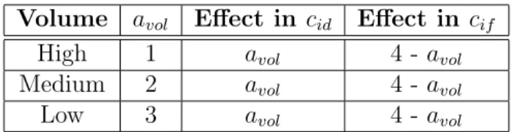
Production volume of a part can differ from part to part. A part can have a high production volume whereas another, but operationally similar part can have a very small production volume. If these two parts are assigned in the same
Volume avol Effect in cid Effect in cif
High 1 avol 4 - avol
Medium 2 avol 4 - avol
Low 3 avol 4 - avol
Table 3.1: Volume Costs in Product Variety Cost Function
cell, the frequent and interrupting set-up requirements can become a burden con-tradicting that set-up should have been an advantage of cellular manufacturing. To eliminate such a set-up problem, we should assign low-volume parts to FMS cell, whereas the high-volume parts to the cells composed of dedicated machines, namely dedicated cells.
We propose a costing scheme in Table 3.1 which is based on the volume characteristics of the parts. If the part is a low volume part, cost of assigning this part to a dedicated cell is 3, if it is a medium volume part, cost is 2, and for a high volume part, cost is only 1. Cost order is reversed for a flexible cell, which is 1 for low volume parts in flexible cells, 2 for medium volume parts, and 3 for high volume parts processed in a flexible cell. As a result of this volume cost, low volume parts tend to be processed in flexible cells, and high volume parts tend to be processed in dedicated cells.
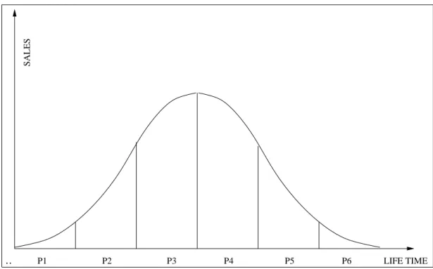
Demand pattern of the part is a more important attribute of the part. Even we can determine the expected demand for the part, we should also care about the variation of this value. The traditional product life cycle curve is provided in Figure 3.1. It is true that in the early stages of the typical life cycle (introduction phase), variations in demand are high. However, the demand has much less variation during the periods of its half life-time (saturation phase). If the life of a part is divided in 6 equal periods, deviation is high in period 1, medium in period 2 and 5, and low in period 3 and 4. Generally, at the end of fifth period, the production of the part is ceased. Thus, it is not wrong to assume that there exists no product of period 6.
.. P1 P2 P3 P4 P5 P6 LIFE TIME
SALES
Figure 3.1: Traditional Product Life Cycle
Ages of parts differ, resulting various demand patterns at the production floor. Suppose a part is in its half-time periods of life, and another part is newly introduced in the market. While the first part is enjoying a stable demand pattern, the second one is subject to peaks and digressions. It is known for the first part how much to be produced pretty surely, whereas the demand for second part can change at any time. It may increase or diminish by time. Thus, under a risk of fading, to allocate resources for the second part may not end up with satisfactory results. To deal with this situation, we should benefit from the flexibility of flexible manufacturing cells, and put an influence on the high-variation parts to be assigned to FMS cells.
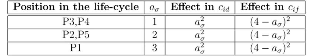
The proposed costing scheme is given in Table 3.2. The importance of the variation cost is emphasized by assigning the square power of the coefficients as the cost values. The coefficients are based on the life cycle positions of the parts. If the part is in its half life time periods, namely the 3rdand 4thperiods, coefficient is 1 and cost of assigning this part to a dedicated cell is only 1, if it is a newly
Position in the life-cycle aσ Effect in cid Effect in cif P3,P4 1 a2 σ (4 − aσ)2 P2,P5 2 a2 σ (4 − aσ)2 P1 3 a2 σ (4 − aσ)2
Table 3.2: Demand Variation Costs in Product Variety Cost Function introduced part, i.e in its 1st life period, the coefficient becomes 3 and cost gets as high as 9. On the other hand, a part which is in its 2nd and 5th life periods, is still subject to a variation in demand not as high as a newly introduced part, but not as small as a saturated part. It has a coefficient in the middle region, and cost is calculated to be 4.
Cost order is reversed for a flexible cell, which is 9 for saturated parts, 4 for medium volume parts, and 1 for newly introduced parts to be processed in a flexible cell. As a result of this costing scheme, parts that have high variations in demand tend to be processed in flexible cells, and parts that have stable demand patterns tend to be processed in dedicated cells.
Design stability is the most important attribute of the part. In today’s markets, more customized designs need to be made in order to catch up with the competition. Many parts have evolving designs to satisfy the changing demands of customers. However, some parts still have stable design patterns.
When a design is said to be stable, the operations required are exactly defined for the part. When it is evolving, new operations may be added or some may be discarded from the routing. Thus, to design a dedicated manufacturing cell for an evolving part is a total jeopardy. We should assign an evolving part to a dedicated cell if and only if we have no other alternative.
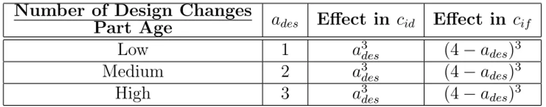
The proposed cost structure is provided in Table 3.3. The significance and superiority of the design stability is emphasized by assigning the triple power of the coefficients as the cost values. The coefficients are based on the average number of design changes per life time unit of the product. If the part has underwent a high number of design changes in relatively short amount of time,
Number of Design Changes
Part Age ades Effect in cid Effect in cif
Low 1 a3 des (4 − ades)3 Medium 2 a3 des (4 − ades)3 High 3 a3 des (4 − ades)3 Table 3.3: Design Stability Costs in Product Variety Cost Function average becomes high and coefficient is 3. Associated cost value of assigning this unstable part to a dedicated cell is calculated to be as high as 27. At the other end, if the part has a very stable design, i.e. average number of changes is low, coefficient becomes 1 and cost of processing this stable part in a dedicated cell is as low as 1. Similarly, a part with medium range number of design changes has a coefficient in the middle region, and cost is calculated to be 8.
Cost order is reversed for a flexible cell, which is 1 for unstable parts, 8 for medium volume parts, and 27 for parts having stable design patterns to be processed in a flexible cell. As a result of this costing scheme, parts that have unstable design patterns tend to be processed in flexible cells, and parts that have stable designs tend to be processed in dedicated cells.
After identification of the values of coefficients and associated cost values of parts, final product variety cost function values are calculated. Having assigned different weights to the attributes, we make use of the simplicity and power of additivity in our proposed cost function.
cid = avol + a2σ + a3des
cif = (4 − avol) + (4 − aσ)2 + (4 − ades)3
cid and cif are complementary costs. The more we prefer to assign a part to the flexible cell, the less we prefer to assign that part to a dedicated cell, and vice versa. The cost function have several important missions to be used in the solution procedure. It is basically used as a surrogate objective function of the model. Further, it provides us a strong basis for the selection of technology for each cell.
.. 0 1 2
1 2 3 4 5 6 7 8 9 10 11 12 13 14 15 16 17 18 19 20 21 22 23 24 25 26 27 28 29 30 31 32 33 34 35 36 37 38 39 40 Cost Function Values
O c c u re n c e
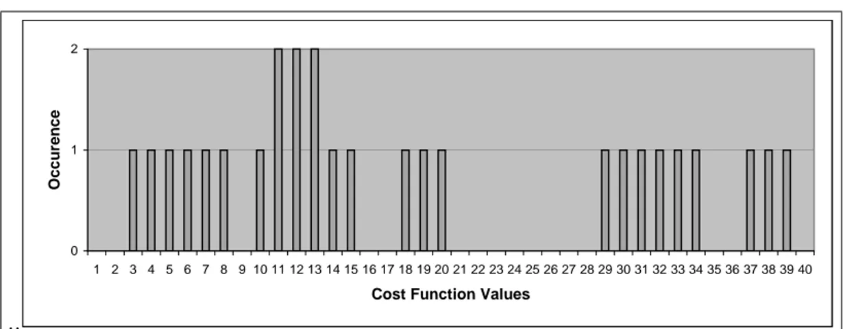
Figure 3.2: Possible Product Variety Cost Function Values
The range of the new cost function values begins from 3 and goes up to 39. All the possible observations of the cost function are calculated and plotted on the histogram presented in Figure 3.2. The same graph is true for both function values, cid and cif.
The observed values provide us very important information. Let the graph is plotted by the values of cid costs. The parts providing the lowest costs are most probable members of families being processed on dedicated cells, and the ones with highest costs are selected for being processed on flexible cells. However, when it comes to choose from the middle region of the values, the analyst cannot decide for a threshold value clearly. It is observed that there exists a big jump at level 20. However, as it can be seen on the graph, some values occur more than once. When the number of occurrences is taken into consideration, the smaller jump on the value 15 is more meaningful to represent a threshold value to choose between dedicated and flexible technology. This value is utilized at two very critical points in the algorithm, which are discussed in detail in the next chapter.
3.1.3.2 Modified Jaccard Similarity Coefficient
The first similarity coefficient defined in the literature was between two machines in terms of the number of parts that visit each machine. The resulting image is
a two-by-two matrix, where four types of matches are possible:
1 0
1 a b
0 c d
In this matrix, a is the number of parts visiting both machines, b is the number of parts visiting only the first machine, c is that of second machine, and
d is the number of parts not visiting any of the two machines. Jaccard coefficient
(JC) is the most often used coefficient in the similarity context. It is not only a powerful coefficient but also very simple and effective as follows:
JCmn =
a
a + b + c 0 ≤ JCmn≤ 1
JCmn shows the similarity between two machines, m and n, by calculating the ratio of common parts, to the total number of parts processed on these two machines. The main assumptions lying under this coefficient is that a specific operation can be handled by a specific machine, and whenever a part requires that operation, it has to visit that machine. However, with the available technology, an operation can be handled by several different types of machines. Thus, the assumption on which the coefficient is based has changed in today’s world.
With the change of one-to-one assignment of machine operation pairs, simi-larity context should also be adapted to the technological advancements. As a first step for this adaptation, as we cannot relate a part to a machine directly, we should utilize operations as an indicator of similarity.
Operational similarity can be applied in part-similarity context, where pre-viously a indicates the number of machines that both parts have operation and Jaccard is calculated as the similarity between parts i and j (JCij). With the new definition (JC0
ij), we may adapt a0 just as the number of common operations in both parts’ routings, b0 as the number of operations required only by part one, and c0 as that of part two.
JC0 ij = a0 a0+ b0 + c0 0 ≤ JC 0 ij ≤ 1
Even after this adaptation, Jaccard still has imperfections. In this new for-mulation, we still do not have the machine flexibility information. When this information is integrated in the coefficient, then the modification can be accom-plished fully.
The proposed model solves the calculation of similarity coefficient problem in two stages. A representative example is provided after the presentation of formal steps of the coefficient. In the first stage, a hypothetical manufacturing cell is designed to produce only the two parts. This cell is forced to have the minimum size without any other considerations, since we specifically need the numbers. As a second stage, we calculate the coefficient.
1. Design of a hypothetical manufacturing cell to find the minimum number of machines required to produce two parts in the same cell.
2. After the cell design, the following similarity table is formed between the two parts:
1 0
1 k l
0 m n
In this matrix, k is the number of machines where both parts have an operation, l represents the number of machines which are required only by first part, and m is that of second part. Then the Modified Jaccard Similarity Coefficient (MJCij) follows:
MJCij =
k
As we have found the minimum possible cell size in the first stage, we have also found the greatest possible k, the number of common machines in the same cell. Hence, the greatest the modified similarity between the parts, the more number of machines in common between the parts, leading to a part family produced in a manufacturing cell composed of the common machines.
In the solution procedure, we minimize the dissimilarity between the parts, and attain homogeneity among the part families. Since we use dissimilarity co-efficients in the model, a further calculation is needed. The Jaccard coefficient is defined from 0 to 1, and related dissimilarity is the complement of the coefficient value. Same range and complementarity applies to Modified Jaccard. Thus, the Dissimilarity Coefficient (DMJij) is:
DMJij = (1 − MJCij) 0 ≤ DM Jij ≤ 1
Example Let the available Machine Capability Matrix (MCM) and Part
Require-ment Matrix values of parts i and j are as follows:
MCM op1 op2 op3
m1 1 0 0
m2 0 1 0
m3 0 0 1
fm1 0 1 1
PRM op1 op2 op3
i 1 0 1
j 1 1 0
Jaccard coefficient finds the number of common operations between parts from the PRM and calculates the similarity as follows:
JCij =
op1
op1 + op2 + op3 =
1 3
On the other hand, The Modified Jaccard make use of the available flexible technology and calculates the coefficient as follows:
Step 1: Construction of a hypothetical cell to produce only parts i and j. In the minimum best possible cell configuration, we have machines m1 and fm1.