A polyhedral approach to quadratic assignment problem

ІД Г Р τ η П П АГіЙ ізТіГ·

B i ± f i

^ rrt-T'r·^ С*'*С»

¿ и в ш т т ш > 'ÏÔ Т Ш S S y U -I M B l'I - ÖF

a

NIGIXSBSI

í

^IG

V

AND THS IHSTİTUTS OF SÍ-

í

GHSSS

l

IHO İŞOD ТС

і

НЙСЗ

OF BXLKENT иш ѵггчоіт'т

:

n pa h tia l f u l f il l m e n t l f

тн Е'ЗіЕоин ст«а^:то

FOR THE DEGSHE OF

_OHTER OF SCIENCE

CíÁ -'■' ^ K

6

S

l â s i é

-*A. A . ;^:f| ^ '/ j?· . І / ( •O v ji; V ' 'ώ vj V w ' oJ· - .'· V J t ^

A POLYHEDRAL APPROACH TO QUADRATIC

ASSIGNMENT PROBLEM

A THESIS

SUBMITTED TO THE DEPARTMENT OF INDUSTRIAL

ENGINEERING

AND THE INSTITUTE OF ENGINEERING AND

SCIENCES

OF BILKENT UNIVERSITY

IN PARTIAL FULFILLMENT OF THE REQUIREMENTS

FOR THE DEGREEOF

MASTER OF SCIENCE

By

Ahmet Sertaç Murat Koksaldı

September, 1994

T.U

<9>A

t|02

Ill

I certify that I have read this thesis and that in my opin­ ion it is fully adequate, in scope and in^uality, as a thesis for the degree of Master c Science./

J

fa Akgül(Principal Advisor)

I certify that I have read this thesis and that in my opin­ ion it is fully adequate, in scope and in quality, as a thesis for the degree of Master of Science.

Assoc. Prof.

I certify that I have read this thesis and that in my opin­ ion it is fully adequate, in scope and in quality, as a thesis for the degree of Master of Science.

n

a

Assoc. Prop Omer Benli

Approved for the Institute of Engineering and Science:

ABSTRACT

A POLYHEDRAL APPROACH TO

QUADRATIC ASSIGNMENT PROBLEM

Ahmet Sertaç Murat Koksaldı

M.S. in Industrial Engineering

Supervisor: Assoc. Prof. Mustafa Akgiil

September, 1994

In this thesis, Quadratic Assignment Problem is considered. Since Quadratic Assignment Problem is JVP-bard, no polynomial time exact solution method exists. Proving optimality o f solutions to Quadratic Assignment Problems has been limited to instances of small dimension. In this study, Quadratic Assign­ ment Problem is handled from a polyhedral point of view. A graph theoretic formulation of the problem is presented. Later, Quadratic Assignment Poly­ tope is defined and subsets of valid equalities and inequalities for Quadratic Assignment Polytope is given. Finally, results of the experiments with a poly­ hedral cutting plane algorithm using the new formulation is also presented.

K e y w o r d s : Quadratic Assignment Problem, Quadratic Assignment Polytope, polyhedral cutting plane algorithm

ÖZET

KARESEL ATAMA PROBLEMİNE

POLYHEDRAL BİR YAKLAŞIM

Ahmet Sertaç Murat Koksaldı

Endüstri Mühendisliği, Yüksek Lisans

Tez Yöneticisi : Doç, Mustafa Akgül

Eylül, 1994

Bu tez çalışmasında, Karesel Atama Problemi ele alınmıştır. Karesel Atama Problemi

YP-zorlukta olduğu için, polinom zamanlı bir çözüm yöntemi mevcut değildir.

Olabilir çözümlerin en iyiliğinin ispatı ancak küçük boyutlu problemlerde mümkündür. Çalışmamızda, Karesel Atama Problemi polyhedral bir açıdan ele alınmıştır.

Karesel Atama Probleminin graf teorik bir ifadesi tanımlanmıştır. Daha sonra,

Karesel Atama Poytopu ve, geçerli ba^ı eşitsizlik ve eşitlik alt kümeleri tanımlanmıştır. Son olarak da, Karesel Atama Probleminin yeni ifadesinin kullanıldığı bir poly­

hedral kesen düzlem yöntemi ile yapılan testlerin sonuçları verilmiştir.

A n a h ta r S ö zcü k le r: Karesel Atama Problemi, Karesel Atama Poytopu, polyhedral kesen düzlem yöntemi

To my family and people who added value to my life

4

ACKNOWLEDGMENT

I would like to thank my advisor Mustafa Akgiil who has suggested such aji interesting topic for this study. I would also like to thank Assoc. Prof. Osman Oğuz and Assoc. Prof. Omer Benli for accepting to read and review this thesis. I would like to extend my thanks to my parents, my sister Ebru and my love Emine for their support and encouragement.

I greatly appreciate Levent Kandiller, Iradj Ouveysi and Fatih Yılmaz for their valuable remarks, guidance and encouragement.

Contents

1 I N T R O D U C T I O N 1

2 LITERATURE REVIEW

4

2.1 Mathematical Programming Formulations of Q A P ... 5

2.1.1 Nonlinear Integer Programming Form ulation... 5

2.1.2 Integer Programming F orm u lation s... 6

2.1.3 Mixed-Integer Programming F orm u la tion s... 7

2.2 Computational C om plexity... 9

2.3 Lower Bounds for Q A P ... 9

2.4 Exact Solution M e t h o d s ... 12

2.5 Heuristics ... 13

2.6 Probabilistic Asymptotic Behavior of Q A P ... 17

3 Q U A D R A T I C A S S I G N M E N T P O L Y T O P E 18 3.1 D efinitions... 19

3.2 General Methodology of Polyhedral Combinatorics ... 20

3.3 Graphical Representation and a New Formulation of QAP . . . 23 viii

CONTENTS I X

3.4 Partition and Layer Equalities for ... 26 3.5 Special Structures in G = {V, E )... 27 3.6 Branch and Cut Experim entation... 36

3.7 Leaf Equalities for QA'^ 39

List of Figures

3.1 Graph G for n = 3 ... 25

3.2 A t r ia n g le ... 28

3.3 Chordless cycle of length 7 ... 29

3.4 Chordless cycle of length m ... 33

List of Tabl(:3

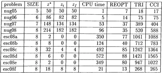
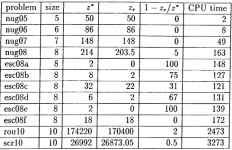
3.1 Branch and Cut E xperim en tation ...38 3.2 Results of Final hnear programming R e la x a t io n ... 41

Chapter 1

Introduction

Koopmans and Beckmann [40] are the first to state Quadratic Assignment Problem (Q A P ). While dealing with the allocation of plants to locations they realized that “The assumption that the benefit from an economic activity at some location does not depend on the uses of other locations is quite inadequate to the complexities of locational decisions.” This conclusion is the result of ex­ perimentation with the linear assignment models of location theory. Therefore they attempted to incorporate the cost of transportation between plants to the model. With the motivation of considering the interactions between plants, they introduced the QAP:

They consider n plants and n locations. Given

Cij : gross revenue obtained by assigning plant i to location j

a,fc : required commodity flow between plants i and k bji : unit transportation cost between locations j and /

Given n X n real matrices

A,

B and C , let Sn he the set of permutations over W where A/" = {1 ,2 ,..., n } and <y? G Sn· Then QAP is

z = min

^ 2

X / ~

^ 2

гe^íke^í ıe^í,,,

According to Koopmans and Beckmann, “ QAP seems to be close to the core 1

CHAPTER 1. INTRODUCTION

of location theory.”

Following Koopmans and Beckmann, many real life problems are stated as QAP:

In the wiring problem of Steinberg [68], n modules have to be placed on a board and be connected by wires. Given

aik : distance between positions i and k

bji : number of connections between modules j and / the aim is to minimize the total wire length.

Design of control panels and typewriter keyboards is another problem modeled as a QAP ( Burkard and Offermann [13], Pollatschek, Gershoni and Radday [59] ). Given

aik : the mean frequency of a pair of letters i and k in language L

bji : the time needed to press key / after pressing key j

their aim is to arrange the keys of a typewriter on the keyboard such that the time needed to write a certain text in language L is minimized.

For other fields of application see Burkard [9].

There is a strong interest in the exact solution algorithms for QAP. Since QAP is AiV- hard, no polynomial time algorithm is known. Existing exact solution algorithms, branch and bound, and cutting plane algorithms, are so ineffective that they can solve problems up to size n < 17 where as explicit enumeration can solve problems of size < 10.

We will handle the QAP from the polyhedral point of view. In the late 70’ies a new method. Polyhedral Cutting Plane Method, is introduced for combina­ torial optimization problems. Its roots lie in the seminal paper of Dantzig, Fulkerson and Johnson [19]. The idea is to define the feasible set of the combi­ natorial problem by linear inequalities and equalities, and algorithmically add those to the linear programming relaxation. Since it is impossible to know all the linear inequalities and equalities defining the underlying polytope, one works with a subset of facets. After solving the linear programming relaxation, violated facets are identified and added to the linear programming relaxation. One resorts to branching if no violated inequalities are found. This is what branch and cut is, use of cutting planes and branching sequentially until finding

CHAPTER 1. INTRODUCTION

the optimal solution.

In chapter 2 we will give a summary of solution methods, lower bounds, heuris­ tics and complexity results regarding QAP. Chapter 3 will be devoted to our studies. We mainly concentrate on symmetric problems, i.e. A and B are symmetric matrices. This is not merely a restriction because any QAP instance can be transformed to a symmetric QAP ( SQAP ) instance by the technique of Hadley, Rendl and Wolkowicz [34]. A graph theoretic formulation of QAP will be presented. Later quadratic assignment polytope will be defined and sets of valid equalities and inequalities for quadratic assignment polytope will be given. Results of a polyhedral cutting plane algorithm will also be presented. Chapter 4 consists of the discussion of our study and further areas of research.

Chapter 2

Literature Review

Koopmans-Beckmann formulation of the first chapter is a special type of Q A R Lawler [43] stated general QAP as:

Problem 2.1 (QAP)

Given

n“*

cost coefficients Cijki where i , j , k j

€

Af and AT =

{1,2,... , n},

let Sn be the set o f permutations over Af and (p

G

Sn-

Then QAP is

^ ~ X / X / "h X^ ^«.¥>(0

içAi

In Koopmans-Beckmann formulation cost coefficients c,jjt/ equal to aik-bp. Re­ searchers concentrated on Koopmans-Beckmann problems rather than general QAPs. Although some of the works are applicable to general QAPs, it is at least customary to use Koopmans-Beckmann type test problems. Burkard, Karish and Rendl [12] collected QAP instances used in the literature. All of these instances are Koopmans-Beckmainn problems.

2 .1

M a th e m a tic a l P ro g ra m m in g F orm u lation s

o f Q A P

Like other combinatorial problems QAP can be formulated as a mathematical programming problem. Mainly there are three classes of formulations:

1 . ) Nonlinear Integer Programming formulations, 2 . ) Integer Programming formulations,

3 . ) Mixed-Integer Programming formulations.

CHAPTER 2. LITERATURE REVIEW 5

2.1.1 Nonlinear Integer Programming Formulation

This formulation immediately follows from the problem statement. A permu­ tation of the set Af can be uniquely represented by a vector x G 7^"^ such that

X — (2:11, Xj2) *··> ·*·> ) ^n2î ··’^nn) where

1 if ip{i) = j V i J e A f Xij = , .

U otherwise

and XijS obey the following assignment ( multiple choice) constraints

Defining Assignment Polytope A P " to be:

A P ” = { .T € : X satisfies equations 2 and 3 }

Henceforth, QAP can be reformulated as:

P r o b le m 2.2

..?Vpn

_{E E E E}

kl

“f·

(1) — 1 I^jV Vj e Af ₍₂₎ a,’tj = 1 j€A/· Vi e Af ₍₃₎

CHAPTER 2. LITERATURE REVIEW

Since it is usually more difficult to deal with nonlinearities many researchers, in the hope of tractability, try to linearize the objective function. Next sections are devoted to these works.

2.1.2

Integer Programming Formulations

The first linearization technique was proposed by Lawler [43]. It simply replaces each quadratic term ,i.e XijXkh by a new binary variable yijki through imposing some constraints and transforms problem 2.2 to

P r o b le m 2.3 ^ie^í'^je^í^ke^íY^ıe^í^ijkiVijki A dijXij s.t. J

₂

jeAi^keJ\i^içAiyijki — -X%j T Xkl ^Vijkl ^ X e AP'^ yijki € {0) 1} V i,j,k ,i e M

T h e o r e m 2.1 (L aw ler) The feasible solutions of problems 2.2 and 2.3 can be placed in one-to-one correspondence with equal values of the objective functions. A feasible solution x of problem 2.2 corresponds to a feasible solution {x',y') of problem 2.3 if and only ifx = x'.

p r o o f:

Let X describe a feasible solution of problem 2.2. By letting = Xij Xkt,

all constrains of problem 2.3 is satisfied and both problems yield the same objective function value.

Conversely, let ( x', y') be a feasible solution of problem 2.3. Letting = 1 in a given solution, from assignment constraints

Xi, = 0 V; S M\ f i i ) (4)

Then, yijki = 0 unless j = ip(i) and / = It follows that

X] X]

y'ijkl -

1

CHAPTER 2. LITERATURE REVIEW

and this inequality is strict unless = 1. Now summing over all i, k

we have

,2

XI XI ( X]

y'ijkl )

^

unless y'ijf

.1

= 1 whenever x'- = x'f.^ = !.□

n

(6)

Lawler’s formulation has n'* additional binary variables and n“* + 1 additional constraints. Hence, this linearization besides giving some insight does not make the world easy. If you try to solve a problem of size, say 10, you will fed into }'our integer programming solver a problem with 10100 binary variables and 10021 constraints which is hopeless. This frustrating result caused researchers to look for smaller sized, more tractable linearizations.

2.1.3

Mixed-Integer Programming Formulations

As a remedy to the coiiiputational burden of introducing binary variables, continuous variables are used in linearization. Bazaara and Sherali [7] used ad­ ditional |n^(n — 1)^ continuous variables and 2n^ additional linear constraints. Frieze and Yadegar [25] proposed a method which uses the same number of continuous variables as Bazaara and Sherali [7] but introduces only con­ straints. Kaufman and Broeckx’s [39] linearization, which utilizes the method of Glover [29], is applicable only in the case of nonnegative objective function coefficients. It introduces new continuous variables and additional linear constraints. Another linearization technique which is of the same effectiveness, in terms of additional variables and constraints, is suggested by Oral and Ket- tani [48] [49]. Their method is applicable to general QAPs. We will discuss their method and further reduction techniques they employed for decreasing the number of binary variables. Defining a lower bound and an upper bound, respectively D~j and on the terms

A v <

E

E

s

A Î (7)

CHAPTER 2. LITERATURE REVIEW

P r o b le m 2.4

min E.-6ArEj6A^( A j ^ij + )

^ij ^ ^ijkl^kl ~ ~ Hfj ( 1 ~ Xij ) V i ,j G Af X e A P ’^

> 0

T h e o r e m 2.2 (O ral and K e tta n i) problem 2.2 is equivalent to problem 2-4 in the sense that they have the same optimal solution.

P r o o f:

Observe that each is subject to two constraints:

if Xij = 0 then iij > X ) dijkiXki - Dfj and (f,j > 0 ₍₈₎

if ^ij ~

1

then ^ij ^ ^ ^ ^ ^ dijkix/ii ^ij keAiteJ^

Given the definitions of Zl“ and Dfj, which imply that

and (ij > 0

₍₉₎

X X dijkiXki - Dfj

< 0

(10)

X X

dijkiXki — D - >

0

keAiieJ^

(11)

the constraints on reduce to:

>

0 if Xij = 0

EiteA/" EieA/" ^ij i^ ^ij — f

(12)

Since (f,j appears in the objective function as a linear term with a coefficient + 1, there could never be an optimal solution to problem 2.4 in which is greater than the minimum possible value. Thus the requirements on in problem 2.4 can just as well be written

io =

0 if Xij = 0

Ylk€^í ^ijkl^kt Dij if Xij — 1

(13)

Substituting for ^ij in the objective function of problem 2.4 we get the original problem. □

CHAPTER 2. LITERATURE REVIEW

Thus Oral and Kettani [48] [49] introduces new continuous variables and additional constraints to linearize QAP. This is the smallest and most general linearization as of today. Bounds D~j and D^j can be computed simply by the method of Kaufman and Broeckx [39]:

^ 0 max„ I^ EdijkiXki

(14)

(15)

keA/lÇAi

Both are simple Linear Assignment Problems.

They further reduce the number of binary variables at the cost of additional constraints. They managed to reduce the number of binary variables from to nlog2 « while adding n{n + 2) constraints. This reduction enables the use of mixed integer programming codes for moderate sized problems.

2.2

C o m p u ta tio n a l C o m p le x ity

It is known that traveling salesman problem is a special case of Koopmans- Beckmann problem where one of the matrices A or B is a permutation matrix [9]. Therefore QAPs are M V- hard. Sahni and Gonzales [65] showed that QAPs belong even to the hard core of this complexity class. That is, they proved that even the full approximation problem is AiV - complete: Let an arbitrarily small e be given, for all problem instances find a permutation Tp

with objective function value z{îp) such that z* - z{i^)

< e (16)

2.3

Low er B o u n d s for Q A P

Since QAP is A/”'P-complete implicit enumeration methods are mostly used as exact solution techniques. Especially these are special branch-and-bound

CHAPTER 2. LITERATURE REVIEW ₁₀

methods. Good lower bounds (LBs) increase the effectiveness of branch-and- bound procedures. Therefore a great amount of work is done on finding good LBs.

The first LB proposed is due to Gilmore [28] and Lawler [43] independently. Computation of Gilrnore-Lawler (GL) bound is cis follows:

Given problem 2.1, compute for each pair i , j 6 Ai,

6ij = rnin _{>:,k'p(k) (17)}

e,j is a lower bound on the cost of interactions between assignment i ^ j

and remaining assignments. In computing Cij, only the pairwise interactions between assignment i j and the remaining assignments is considered. If we let fij = Cjj + fij represents a LB on the assignment of i to j. fi/s

form an nxn matrix. Then,

2 > GL = min fim (18)

is a LB on problem 2.1. e,j’s can be computed by solving a Linear Assignment Problem of size n — 1. We have to compute e,j for pairs. Minimization given in 18 is also a Linear Assignment Problem of size n. Hence, GL bound can be computed in 0{n^) time. In case of Koopmans-Beckmann problems solution of Linear Assignment Problems of size n — 1 drops to a simple ordering scheme which further reduces the computation time.

Other lower bounding techniques are more elegant applications of GL method. The quality of the bound can be improved if as much information as possible is shifted from the quadratic term of the objective function to the linear term. This idea, named as reduction is originally stated by Lawler [43]. The reduction procedure is effective because by decreasing the significance of quadratic term, they lessen the bias caused by ignoring the interaction between certain pairs. Burkard and Stratmann [15], Edwards [20], Roucairol [63] have utilized re­ duction method for Koopmans-Beckmann problems. They decomposed the problem in an attempt to reduce the quadratic coefficients and then applied the GL method. This decomposition can be carried out through:

a .) adding a constant to A or 5 row or column-wise and appropriately modi­ fying G,or,

CHAPTER 2. LITERATURE REVIEW 11

b .) changing the main diagonal of A or B, and appropriately modifying C.

which keeps the equivalence of the original and modified problems.

Frieze and Yadegar [25] linked the reduction method to a Lagrangian relaxation approach. They introduced a mixed-integer programming formulation of QAP and computed two LBs through the approximate solutions of the Lagrangian relaxation of this formulation.

Assad and X u ’s [2] method generates a monotonic sequence of LBs and may be interpreted as a Lagrangian dual ascent procedure.

Carraresi and Malucelli’s [16] approach is also a consequence of the reduction method.

The la^t family of LBs is lately introduced by Finke et.al. [23], Rendl et.al. [62] and Hadley et.al. [33]. The main approach is instead of minimizing over the set of permutation matrices, to minimize over orthogonal matrices. The results are applicable to symmetric Koopmans-Beckmann problems only. We will state their main result excluding its proof:

T h e o r e m 2.3 (F inke, Burkard and R e n d l) Let · · ,\n be the eigen­ values o f A and till

1

^

2

-, · ■ ■ itin be the eigenvalues of B. Since A and B are sym­ metric, \iS and fiiS are real. Assume XiS and yiS are in nondecreasing order.

Then for all permutations (p

^ I'-i (19)

i'eA/· ieAike// ieJ^

This is a tool for bounding quadratic part only. The lower bound for the objective function is

X ) -f min Y dijxij (20)

But this lower bound has no practical value since it is generally dominated by the trivial lower bound zero (Hadley et.al. [33]). But it can be improved if the quadratic part can be modified. This can be achieved through the re­ duction methods. Finke et.al. [23] and Rendl et.al [62] proposed two different strategies:

CHAPTER 2. LITERATURE REVIEW ₁₂

• Finke et.al. [23] tried to minimize the spreads of A and B while keeping them symmetric. The LB obtained by this transformation is compatible with GL bounds.

• Rendl et.al. [62] proposed an iterative improvement technique for the determination of transformation parameters. The bounds obtained are the best ones available so far but computational effort is enormous.

Lately Hadley et.al. [33] tried to minimize over orthogonal matrices having constant row and column sums. This resulted in strong and easily computable LBs.

2 .4

E xact S olu tion M e th o d s

There are mainly two types of procedures:

1.) B ra n ch -a n d -B ou n d ( Implicit Enumeration ) M eth od s: a . ) S in gle-assignm ent algorith m s :

At each node of the branch-and-bound tree a facility is assigned to a location and a lower bound is computed for the resulting sub­ problem. Gilmore [28], Lawler [43], Graves and Whiston [30], Bazaara and Elshafei [5], Burkard and Stratmann [15], Kaku and Thompson [38], and Edwards [20] are some to be stated. The crucial part is the previously studied lower bounding techniques.

b . ) P air-assign m en t algorith m s :

At each node of the branch-and-bound tree a pair of facilities is assigned to a pair of locations and a lower bound is computed for the resulting subproblem. This technique is only used by Land [41], and Gavett and Plyter [27]. The reason of low reputation is that it is out performed by single-assignment methods.

c . ) O thers:

In the relative positioning algorithm, of Mirchandani and Obata [46] the levels in the branch-and-bound tree do not corresponds to the assignment of facilities to locations. The partial placements at each

CHAPTER 2. LITERATURE REVIEW 13

level are in terms of distances between facilities,that is, their relative positions. Pierce and Crowston’s [58] pair-exclusion algorithm pro­ ceeds on the basis of a stage-by-stage exclusion of assignments from a solution to the problem. Also Roucairol [64] proposed a parallel

branch-and-bound algorithm. 2.) C u ttin g -p la n e m eth od s:

Bazaara and Sherali [8] utilized several cutting planes. They first trans­ form the QAP to the minimization of a concave quadratic function over the assignment polytope A P ". Then they investigate several cutting planes, such as, intersection cuts and disjunctive cuts. Although they obtained stronger cuts using the special structure of QAP, they realized that either the cuts obtained are useless for higher dimensions or number of cuts needed for termination is 2(n — 2)!. Also they stated that they have worked on several other cuts but ’’they all in vain”.

Another solution methodology is to use some linearization scheme fol­ lowed by the solution of a mixed-integer programming problem. Kauf­ man and Broeckx [39] and Bazaara and Sherali [7] solved the resulting MIP problem through Benders’ decomposition. But computational ex­ perience with this method is not satisfactory too. Oral and Kettani [49] solved MIP problem 2.4 with a MIP solver. Solution times are reasonable for sizes up to n = 15.

All the exact solution methodologies utilized up to now, both branch-and- bound techniques and cutting plane methods, are not capable of solving prob­ lems of size n > 17. When you realize that complete enumeration can solve problems of size n < 11, the weakness of exact solution techniques is apparent.

2 .5

H eu ristics

Heuristics are designed for finding good feasible solutions which are not neces­ sarily optimal. A good heuristic will require reasonable CPU time, will yield good quality solutions and will be easy to implement. Several heuristics are proposed for QAP:

CHAPTER 2. LITERATURE REVIEW 14

a . ) C o n stru ctio n m eth od s:

As the name suggests they start from scratch and construct a complete assignment by locating one or more facilities at each iteration. Gilmore [28] is the first of this type. It depends on the Gilmore’s lower bound,i.e. GL bound. After constructing the F matrix (section 2.3), starting from the null assignment, a complete assignment is reached by successively applying:

• Select through

— a maximin criterion or

— the solution of Linear Assignment Problem • Make the new assignment

• Update F

The difference between various construction procedures is the selection of next assignment. Graves and Whiston’s [30] choice of the following assignment is done so as to minimize the value of the cissociated mean completion of the partial permutation thus formed.

Edwards et.al.s [21] pair linking procedure considers, in each iteration, a pair of facilities which has the highest traffic intensity, aij. Then ip(i)

is set to the closest location to if j is already assigned. If j is also unmatched, two unoccupied locations with smallest inter-distance are chosen.

Hillier and Connors [37] and Gaschutz and Ahrens [26] are among other construction procedures.

b . ) Im p ro v e m e n t M e th o d s:

They start from a feasible solution, possibly obtained by a construction method, and try to get better solutions with lower objective function values. The search for better solutions is carried out by applying some exchange routines to the existing solution. There are some decision rules involved:

a . ) How many assignments to interchange at a time, that is, pairwise, triple-size etc.

CHAPTER 2. LITERATURE REVIEW ₁₅

c . ) In which order to consider exchanges.

d . ) Whether to update this order after a restart or not.

Hillier [36] and Hillier and Connors [37] consider a certain set of pairwise exchanges among ( 2) ones. Armour and Buffa [1] considers all pairwise exchanges and restarts with the one having minimum cost. Parker [57] proposed several improvement procedures which differs with respect to rules above. His comparison yields that Armour and Buffa is superior to others. Heider [35] makes the restart at the first improvement. Steinberg [68] is another pairwise exchange algorithm.

Lashkari and Jaisingh [42] proposed a different improvement scheme. It is an improvement over the Gilmore’s [28]. Remember that final matrix F

(section 2.3) is the basis of decisions in Gilmore’s construction method. The entries are lower bounds on the assignment i j . But these take into account only the interaction between ij and other assignments, while ignoring the cost between the remaining ones. Their motivation is to update fijs in the hope of decreasing this bias. Reeves [61] improved this procedure on the basis of computational time.

c .) M o d ifie d enu m eration m e th o d s :

They use an exact solution scheme in conjunction with some heuristic techniques. Hence,in some sense, exact solution method is used over a subset of the feasible region which is obtained by the use of heuristic techniques throughout the course.

Three different exact solution methods are incorporated: Benders’ de­ composition, cutting planes and branch-and-bound.

Bazaara and Sherali [7] implements Benders’ partitioning method to a MIP formulation of the QAP and before adding the cut apply several heuristic improvement procedures to the solution found throughout the course of partitioning.

Burkard and Bonniger [10] realized that cutting planes can be directly ob­ tained without Benders’ decomposition by applying a lineiuization tech­ nique proposed by Balas and Mazzola [3]. They heuristically obtained cuts, in a sense a relaxation of the master problem is solved, and pairwise exchange algorithms are applied to the resulting solution.

CHAPTER 2. LITERATURE REVIEW ₁₆

Bazaara and Sherali [8] used the cutting planes they found heuristically. In the heuristic procedure number of cuts to be generated is bounded. This is because of the diminishing returns. Through an observation only a certain portion of the solution space is considered. After performing pairwise exchanges new cuts are generated.

In their heuristic branch-and-bound method, Bazaara and Kirca [6] used several techniques to decrease the search effort made. They eliminate

mirror image branches, use improvement heuristics, impose variable up­ per bounds and ignore some presumably bad branches.

Burkard and Stratmann’s [15] is a similar one. It alternates between a branch-and-bound routine and an exchange routine.

d .) P ro b a b ilistic local search m e th o d s :

All previously stated improvement procedures are deterministic. Deter­ ministic in this case means that, given a particular starting solution, a particular sequence of improved solutions is generated, leading to a cer­ tain solution. Repeated applications of the complete procedure using the same starting solution would yield the identical trial to the identical final solution.

Nugent et.al. [47] are first to propose a probabilistic search heuristic, namely biased sampling. It is a pair exchange method. But in order to escape from local optimum it assigns certain acceptance probabilities to each pair exchange with positive cost reduction. Those probabilities is related to percentage cost reduction. Then chooses among those.

This idea, with a different perspective, is used in Burkard and Rendl [14], Wilhelm and Ward [70] and Skorin-Kapov [67]. The main difference of those methods from that of Nugent et.al.s is that increases in the objective function can occur. Burkard and Rendl [14],and Wilhelm and Ward [70] used simulated annealing. Wilhelm and Ward also made an experimental study on the parameters of simulated annealing. Skorin- Kapov [67] applied tabu search.

CHAPTER 2. LITERATURE REVIEW ₁₇

2 .6

P robab ilistic A sy m p to tic B ehavior o f Q A P

Burkard and Finke [11] showed that a rather strange property holds for general QAPs. They showed that under certain assumptions the ratio between the objective function values of the best and the worst solutions is arbitrarily close to one with probability tending to one as the size of the instance approaches to infinity. Namely their result is:

T h e o r e m 2.4 ( B urkard and Finke) For n e N let CijkiViJ,k,l e Ai be uniform random variables, independently distributed in [0,1]. Then

maX,^

min<^ YlkdAi <

1

+ e

(2 1)

Frenk et.al. [24] strengthen the result and showed that convergence is almost everywhere.

These results imply that almost any method, even random choice, would yield good solutions for large QAPs. Hence, in generating QAP instances one has to be extremely careful.

Burkard and Finke [11] showed that the probabilistic asymptotic properties stated are also valid for certain discrete optimization problems. Asymptotic behavior of such problems are determined by the number of feasible solutions and the number of coefficients in the objective function. Whenever the number of coefficients in the objective function increases faster then the logarithm of the number of feasible solutions, a behavior like this can be expected. But these do not hold for Linear Assignment Problems and Traveling Salesman Problems.

Chapter 3

Quadratic Assignment Polytope

Polyhedral combinatorics is the use of the polyhedral theory in the solution of combinatorial problems. In the pcist two decades it has been a rapidly growing field. Successful applications to the Traveling Salesman Problem (Padberg and Rinaldi [55]), max-cut problem (Barahona et.al. [4]), set covering and set packing problems (Padberg [50]) made the area to be promising. This fact encouraged us to explore the polyhedral aspects of QAP. In the subsequent sections basic definitions related to graph theory and polyhedral theory will be given. In section 3.2 we will try to give the general methodology of polyhedral combinatorics for ’hard’ problems. The material in 3.2 is based on papers by Pulleyblank [60], Padberg and Grotschel [52], Grotschel and Padberg [32], Padberg and Rinaldi [55] and Lovasz and Schrijver [44]. The remaining parts o f the chapter will be devoted to our preliminary work towards understanding the polyhedral structure of QAP. Three families of equality sets, partition equalities, layer equalities and leaf equalities, will be introduced. Later, two families o f valid inequalities, triangle and chordless cycle inequalities, will be given.

CHAPTER 3. QUADRATIC ASSIGNMENT POLYTOPE ₁₉

3 .1

D efin ition s

A graph G = (V, E) consists of a finite, nonempty set V = {1,2, · · ·, n } and a set ^ = {ei, C2, · · ·, e^ } whose elements are subsets of V of size 2, that is, e,· = (u,u) where u,u € V. The elements of V are called nodes, and the elements of E are called edges. We say e, € £' is incident to v € K or that v

is an endpoint of e,·, if u € e,·.

If H = {W, F) is a graph with W C V and F C E, then H is called a subgraph

of G. Subsets of a set can be represented by incidence vectors. Thus W C V

can be given by the vector w € 7?." where n = \ E \ , w = {w\,W

2

, · · ·, w,,) and

Wi is one if i G V, zero otherwise.

Given W ,S C V we define the following edge sets:

8

{W ) = {i ^ E : one end of i is in W } 7 (W ) — {i £ E : both ends of i are in W }

(IT : S) = [i £ E ·. one end of i is in W and the other one is in S} If IT = {u }, I

6

{v) I is called the degree of node v.

A graph G — (V, E) is called complete if Y i,j G V Cij G E, i.e. there is an edge between every pair of nodes. The complete graph with n nodes is denoted by

Kn- A clique is a complete subgraph.

A graph G = (V, E) is called n-partite if V can be decomposed into disjoint node sets

81

,

82

, · · · ,Sn such that 7(5,·) = 0 i — 1,2, · · · , n.

A graph G = {V, E) is called k-regular if Vu G |

8

{v) |= k.

A node set IT C T is said to induce a chordless cycle if the nodes of IT can be ordered as {v\,V

2

, · · · ,Vp) such that

(ur, i'i) € E s = r + l o r s = l and r = p

If .Ti, · · ·, € 7^" and Ai, · · ·, Aa- G 71 , then the vector x - A1.T1 H---f- XkXk

is called a linear combination of the vectors xi, · · ·, Xk- If A,· in addition satisfy .j... = T then X is called an affine combination of vectors .1:1 ,· · · ,Xk ■ If

CHAPTER 3. QUADRATIC ASSIGNMENT POLYTOPE ₂₀

X = AiXi H---VXkXk is an affine combination such that A,· > 0 z = 1, · · ·, it, then

X is called a convex combination of the vectors Xi,· ■ ■ ,Xk . Vectors Xi,· ■ ■ ,Xk

are called linearly independent if linear combinations equal to zero only if A^ = 0 i = 1, ■ ■ ■, k; otherwise linearly dependent.

If 0 7^ .S C 7?·” , then the set of all linear (affine, convex) combinations of finitely many vectors in S is called the linear {affine, convex) hull of S

and is denoted by lin(5') (aff(5'),conv(5')). A set 5 C 7^" with S = lin(5')

{S = afF(5),5 = conv(5)) is called a linear subspace {affine subspace, con­ vex set). Affine subspaces of the form H = {x e \ a^x = cq} where

a € RA — {0 } and oq is called a hyperplane. Hyperplane H divides the whole space into two halfspaces such that, H\ — {x £ R ”· \ aFx < cq} and

H

2

= {x G R^ \ a^x > oo}. An inequality a^x < oq is called valid with re­ spect to 5' if 5" is contained in the halfspace ffi.

A polyhedron is the intersection of finitely many halfspaces, i.e. every poly­ hedron P can be represented in the form P = {x E RA | Ax < 6}. A bounded polyhedron is called a polytope.

A subset of a polyhedron P is called a face of P if there exists an inequality (a,oo) valid with respect to P such that F = {x £ P \ a^x = oo}. A face with only one element is called a vertex. A facet of P is a proper, nonempty face, (i.e. a face satisfying ^ ^ F ^ P) which is maximal with respect to set inclusion. The dimension of the set S C R^, denoted by dim(5'), is the cardinality of largest affinely independent subset of S minus one. S is called

full-dimensional if dim (5')= n.

3 .2

G en era l M e th o d o lo g y o f P olyh ed ral C om b in atorii

Assume that we are given an instance Q oi a, hard combinatorial optimization problem. Let P be the convex hull of the feasible solutions of Q. By a theorem of Weyl [69] there exists a finite set of linear inequalities which define P and whose vertices are precisely the solutions of Q. That is :

CHAPTER 3. QUADRATIC ASSIGNMENT POLYTOPE ₂₁

where £ is a finite family of linear inequalities. If this system is minimal and non-redundant, ( / , /o)’s are facets. So, if we can characterize £ , we can solve

Q by linear programming based algorithms. The optimal solution of Q can be found by solving the following Linear Programming Problem :

P r o b le m 3.1

min c^y

s.t. ly < lo V(/, /o) € jC

y>o

The number of facets of P is exponentially large in the length of original com­ binatorial structure, therefore there is little hope that complete and nonredun- dant systems of linear inequalities describing P will ever be found for ’hard’ combinatorial problems. Therefore, if a sub-family C of the family of defining inequalities £ is known, following relaxation is solved:

P r o b le m 3.2

min <? y

s.t. ly < lo V(/, lo) € a i/ > 0

Its solution y* is either the incidence vector of a feasible solution or it violates some unknown inequality contained in £ — £ '. In the first case we have solved the problem 3.1 In the second case, we have a lower bound on the optimal value of problem 3.1 and we can resort to a Branch and Cut algorithm. In Branch and Cut, the cuts used in each node of the search tree is globally valid inequalities, namely the elements of the £ ', for the polytope P. Details of Branch and Cut approach is given in section 3.6.

The cardinality of the subfamily £ ' can be super-exponentially large and hence it is impossible to soh'e problem 3.2 by giving an explicit list of all inequalities in £ '. Yet problem 3.2 can be solved by the following Polyhedral Cutting Plane Algorithm (PCPA):

CHAPTER 3. QUADRATIC ASSIGNMENT POLYTOPE ₂₂

A lg o rith m 3.1 (P o ly h e d ra l C u ttin g P lan e A lg o r ith m ) Set Co = C STEPİ: Set £ ' = 0

STEP

2

: Solve problem 3.2 and let y be its optimal solution. STEPS: Find one or more inequalities in Co violated by y

STEP

4

: If none is found stop. Otherwise add the violated inequalities to C and go to STEP

2

.

Algorithm 3.1 stops after a finite number of steps because Co is finite. The core of the procedure is Step 3, which is called the id en tification p r o b le m (or separation p ro b le m ) and which is stated as follows:

P r o b le m 3.3 Given a point y G RA and a family C of inequalities, identify one or more inequalities in C violated by y or prove that no such inequality exists.

An identification procedure accepts as input the weighted support graph of a point (or current vector y) which is not contained in the related polytope and returns as output some of the inequalities violated by the point. Given a fam­ ily of inequalities C , we call a procedure that solves problem 3.3 e x a ct, and we call a procedure that sometimes identifies violated inequalities, h eu ristic. Above results imply that we can optimize in polynomial time over the related partial description of the polytope P if we can solve the separation problems of the families of valid inequalities in C'. This sequential procedure has its roots in the seminal paper of Dantzig, Fulkerson and Johnson [19]. They ap­ plied PCPA to the traveling salesman problem. They used subtour elimination constraints to obtain the partial description. After each iteration they visually identify the violated subtour elimination constraints and add those by hand to the relaxation. This approach is disregarded for a long time. In the late seventies the findings on the facial structure of traveling salesman problem and Ellipsoid algorithm initiated new research. A good review of research on traveling salesman problem can be found in Grotschel and Padberg [32] and Padberg and Grotschel [52]. Hong [?], Padberg and Hong [53], Crowder and Padberg [18], Padberg and Rao [54], and Padberg and Rinaldi [55] [56] tried to automize the PCPA. The largest problem solved before PCPAs is on 120 nodes (Grotschel [31]) where as Padberg and Rinaldi [56] reports the solution of a problem on 2392 nodes.

CHAPTER 3. QUADRATIC ASSIGNMENT POLYTOPE ₂₃

While dealing with an A/*"P-hard problem the best you can hope for is to obtain a partial description of the underlying polytope and to use PCPA. When PCPA stops you can go to branch-and-bound. This in fact what branch-and-cut is. We adopt this methodology in the context of QAP. Basic steps are:

i. ) Represent the feasible objects by vectors (usually by incidence vectors). ii. ) Consider these vectors as points in TZ'^ for suitable J and let P be their

convex hull.

iii. ) Obtain families of valid inequalities, preferably facets, which gives a par­ tial but presumably strong definition of P.

iv . ) Use those families of valid inequalities in a branch-and-cut algorithm.

We will try to follow the above steps.

3 .3

G ra p h ica l R ep resen tation and a N e w F or­

m u la tio n o f Q A P

Given an instance Q A P ’^ of QAP of size n, we associate the following graph

G — (V, E) with the feasible solutions of Q A P’^:

Each node X{j corresponds to the variable Xij. Clearly, |V n^. An edge yijki

between nodes and Xki exists if and only if the multiplicative term XijXki

equals one in at least one of the feasible solutions of the Q A P ’^. Since x is a solution of QAP'^ if and only if it is in assignment polytope, i.e.

A P " = { x e : x ; Xij = 1 V i € A T ; X ) x . · , · = 1 V f e M ) (2)

i€jV i€A/·

Now consider following pairs of nodes:

Xij and X,·; j ^ I ^ Xij^ii = 0 in all feasible solutions (3)

Xij and Xkj i ^ k => XijXkj = 0 in all feasible solutions (4) Above facts follow from x G A P ’'. Therefore,

CHAPTER 3. QUADRATIC ASSIGNMENT POLYTOPE ₂₄

From a simple counting scheme

6

{xij) = {n - 1)2 Yxij 6 V (6) which implies that |E |= | u 2(n -l)2. Therefore the graph 6 ' is (n-l)2-regular. Consider the following node sets ¿"i, · · ·, 5„ C F such that

Si = { X i j

:

j e A f } Y i

e

A i ( 7 )

Since Si D Sj = 0 i ^ j Y i,j £ Af we have a disjoint node partition of G.

The facts 7 (5 ,·) = 0 Y i e Af and (S',· ; Sj) 7^ 0 V i,j e Ai imply that G is an n-partite graph.

T h e o r e m 3.1 For each feasible solution x of QAP'^ there corresponds the fol­ lowing subgraph H = {W^F) of G = {ViE) where

W = {xij : Xij = 1} (8)

F = {vijki : Xij, Xki e W ) (9)

H is a complete graph on n vertices and this correspondence is one to one.

p r o o f:

Assume we are given a feasible solution x G A P ’^. By assignment constraints 2, X contains exactly one node from each partition and layer. By the definition

of G, there exist an edge between every pair of nodes of x. Therefore, H is a.

complete graph on n vertices.

Now, assume we are given a subgraph II = (IT, F ) of G which is a Kn- | IT |=

n. Since G is an n-partite graph | IT D S',· |= 1 f = 1, · · ·, n. So, the incidence vector Xu satisfies the first set of assignment constraints.

Letting

W = {x iji) ■ ■ ■ ) Xnjn }

Y i,k i ^ k ji ^ jk because the edge Viji,kjk exists. So, the second set of assignment constraints are also satisfied. Therefore, x // G A P ” and solves

QAP'\

We define Quadratic Assignment Polytope, QA", to be the convex hull of the incidence vectors of maximal cliques of G,

CHAPTER 3. QUADRATIC ASSIGNMENT POLYTOPE ₂₆

If we associate the weights djki with each edge yijkt of G, we can define a different problem, Minimum Weight Clique Problem (M W C P), over G:

P r o b le m 3.4 (M in im u m W eigh t C liq u e P r o b le m ( M W C P ) )

MWCP

min cFy

y 6 Q / l "

C o ro lla ry 3.1 The feasible solutions of problem 2.2 and MWCP can be placed in one-to-one correspondence with equal objective function values.

QAP has been transformed to finding a maximal clique in a graph. This is a different conceptualization. Analyzing the structure of the graph G may yield substantial information about the solution space of QAP.

3 .4

P a rtitio n and Layer E qu alities for

Q A ^

QAP is originally a nonlinear integer problem in the x space of dimension n^. The equivalent problem MWCP is a linear problem in y space of dimension

m = \n^{n — 1)^. We linearize the problem at the cost of increasing the dimen­ sion and a more structured formulation. Since there is a direct relationship, one-to-oneness, between the feasible solutions in x and y spaces, we expect that assignment constraints of x space, in some way, will be carried to the higher dimensional y space. We will state two equality sets which imitates the role of assignment constraints in x space. But those are not enough for obtaining a clique in the y space. The first set, p a rtitio n con strain ts, tries to get each facility to be assigned to a single location and the second set, layer con strain ts tries to match each location with a single facility.

T h e o r e m 3.2 Each y € Ç A " satisfies following partition constraints

CHAPTER 3. QUADRATIC ASSIGNMENT POLYTOPE ₂₇

p ro o f:

Let y be the incidence vector of a and Hy = [W ,F ) be the support graph of y. Hence

I VF n 5,· 1= 1 V 5.· i € Ai

Therefore, exactly one node from each partition exists and only one of the edges going between a pair of partitions can be positive.

T h e o r e m 3.3 Each y G QA'^ satisfies following layer constraints

E yijki = 1 V j ,i e A f

where Lj = {xij : z = 1, · · ·, n } ¿5 called to be a layer.

( 1 1 )

p ro o f;

Let y be the incidence vector of a Kn and Hy = {W, F) be the support graph of y. Consider layers L i,...,L „

LjOLi = 0 y j ,l E Af j ^ I L i ,..., is an n-partition of G = {V, E) (12₎ Since \ W \= n and Hy is a clique, \ W O Lj |= 1, which implies that only one of the edges going between a pair of layers can be positive.

3 .5

Special S tru ctu res in 6' = ( E ^ )

It is time to see what we can gain from binary relations and the structure of the graph. Previous work on Polyhedral Combinatorics has shown that some structures like cliques, cycles and their unions can be fruitful to analyze. The rational behind the approach is that the whole graph is the union of such simple structures. If one can find valid inequalities for those special structures, one can use them in some lifting procedure and use in the solution of higher dimensional instances. The first structure we will investigate is the triangles.

A triangle is a clique of three nodes. Valid inequalities for triangles are studied in the context of max-cut problem (Barahona and Mahjoup [4]), quadratic boolean programming (Padberg [51]), partitioning problem (Chopra and Rao [17]) and various other problems.

CHAPTER 3. QUADRATIC ASSIGNMENT POLYTOPE ₂₈

Figure 3.2: A triangle

T h e o r e m 3.4 Let F C E such that the graph induced by F is a triangle. Letting F = {yijki, yijst- ykut }, following triangle inequalities are valid for QA^.

Vijkl “1“ yijst Vklst — 1

VijkiA Vkist- yijst < I (14)

Vklst 4· Vijst Vijkl ^ 1 (1^)

p ro o f:

Let y be the incidence vector of a Kn and Hy = (IF ,D ) be the support graph of y. Inequalities 13, 14 and 15 say that \ F C\ D

2

which is true for any clique, hence extreme point of QA'^. Therefore it is valid for QA”'.

The second structure we will examine in G is chordless cycles. At first we shall prove that G contains only chordless cycles of length four and six. Then we will introduce a valid inequality for chordless cycles of length four.

T h e o r e m 3.5 The graph G = (V ,E ) does not contain chordless cycles of length

1

.

p ro o f:

Suppose there exist a chordless cycle C and without loss of generality

CHAPTER 3. QUADRATIC ASSIGNMENT POLYTOPE ₂₉

CHAPTER 3. Q UADRATIC ASSIGNMENT POLYTOPE 30

some binary relations on the indices of the nodes. These binary relations state the conditions for the existence or the absence of the edges, i.e. the indices must be so that the edges in C must exist and the edges which will constitute a chord must not exist. We will call them edge existence (EER) and chordless cycle

relations (C CR ) respectively. If C € C

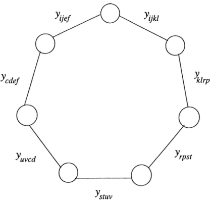
7

, following CCR must be simultaneously satisfied Vijrp ^ E {i = r) V (i = p) (16) Vijst ^ E {i = s) V (i = t) (17) Vijuv ^ E (i = u) V (;■ = u) (18) Vijcd ^ E (f = c) V ( i = d) (19) Vkist ^ E (k = s) V (/ = 0 (20) Vkiuv i E (k = u) V {1 — v) (21) Vkicd i E (k = c) V (l = d) (22) Vklef i E (k = e) V (/ = / ) (23) l/rpuv ^ E (r = ti) V (p = u) (24) Vrpcd ^ E (r = c) V (p — d) (25) Vrpef ^ E (r = e) V (p = / ) (26) Vstcd ^ E (s = c) V {t = d) (27) Vstef ^ E [s = e ) y {t = f ) (28) Vuvef ^ E {u = e) V (u = / ) (29)

and the corresponding (EER) are

Vijki ^ E {i ^ k) A {j ^ /) (30) Vklrp € E ( k ^ r ) A ( l ^ p ) (31) Vrpst £ E =4^ {r ^ s) A { p ^ t) (32) Vstuv ^ E ( s ^ u ) A {tjt: u) (33) Vuvcd £ E {u ^ c) A {v ^ d) (34) Vcdef ^ E => (c e) A (d 7^ / ) (35) Vijef € E {i ^ e ) A {j ^ / ) (36)

CHAPTER 3. QUADRATIC ASSIGNMENT POLYTOPE ₃₁

All the relations listed above must be satisfied simultaneously, i.e. they are connected by an ” and” A operator. Using this fact we will step by step combine the relations into a single binary relation.

Let us start with 16 A 17

(i = r = s) V [(f = r) A (i = t)] V [(i = s)A (j = p)] V (j = p ^ t ) (37) By 32, 37 reduces to

[{i = r) A {j = 0] V [(i = s)A (j = p)] (38) Now, take 18 A 19 (i = u = c) V [(z = c) A (;■ - u)] V [(z = u) A (j = d)] V {j = v d) (39) By 34, 39 reduces to [(z = c) A {j = u)] V [(z = u) A {j = d)] (40) Taking 38 A 40 yields [(i = r = c) A (7 = < = y)] V [(z = r = u) A (j = t = d)]V [(z = s = c) A ( j = p = y)] V [(z = s = u) A { j — p = d)] (41) By 33, 41 reduces to [(i = r = zz) A (j = < = d)] V [(z = 5 = c) A (7 = p = y)j (42) Realize that 42 is equivalent to 16 A 17 A 18 A 19. In a similar way the relations 20, 2 1 , 22 and 23 reduces to

[(¿ = e = z z ) A ( / - t = : : d ) ] V [(¿• = 5 = c ) A ( / = / - y ) ] (43) and the relations 24, 25 and 26 reduces to

[(r = e = u) A (p = d)] V [(r = c) A (p = / = y)] (44) Now, evaluating 42 A 43 yields

CHAPTER 3. QUADRATIC ASSIGNMENT POLYTOPE ₃₂ [{i - r = u) A {j = t = d) A {k = c = s) A {I = f = u)]V [(i = s = c = ^ k ) A { j = l = p = v = /)]V [(i = s = c) A (;■ = p = u) A (fc = e = u) A (/ = c? = i)] (45) By 30, 45 reduces to [{i = r = u) A {j = t = d) A {k = c = s) A {I = f = ■y)]V [(i ~ s — c) A {j = p = v) A {k — e = u) A {I — d — t)] (46)

Finally we evaluate 44 A 46. Realize that 44 A 46 is equivalent to 16 A · · · A 26. [(i = r = u = e) A

(y

= t — d = p) A (k = c = s) A {I = f — u)]V

[{i — s = c ) A { j = p = v = l = d = ^ t ) A{ k — e = u = r)]V

[{i = r = u = k = c — s ) A { j = t = d ) A { l = f = v = p)]V

[{i — s = c = r) A {j = p = V = f ) A {k = e = u) A {I = d = t)] (47)

By 36, 34, 32 47 cannot be realized. Hence, G does not contain chordless cycles o f length 7, i.e.

€7

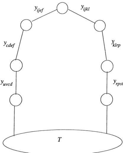
— 0.

T h e o r e m 3.6 The graph G does not contain chordless cycles of length m > 7.

p r o o f:

We will follow a similar method to the previous one. Suppose there exist a

C E Cm where m > 7 and without loss of generality C is shown in figure . We will concentrate on the binary relations over a subset of edges of the C,

over C = {yijki,ykirp,yTpst,yuvcd,ycdef,yijef}· All the previously stated binary relations, 16, · · ·, 36 are still valid with one exception, 33 we do not have edge

ystuv <ii'iy more. There is only one additional requirement

ystuv ^ {s = u) V {t — v) (48) which guarantees the absence of yatuv Again all the binary relations must be satisfied simultaneously, that is, all the binary relations are connected by A operator.

Since 16 A · ■ · A 19 is not affected by the changes, it is equivalent to 42. Also 24 A · · · A 26 is still equivalent to 44.

CHAPTER 3. QUADRATIC ASSIGNMENT POLYTOPE 33

CHAPTER 3. Q UADRATIC ASSIGNMENT POLYTOPE ₃₄ Let us reevaluate 20

A

· · ·

A

23. It is [(^ = 5 = u = c)

A

(/ = / ) ]

V

[(^ = s = [(fe = 5 = c)

A

(/ = u = / ) ]

V [(Ar

= s = [ ( k = u = c) A { 1 = t =

/)] V [(A: = u =

[(A; = c) A (/ = i = u = /)] V [(A: =

By 34, 49 reduces to

[(A- = 5 = u = c) A (/ = /)] V

[(A

= s =

[(A = u = c)

A

(/ = t = / ) ]

V

[(A = Combining 42 with 50 yields

[[i = r = u = k = s = e)A{j = t =

[(z

= r = u ) A ( j = t — d) A ( k = s [(^i = r = u = k = e) A { j — t = d = [(^i = r = u ) A { j = t — d = l = v = [(i = u = k = s = e = c ) A { j = p = [{i = s = c = k) A { j = p — V = I = [(z = s = c) A { j = p = v) A { k = u [{i = s = c = k ) A { j = t = p — 1 = which reduces to

- u =

e) A (l

=

d)]V

--

e) A

(I = V =

d)]V r e) A (/ = < = d)]V e ) A ( l = t ^ v ^ d ) ] (49)

e) A {I — V =

d)]V

e ) A { l

= t = v = d)] (50) d = / ) ] V = c) A (/ = u = /)]V = /)]V

- - f ) A { k

= c)]V = u) A (/ = d)]V /)]V = e) A( l = t —d)]V V = / ) ] (51) [(*■ = r = u) A {j — t = d) A {k — s = c) A (I = V = /)]V [(i = s = c) A (j = p = v) A (k = u = e) A (I = t = d)] (52) by 30, 31, 32, 34, 35 and 36, i.e. edge existence relations. When we combine 52 with 44 we get

[[i = r = u = e) A { j = t = d = p) A {k = s = c) A{1 — V = /)]V

CHAPTER 3. Q UADRATIC ASSIGNMENT POLYTOPE ₀₀

ijkl

yklcd

^cdef

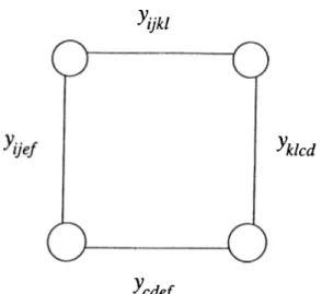
Figure 3.5: Chordless cycle of length 4

[{i = s = c) A {j = p = V = I — t = d) A {k — u = e)]

[[i = s = c = r) A [j = p = V = f ) A {k = u = e) A {I — t — d)] (53) 30 and 36 tells us that 53 cannot be realized. T h e r e f o r e = 0 m = 8,9,10, · · ·. In a similar way it can be shown that G does not contain chordless cycles of length 5 either.

T h e o r e m 3 .7 The graph G contains chordless cycles of length 4 and further­ more for any (7 € C4 folloxuing ch ordless c y c le inequalities are valid for QA^.

Vijki < 1

Vijkl^C

(54)

p r o o f :

Suppose C — {yijkl

1

yklcdt Vcdef iVije/} ·

Edge existence relations (EER) are

Vijkt ^ E yuef ^ E => (i ^ k) A (j / 1) ( i - / e ) A ( ( # / ) (55) (56)

CHAPTER 3. Q UADRATIC ASSIGNMENT PQLYTOPE ₃₆ (c 7^ e) A { d ^ f ) (57) => {i ^ e ) A {j ^ f ) (58) relations (CCR) are (i = c) V (;■ = d) ₍₅₉₎ (k = e) V (l = f ) (60) V cd ei € E y i j c f e E

and respective chordless eye

Uijed ^ E

Vklef ^ E

Evaluating 59 A 60 yields

[(^ = c) A {k = e)] V [(e = c) A (; = / ) ] V [(i = d) A{ k = e)] V [(i = d) A (/ = /) ] (61) 61 is not contradictory with EER. Hence, C4 0 and moreover there are four ways of constructing a C € C4. Validity of chordless cycle inequality 54 follows immediately from the fact that a clique can contain at most one arc from a chordless cycle.

We can show, in a similar way, that also Cq ^ 0. An inequality of the form 54 is dominated by layer constraints 1 1 in the case of C^.

3 .6

B ra n c h and C u t E x p e rim e n ta tio n

In this section we solve the following linear programming relaxation of QAP'^

P r o b le m 3.5

min c^y s.t. Ay = l

l y < l o V ( / , / o ) e £ '

y

> 0

where C is the set of triangle and chordless cycle inequalities for QA'^.

We adopt the Branch and Cut algorithm given by Padberg and Rinaldi [56]. Given a set C , a subset of valid inequalities for QA^ and two disjoint edge sets