Observer based friction cancellation in mechanical systems

2014 14th International Conference on Control, Automation and Systems (ICCAS 2014) Oct. 22-25, 2014 in KINTEX, Gyeonggi-do, Korea

Observer Based Friction Cancellation in Mechanical Systems

Caner Odaba�* and Orner Morgtil

Department of Electrical and Electronics Engineering, Bilkent University, Ankara 06800, Turkey

canero@ee.bilkent.edu.tr, morgul@ee.bilkent.edu.tr * Corresponding author

Abstract: An adaptive nonlinear observer based friction compensation for a special time delayed system is presented in this paper. Considering existing delay, an available Coulomb observer is modified and closed loop system is formed by using a Smith predictor based controller as if the process is delay free. Implemented hierarchical feedback system structure provides two-degree of freedom and controls both velocity and position separately. For this purpose, controller parametrization method is used to extend Smith predictor structure to the position control loop for different types of inputs and disturbance attenuation. Simulation results demonstrate that without requiring much information about friction force, the method can significantly improve the performance of a control system in which it is applied.

Keywords: Time Delay, Smith Predictor Based Controller, Adaptive Observer, Hierarchical Position Control

1. INTRODUCTION

Friction force is one the most important natural nonlin­ earities in mechanical systems and should be considered to design feedback control systems satisfying desired per­ formance criteria such as position tracking. In a simple mechanical system, applied force is control input whereas position and/or velocity is the output. Under the presence of friction, equation of motion can be written as:

lvIi

F+u

(1)

Here, ]v! and i represent the mass and acceleration of moving object respectively,

u

is control input and

F

is friction force. In the absence of

F

acceleration is simply generated by applied

u.

However, presence of

F

leads to performance degradation in the system. In order to over­ come this phenomenon, several different methods can be found in the literature. One popular method is model identification and model based friction compensation [1]. As it is explained in [2], friction can be modeled in vari­ ous complexities. In model based friction compensation techniques, one should firstly identify required parame­ ters of the model. Then, constructed friction model can be added to the system to cancel out

F.

In this approach, it is possible to use a procedure proposed in [3] or [4] to estimate friction parameters. Nevertheless, model param­ eters might not be always identified accurately because of model complexity or measurement errors. Moreover, these parameters can change with time for some physi­ cal reasons such as lubricity, temperature or deformation. Therefore, observer based cancellation techniques can be employed as an alternative. Different kinds of observers are described in [5-8]. However, the observer in [10] is utilized in this article due to its simple structure. Hence, it is easy to modify the observer for the systems with time delay. Furthermore, no matter how complex it is, in most of friction models, Coulomb friction is one of the funda­ mental components of friction force. Hence, the adaptive Coulomb observer in [10] is employed to estimate

fric-tion. Although it is designed to estimate Coulomb fric­ tion, it works well enough for more complex cases and improves the closed loop performance. Besides, original observer design is widely used in the literature to make performance comparisons. Moreover, when velocity is not measurable, second observer is used to estimate the velocity [9].

Likely, time delay can appear very often in many sys­ tems due to transmission, computation or mechanical lags. In such cases, time delay may result in reducing sys­ tem performance, or even cause instability. Since trans­ port delay introduces infinitely many poles to the char­ acteristic equation of the closed loop transfer function, in general it is more difficult to design a stabilizing con­ troller for such systems as compared with the delay free case. Especially, stability margins of the closed loop sys­ tem declines with increasing delay. Therefore, PID con­ trollers are not so efficient when there is long time delay in system dynamics. In 1957, Smith, [11], proposed a particular controller structure employing a feedback loop inside the controller. Using proposed strategy one might design a controller as if the process is delay free. Af­ terwards, many modifications have been proposed to this structure to meet a set of performance and robustness ob­ jectives [12-14]. Using internal model principle, a new Smith predictor based controller is presented in [15] for a special class of plants.

Note that friction terms are not considered in [15] and the delay terms are not considered in the observer struc­ ture proposed in [10]. Motivated by the results given above, in this work we propose a friction cancellation scheme for a class of mechanical systems. Our friction cancellation scheme is based on an adaptive friction ob­ server similar to the one given in [10].

This work is organized as fallows. In the next sec­ tion, we give information on the hierarchical control sys­ tem and its various components. Then, in section 3, we present various simulation results. Finally, we give some

concluding remarks.

2. OVERALL FEEDBACK SYSTEM

In this work, we will consider the hierarchical control system as given in Fig. l.

Fig. 1 Block diagram of overall feedback system In Fig. 1,

P

represents the plant,

F

represents the friction term whereas

P

represents an estimation of the friction; v is the velocity output whereas p represents the

position output. With respect to Eq. (1), v = i; and

p = x. Here,

rp

and

rv

represents position and velocity

command inputs, respectively and d represents the dis­ turbance term acting on the plant. Also

Cv

is a controller which aims at stabilizing the first (inner) loop, which may be called as velocity loop, while

Cp

is another controller which aims at stabilizing the position loop. If one aims at velocity control, the position loop should be switched off, while if one aims at position control, then one should choose

rv

=

O.

2.1 Plant Structure

From the physics in Eq. (1), transfer function of the plant should include an integrator. However, generally, time delay in the system appears due to sampling, sen­ sor/actuator non-collocation, and signal transmission de­ pending on the physical distance between the controller and the plant. Thus, transfer function from input to ve­ locity is in the form

1

P(s)

_e-TdS.

(2)

Ms

where !vI is the mass and

Td

is the delay of the system. Of course, in real systems some higher order dynamics can be occurred; nonetheless, an input filter can be used to suppress them. Hence, we made our simulations using simple plant model in Eq. (2).

2.2 Controller Design for Velocity Loop

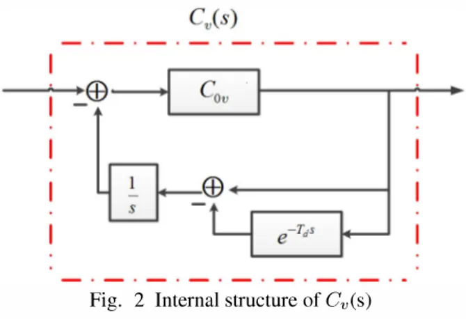
In this section, design methodology described in [15] is brifly mentioned. The structure of

Cv (s)

is illustrated in Fig. 2 and defined as

1

+ Cov(s)

l-es

Td,

• (3) With the defined structures of

Cv(s)

and

P(s),

char­ acteristic equation of closed loop system is

1 1

+ Cov(s)­

s

0,

(4)

---�EB

Fig. 2 Internal structure of

Cv

(s)

which implies that

Cov (s)

must be designed to stabilize an integrator. To find

COv (s),

we utilize the technique proposed in [15].

If the aim is to track the step input without disturbance in the velocity loop, then particular choice would be

(5) Then, closed loop transfer function of the velocity loop,

Tv(s),

would be

Tv(s)

�e-TdS.

s+Kv

(6)

K v

in Eq. (5) is determined by pole placement method considering performance requirements.

If the aim is to track the ramp input without distur­ bance in the velocity loop, then particular choice of

Cov

and closed loop transfer function would be

COv (s)

Tv(s)

2Kvs + K;

s

2Kv8 + K;

e '

-TIS

(s+Kv)2

(7) (8)

To design a controller suppressing constant distur­ bance and tracking step reference signal without a steady­ state error, a particular choice of

Cov

is

and corresponding closed loop transfer function is

Tv(s)

(2Kv + K;Td)S + K;

e-TdS.

(s + Kv)2

(9)

(10)

By using controller parametrization, one can design a different

Cv

to achieve different performance or robust­ ness objectives such as suppressing ramp or sinusoidal disturbance. For detailed analysis, interested reader is re­ ferred to [15].

I

i�

EB

�---+I

:

�:---

�---I

I

�

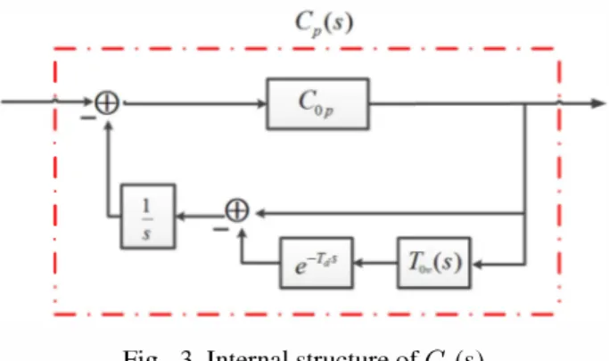
Fig. 3 Internal structure of

Cp(S)

2.3 Controller Design for Position Loop

To design a position controller, structure of velocity controller in Fig. 2 is slightly changed. Fig. 3 is obtained by adding delay free closed loop transfer function for ve­ locity loop to Fig. 2. Let Tov (s) denotes the delay free part ofTv(s).

For position controller,

Cp

(s) given in Fig. 3, same controller structure given in Eq. (5), (7) or (9) can be implemented according to design specifications. Let's consider step reference and constant disturbance rejec­ tion case presented in Eq. (9) which means

(

_{2Kp+Kp s+Kp}

2

)

2

s

-

K�Td

(11)

where

Kp

is a free parameter to be chosen via pole place­ ment like in the velocity loop. Then corresponding trans­ fer function of the overall closed loop feedback system is

T(s)

(2Kp + K;)s + K;

(s

+

Kp)2 Tv(s)' (12)

2.4 Friction Observer Structure

In order to estimate Coulomb friction in a delay free system, Friedland and Park proposed an adaptive ob­ server. Coulomb friction can be defined as

F(v)

(13)

where ac is Coulomb friction parameter. Now consider the system given by Eq. (1) and Eq. (13). The proposed observer in [10] is given by

z-klvllL,

kp, IvllL-

1

(

--

u

- F

)

sgn(v).

!vI (1

4

) (15) Introducing a new state variable

z

and using controller output u, observer aims to estimate ac. In Eq. (1

4

), ac is

estimated friction parameter whereas observer gain

k

and exponent

p,

are design parameters.

Defining an estimation error as

e

:= ac - ac, in [10],

it can be shown easily that error dynamics is given by (16)

For a fixed friction constant ac, Eq, (16) shows that the estimation error converges asymptotically zero when observer gain

k

>

0

and exponent IL >

O.

Since modeled system in Eq. (2) includes a delay term, we modified original observer by adding a delay term as illustrated in Fig.

4.

v ---,---,---,

u

Fig.

4

Modified Coulomb observer.

3. SIMULATION RESULTS

As an example we consider plant

P(

s) given by Eq. (2) with !vI =

5

kg and Td =

0.2

sec. Since real-world

friction may not conform to only Coulomb friction, per­ formance of the observer with more representative model, Eq. (17) is investigated.

F(v)

(

x

+ ye->-Ivl) +

_{z Ivl)sgn(v),}

₍₁₇₎

where x term denotes Coulomb friction whereas

ye->-Ivl)

and

z Ivl

denote Stribeck effect and viscous friction re­ spectively. Viscous friction is a linear function depending on

v.

Thus, it is beneficial to express increase in mag­ nitude of the friction force when velocity is increased. Friction force at rest is generally higher than Coulomb friction. In order to begin moving, one must apply a force greater than Coulomb friction because of the stick friction. After stick friction level is exceeded, friction force decreases smoothly until a certain level. This ef­ fect is called as Stribeck effect. As it is explained in [2], Stribeck effect is used to explain the friction characteris­ tics at low velocities. In Eq. (17), coefficient

y

represents the difference between stick friction and Coulomb fric­ tion while A represents decay rate of friction force due to Stribeck effect. As a whole, Eq. (17) is a similar ex­ pression for steady state behavior of dynamical friction model, LuGre model given in [16].

For our simulations, let us choose x =

5,

y

= 1,

z

= 1

and A = 1 for simplicity. Position loop control with step

input with no disturbance, ramp input with no disturbance and step input with step disturbance are analyzed. In the simulations, we considered three different situations. (i)When there is no friction term in Eq. (1), in this case friction observer is not utilized,

(ii)

when friction exists but observer is not utilized,

(iii)

when friction exists and friction observer is also utilized.

By choosing

Kv

= 1 in Eq. (5) and

Kp

=

3,

per­

formance results of controllers for step tracking without disturbance are plotted in Fig. 5 and Fig. 6 for

k

=

5

and

JL = 1.2. As a result of friction, in friction cancellation,

settling time is slightly increased compared to no friction existence case. However, as it can be observed in Fig. 5, without a compensation both settling time increases a lot and a steady state error about

3%

occurs.

Position Output 1.4,---r---�---�---_.__--_____, 1.2 " � 0.8

1

06 -No Fric Cancellation -No Fric. Case -Fric Cancellation 4 Time (sec)

Fig. 5 Unit step response of the system Moreover, from Fig. 6 it can be deduced that al­ though actual friction does not only include Coulomb friction, observer is capable of estimating it reasonably well enough with a small amount of transition time. In observer parameters, gain

k

determines the speed of esti­ mation. However, increasing it too much results in larger oscillations at the transient; therefore, it might cause to system to be unstable. 10 8 6 4 -2 -4 -6 -8 o

Actual and Estimated Friction Forces

rfl

I

Actual Fric.

-Estimated Fric

10

Time (sec)

Fig. 6 Actual and estimated friction

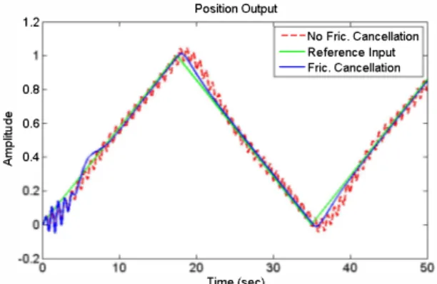
Likewise, tracking performance of proposed system for periodic triangular input with period of 35 sec. is con­ sidered with

Kp

=

5,

Kv

= 1,

k

=

5

and JL = 1.2. As

expected, output is 0.2 sec shifted version of the input. In Fig. 7 it is clear that after an oscillatory transient, can­ cellation matches desired output. However, at direction reversals it needs some time to track the signal in new direction. Nevertheless, without any cancellation there is an oscillatory output causing steady state errors.

In real mechanical systems, it is highly possible that

Position Output 1.2 ---No Fric. Cancellation -Reference Input -Fric. Cancellation 0.8 " "C 0.6 .E I'i E 0.4 -0: -0.20L---,1�0---,2�0---3,.'=0---4�0,---,J50 _{Time (sec)}

Fig. 7 Triangular waveform response of the system

some more disturbance signals other than friction hav­ ing effects on the system performance. Hence, for a unit disturbance rejection and step input tracking controller given by Eq. (9) taking

Kp

=

5,

Kv

= 1,

k

= 1 and

JL = 1.8 is considered. When a relatively large value

of

k

is combined with a large value IL, some "rings " oc­ cur at the output. This situation can be explained by an undesirable sensitivity to disturbance. Thus, considering step tracking case without disturbance, JL is slighlty in­ creased whereas

k

is decreased. From Fig. 8, it is clear that friction cancellation increases system performance under friction. Compared to Fig. (5), existence of unit disturbance makes steady state error larger, at about

5.6%

and oscillations reach steady state after a log time.

Position Output 1.4.---,---,---,---,---, 1.2 � 0.8 . .8 I'i � 06 0.4

0.2 --Fric. Cancellation No Friction

-NoFric. Cancellation

°0�---,�--�170---�1� 5 ======�2�0====�

�

25·

Time (sec)

Fig. 8 Step response of the system with unit disturbance

Furthermore, for different reasons such as tempera­ ture or lubricity, friction coefficients can be time vary­ ing. Hence, observer performance under a friction force whose coefficients are slowly time-varying is also con­ sidered. Clearly, parameters of friction can change in time differently in different systems. Hence, in order to illustrate the response for time varying parameters Eq. (17) is modified to

F

=

(6 + sin(O.05t))sgn(v).

Step tracking without disturbance case is considered with

Kp

= 4,

Kv

= 2,

k

= 4 and JL = 1. In Fig. 9, it is seen

that adaptive observer can estimate time varying parame­ ters.

Actual and Estimated Friction Force 0

I

Actual Friction -Estimated Fric.

If

-r- r--1 '- 7-6 _{20 40 60 80} Time (sec)

F· Ig. 9 Actual and Estimated friction with time varying parameters

4. CONCLUSION

In order to handle with mechanical systems with time delay, Smith predictor based controllers, which are in the form of PI controller, are employed. For different per­ formance and robustness objectives, it is possible to de­ sign controllers via pole placement method. Using a hi­ erarchical closed loop feedback system, performance of an example is analyzed under friction. Thus, adaptive Coulomb observer is modified for mechanical systems with time delay. As expected the mere inclusion of the delay in the observer works well when time delay ex­ ists in system dynamics. Simulations demonstrate that with a proper observer parameter selection it is possible to amend performance criterion such as steady state er­ ror and settling time. Although it is designed to estimate Coulomb friction, results confirm that observer can work well enough for friction models rather than Coulomb fric­ tion. Furthermore, being an adaptive observer, estimation of friction with time varying parameter can be possible.

REFERENCES

[1] H. S. Lee and M. Tomizuka, "Robust motion con­ troller design for high-accuracy positioning sys­ tems, " Industrial Electronics, IEEE Transactions on, vol. 43, no. 1, pp. 48-55, Feb 1996.

[2] H. Olsson, K. strm, C. C. de Wit, M. Gfvert, and P. Lischinsky, "Friction models and friction com­ pensation, " European Journal of Control, vol. 4, no. 3, pp. l76 - 195, 1998.

[3] H. S. Lee and M. Tomizuka, "Robust motion con­ troller design for high-accuracy positioning sys­ tems, " Industrial Electronics, IEEE Transactions on, vol. 43, no. 1, pp. 48-55, Feb 1996.

[4] P. Lischinsky, C. Canudas-De-Wit, and G. Morel, "Friction compensation for an industrial hydraulic robot, " Control Systems, IEEE, vol. 19, no. 1, pp. 25-32, Feb 1999.

[5] S. Tafazoli, C. de Silva, and P. Lawrence, "Track­ ing control of an electrohydraulic manipulator in the presence of friction, " Control Systems Technology, IEEE Transactions on, vol. 6, no. 3, pp. 401-411, May 1998.

[6] W. Chen, K. Kong, and M. Tomizuka, "Hybrid adaptive friction compensation of indirect drive trains, " in ASME 2009 Dynamic Systems and Con­ trol Conference. American Society of Mechanical Engineers, 2009, pp. 313-320.

[7] Q. P. Ha, A. Bonchis, D. C. Rye, and H. F. Durrant-Whyte, "Variable structure systems ap­ proach to friction estimation and compensation, " in Robotics and Automation, 2000. Proceedings. ICRA '00. IEEE International Conference on, vol. 4. IEEE, 2000, pp. 3543-3548.

[8] W.-H. Chen, D. Ballance, P. Gawthrop, and J. O'Reilly, "A nonlinear disturbance observer for robotic manipulators, " Industrial Electronics, IEEE Transactions on, vol. 47, no. 4, pp. 932-938, Aug 2000.

[9] S. Mentzelopoulou and B. Friedland, "Experimen­ tal evaluation of friction estimation and compensa­ tion techniques, " in American Control Conference, 1994, vol. 3, .Tune 1994, pp. 3132-3136 vol.3. [10] B. Friedland and Y-J. Park, "On adaptive friction

compensation, " Automatic Control, IEEE Transac­ tions on, vol. 37, no. 10, pp. 1609-1612, Oct 1992. [11] O. J. Smith, "Closer control of loops with dead time, " Chemical Engineering Progress, vol. 53, no. 5, pp. 217-219, 1957.

[12] K.-S. Hong, D.-H. Kang, and .T.-G. Kim, "Robust smith predictor design via uncertainty quantifica­ tion: Application to a reclaimer, " IFAC System Iden­ tification, 2000.

[13] M. Matausek and A. Micic, "A modified smith pre­ dictor for controlling a process with an integra­ tor and long dead-time, " Automatic Control, IEEE Transactions on, vol. 41, no. 8, pp. 1199-1203, Aug 1996.

[14] A. Visioli and Q.-C. Zhong, "Smith-predictor-based control, " in Control of Integra I Processes with Dead Time, ser. Advances in Industrial Control. Springer London, 2011, pp. 141-185.

[15] U. Tasdelen and H. Ozbay, "On smith predictor­ based controller design for systems with integral action and time delay, " in Control Conference (ASCC), 2013 9th Asian, June 2013, pp. 1-6. [16] c. de Wit, H. Olsson, K. Astrom, and P. Lischinsky,

"A new model for control of systems with friction, " Automatic Control, IEEE Transactions on, vol. 40, no. 3, pp. 419-425, Mar 1995.