Ground-state properties of quasi-one-dimensional electron systems within dynamic
local-field correction: Quantum Singwi-Tosi-Land-Sjo¨lander theory
B. Tanatar
Department of Physics, Bilkent University, Bilkent, 06533 Ankara, Turkey
C. Bulutay
Department of Electrical and Computer Engineering, University of California, Santa Barbara, California 93106 and Department of Electrical and Electronics Engineering, Middle East Technical University, 06531 Ankara, Turkey
~Received 16 November 1998!
Dynamic local-field correction~LFC! brings a richer picture about the description of a many-body system than the standard mean-field theories. Here we investigate the ground-state properties of a quasi-one-dimensional electronic system using the quantum version of the Singwi-Tosi-Land-Sjo¨lander~STLS! theory and present a critical account of its performance. The results are markedly different than those theories based on static LFC and the random-phase approximation; an example is the static structure factor, which develops a significant peak at low densities, signaling a developing ordered phase. An indication of growing instability at low densities is seen on G(q,0), the static behavior of the dynamic LFC, which has an oscillatory character with a magnitude exceeding unity, peaking exactly at 4kF. The pair-correlation function comes out as positive for the densities considered in this work. The correlation energy and the compressibility curves are seen to be quite close to the static STLS results. A flaw of the theory is the significantly negative values of the dynamic structure factor around the plasmon frequencies, also the lifetime of the plasmons turns out to be negative away from the single-pair continuum. In summary, the major shortcomings of the dynamic STLS scheme are the violation of the compressibility sum rule~as in the static STLS case! and the misrepresentation of the plasmons in the dynamic structure factor.@S0163-1829~99!00324-0#
I. INTRODUCTION
Quantum confinement as in quasi-one-dimensional~Q1D! electronic systems, increases the role played by the many-body effects. As opposed to the Tomonaga-Luttinger liquid model1,2for the Q1D systems, Hu and Das Sarma3 showed that in the presence of small disorder or finite temperature the Fermi surface is restored. This finding reassured the use of Fermi-liquid models4 for characterizing Q1D systems. In particular, random-phase approximation ~RPA!4–6 and its improvements by including the static local-field correction ~LFC!, such as in the Singwi-Tosi-Land-Sjo¨lander ~STLS! approach7have been applied to Q1D systems.8–13 Consider-ing its performance in higher-dimensional systems as well, RPA is known to be successful in one-electron properties,6 such as the self-energy and its end-products like band-gap renormalization and quasiparticle lifetime. Furthermore, the behavior of collective excitations ~plasmons in this case! is seen to be quantitatively reproduced by RPA,8offering much better agreement with experiment14 compared to its ‘‘im-proved’’ versions including LFC. However, from other many-body aspects, and in particular for the pair-correlation function, RPA gives grossly unphysical results,7 which be-come worse as the dimensionality is reduced;15this artifact is directly carried over to the correlation energy results as well. In this regard, correlation energy functional of a many-body system happens to be an important input to the recent quan-tum freezing theories,16,17as has been demonstrated very re-cently on the estimation of Wigner crystallization density in quantum wires.18On the other hand, approaches having LFC such as STLS are successful in reproducing the
pair-correlation function and pair-correlation energy results of the quantum Monte Carlo ~QMC! simulations from high densi-ties to moderate densidensi-ties; however, low-density perfor-mance is unsatisfactory,19and the violation of the compress-ibility sum rule over all densities is another problem shared with RPA.
A common viewpoint is the need to incorporate dynami-cal correlations to capture the full many-body physics. Spe-cifically, the importance of dynamical local fields is evident from various applications such as construction of effective electron-electron interactions20that are relevant for Coulomb interaction induced superconductivity, electronic energy-loss straggling of protons in the electron gas,21 determining the plasmon lifetime, and setting up the exchange-correlation potential in the context of time-dependent density-functional theory.22 One of the pioneering works, offering a dynamic LFC is that of Hasegawa and Shimizu,23where they replaced the original STLS LFC scheme by a full quantum-mechanical framework with the use of Wigner distribution function. Their approach directly leads to a dynamic LFC and is usually named as the quantum STLS ~QSTLS! or sometimes as the dynamic STLS. Later, Holas and Rahman reported a detailed numerical account of the QSTLS in three-dimensional ~3D! electron liquid ~EL!,24 Moudgil et al. ap-plied QSTLS to 2D EL examining the spin-density response as well.25For the remaining Q1D EL, very recently we have investigated the performance of QSTLS, focusing mainly on the static properties.26Our aim in the present work is to bring the level of the current understanding about the performance of QSTLS to those of higher dimensions.24,25With this mo-tivation, we give a critical account of the QSTLS in Q1D, PRB 59
which we hope to be useful in the advancement of dynamic LFC schemes.
The outline of this paper is as follows. In Sec. II, we give the theoretical formalism of the self-consistent QSTLS equa-tions, as well as the correlation energy and compressibility expressions. In Sec. III, we present the ground-state proper-ties of the Q1D electronic systems using QSTLS theory, oc-casionally comparing with mainly the STLS results. In Sec. IV, we gather our assessment of the performance of the QSTLS for the Q1D electronic systems.
II. THEORETICAL FORMALISM A. Self-consistent equations
The density response to a longitudinal perturbation coupled to density is governed by the longitudinal density-density response function,x(q,v).4This quantity has central importance in characterizing a many-body system. The density-density response function beyond the RPA frame-work is usually taken to be of the form27
x~q,v!5 x
0~q,v!
12U0~q!@12G~q,v!#x0~q,v!, ~1! where G(q,v) is the frequency- and wave-number-dependent LFC, representing the Pauli and Coulomb holes around each electron within the system, x0(q,v) is the density-density response function of the noninteracting sys-tem ~here Q1D EL!, U0(q) is the bare interaction potential for the Q1D EL. We model the Q1D EL as obtained from the zero-thickness 2D EL under a confining potential.28 This yields U0(q)5(e2/e
0)exK0(x) for the Coulomb interaction between the electrons assumed to be in the lowest subband. Here x5(bq/2)2, where b is the lateral width of the quantum wire determined by the confining oscillator frequency, and
e0 is the background dielectric constant. The system is char-acterized by the dimensionless density parameter rs5a/aB*,
where a is the average interparticle distance~i.e., n51/2a in terms of the linear number density n), and aB*5e0/(m*e2) is the effective Bohr radius ~we take \51). The single-subband approximation, which implies that the Fermi energy remains smaller than the intersubband energy difference, is justified for rs.(p/25/2)(b/aB*). Since we have reported
re-sults for b52aB* only, in an earlier publication,26 here we explore the dependence of various quantities on the width parameter. In this theoretical formalism section, we use nor-malized quantities for the wave number and energy, with the normalization being kF ~Fermi wave number! and 2EF (EF
is the Fermi energy!, respectively. We include disorder ef-fects into our treatment within the simple number-conserving Mermin-Das scheme.29 Accordingly, the density-density re-sponse function of the noninteracting system with disorder is given by xg0~q,v!5 ~v1ig!x0~q,v1ig! v1igx 0~q,v1ig! x0~q,0! , ~2!
hereg is the disorder parameter, which we take throughout this work as 0.05 ~in units of 2EF). For the dynamic LFC,
the quantum version23 of the original STLS approach7 is used, which is given by
G~q,iv!51 4
E
0 ` dq8
xg 0~q,q8
;iv! xg0~q,iv! U0~q8
! U0~q! 3@S~q1q8
!2S~uq2q8
u!#. ~3! As in the 2D counterpart,25 we work in the imaginary fre-quency formalism to facilitate the subsequent calculations. In Eq. ~3!, xg0(q,q8
;iv) is the inhomogeneous density-density response function given explicitly for the disorder-free case as x0~q,q8
;iv!5 m* pkF 1 qlnF
v21v 2~q,q8
!2 v21v 1~q,q8
!2G
, ~4!where m* is the electron effective mass, and v6(q,q
8
) 5uq(16q8
/2)u. For the expression ofxg0(q,q8
;iv) with dis-order, we similarly adapt Eq. ~2! of the homogeneous case.S(q) in Eq.~3! is the static structure factor, which is related
to the density-density response function through the fluctuation-dissipation theorem as S~q!52 1 np
E
0 ` dv xg~q,iv!, ~5! 52 1 npE
0 ` dv xg 0~q,iv! 12U0~q!xg0~q,iv!@12G~q,iv!#. ~6! The primary advantage of analytic continuation of the re-sponse function to the complex frequency plane followed by Wick rotation of the frequency integral30 is the robust cap-ture of the plasmon contribution, which dominates in Q1D case. However, in its present form the integrand becomes slowly converging. As a remedy, to Eq. ~5!, we add and subtract the Hartree-Fock static structure factorSHF~q!5 1 2p
E
0 ` dv1 qlnF
v21q2~12q/2!2 v21q2~11q/2!2G
~7! with its closed form being SHF(uqu,2)5uqu/2 and SHF(uqu .2)51, which then results in a rapidly decaying integrand. Using limv→`x0(q,q8
;iv)/x0(q,iv)5limv→`x0(q,q
8
;v)/x0(q,v)5q8
/q, we get lim v→` G~q,iv!5G~q,i`!5G~q,`!, ~8! 51 4E
0 ` dq8
q8
q U0~q8
! U0~q! @S~q1q8
!2S~uq2q8
u!#. ~9!Note that G(q,`) formally reduces to the expression satis-fied by the STLS LFC, G(q). Furthermore, the behavior for largev is of the form G(q,iv)5G(q,`)1O(v22). Based on this behavior, we compute G(q,iv) up to a large value of
G~q,iv!.G~q,`!1
S
vLv
D
2
@G~q,ivL!2G~q,`!#.
~10! Equations~3! and ~5! are to be solved self-consistently. Note that G(q,iv) is real, whereas the dynamic LFC along the real frequency axis G(q,v) is complex, which can be ob-tained from the former by the analytic continuation iv→v 1ih.
Finally, the pair-correlation function is the Fourier trans-form of the static structure factor
g~r!5121
2
E
0`
dq cos~qr!@12S~q!#, ~11!
where, in the same spirit of normalization used throughout this section, distance r above is in units of 1/kF.
B. Correlation energy and compressibility
The correlation energy is the improvement in the ground-state energy of the many-body system over the Hartree-Fock estimate. The common approach is to calculate it via the coupling-constant integration.6 The alternative is Rice’s approach,31 which has been revived recently,32,13where the correlation energy at a density rsis given by
Ec~Ry*!5 p 32rs2
E
0 ` dqE
0 ` dv 3S
ln$12U 0~q!@12G~q,iv!#x g 0~q,iv!% 12G~q,iv! 1U0~q!x g 0~q,iv!D
. ~12! The exchange energy is given byEx~Ry*!52
1 4rs
E
0`
dq F~q!@12q/2#, ~13!
where F(q)5U0(q)/(e2/e0). Both the exchange and corre-lation energy above are in 3D effective Rydberg units @Ry*5m*e4/(2e02)#.
Isothermal compressibility is an important quantity as it challenges the approaches ~including both RPA and STLS! via the compressibility sum rule. This sum rule requires the compressibility computed in two different ways to agree;6 namely, compressibility is obtained by the second derivative of the energy and also by the long-wavelength behavior of the static dielectric function. In the former one, the inverse compressibility normalized to that of the noninteracting Fermi gas value (k0) is given by
k0
k 511
8rs4
p2 d2
drs2@Ex~Ry*!1Ec~Ry*!#, ~14!
whereas the alternative expression obtained via the long-wavelength static dielectric function, limq→0e(q,0), leads to
k0 k 511 4rs p2
E
0 ` dq F~q!lnU
22q 21qU
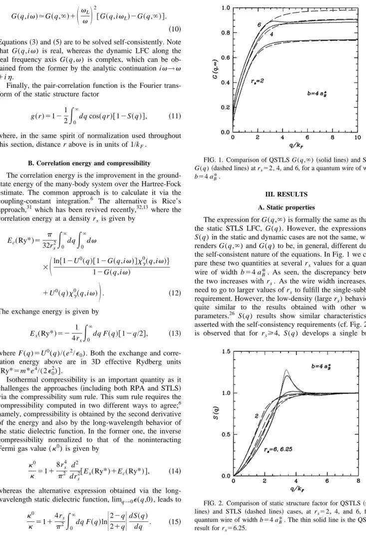
dS~q! dq . ~15! III. RESULTS A. Static propertiesThe expression for G(q,`) is formally the same as that of the static STLS LFC, G(q). However, the expressions for
S(q) in the static and dynamic cases are not the same, which
renders G(q,`) and G(q) to be, in general, different due to the self-consistent nature of the equations. In Fig. 1 we com-pare these two quantities at several rs values for a quantum
wire of width b54 aB*. As seen, the discrepancy between the two increases with rs. As the wire width increases, we
need to go to larger values of rsto fulfill the single-subband
requirement. However, the low-density~large rs) behavior is
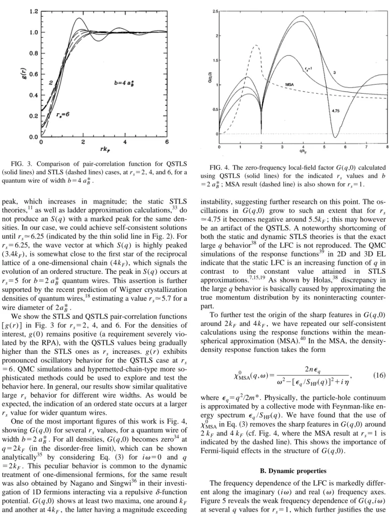
quite similar to the results obtained with other width parameters.26 S(q) results show similar characteristics, as
asserted with the self-consistency requirements~cf. Fig. 2!. It is observed that for rs>4, S(q) develops a single broad
FIG. 1. Comparison of QSTLS G(q,`) ~solid lines! and STLS G(q)~dashed lines! at rs52, 4, and 6, for a quantum wire of width b54 aB*.
FIG. 2. Comparison of static structure factor for QSTLS~solid lines! and STLS ~dashed lines! cases, at rs52, 4, and 6, for a quantum wire of width b54 aB*. The thin solid line is the QSTLS result for rs56.25.
peak, which increases in magnitude; the static STLS theories,11as well as ladder approximation calculations,33do not produce an S(q) with a marked peak for the same den-sities. In our case, we could achieve self-consistent solutions until rs.6.25 ~indicated by the thin solid line in Fig. 2!. For
rs56.25, the wave vector at which S(q) is highly peaked
(3.4kF), is somewhat close to the first star of the reciprocal lattice of a one-dimensional chain (4kF), which signals the
evolution of an ordered structure. The peak in S(q) occurs at
rs55 for b52 aB* quantum wires. This assertion is further supported by the recent prediction of Wigner crystallization densities of quantum wires,18estimating a value rs.5.7 for a
wire diameter of 2aB*.
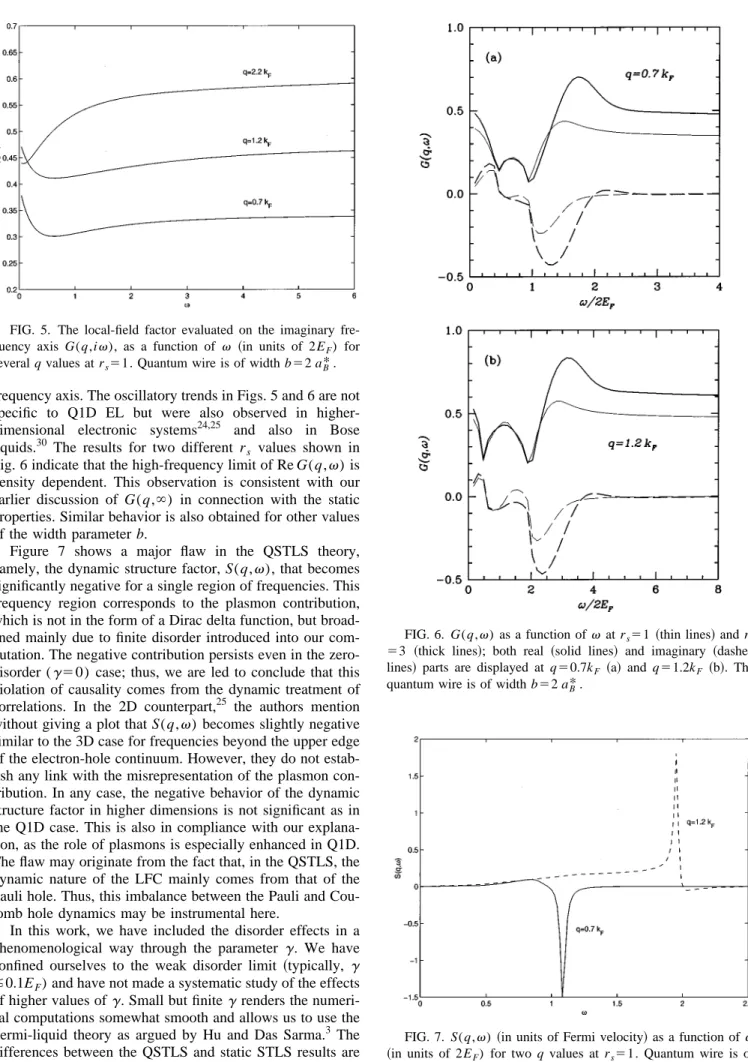
We show the STLS and QSTLS pair-correlation functions @g(r)# in Fig. 3 for rs52, 4, and 6. For the densities of
interest, g(0) remains positive~a requirement severely vio-lated by the RPA!, with the QSTLS values being gradually higher than the STLS ones as rs increases. g(r) exhibits
pronounced oscillatory behavior for the QSTLS case at rs
56. QMC simulations and hypernetted-chain-type more so-phisticated methods could be used to explore and test the behavior here. In general, our results show similar qualitative large rs behavior for different wire widths. As would be
expected, the indication of an ordered state occurs at a larger
rs value for wider quantum wires.
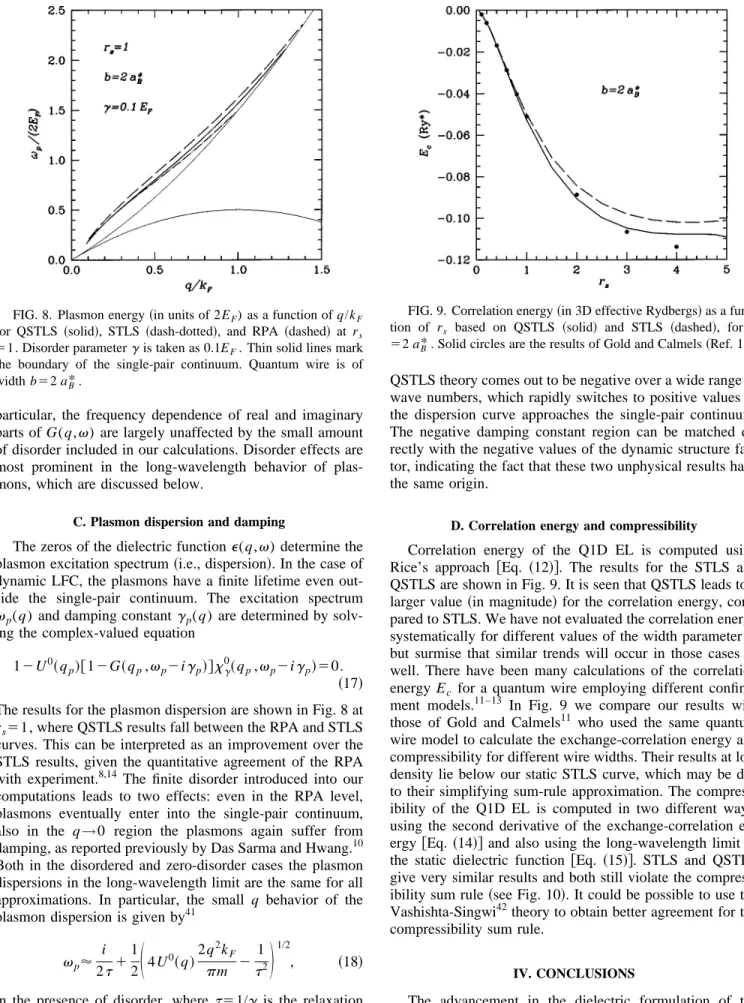
One of the most important figures of this work is Fig. 4, showing G(q,0) for several rsvalues, for a quantum wire of width b52 aB*. For all densities, G(q,0) becomes zero34 at
q52kF ~in the disorder-free limit!, which can be shown
analytically35 by considering Eq. ~3! for iv50 and q 52kF. This peculiar behavior is common to the dynamic
treatment of one-dimensional fermions, for the same result was also obtained by Nagano and Singwi36 in their investi-gation of 1D fermions interacting via a repulsived-function potential. G(q,0) shows at least two maxima, one around kF
and another at 4kF, the latter having a magnitude exceeding
unity appreciably. Gasser37 attributed the 4kF instability in
Q1D systems to multipair excitations. QSTLS does not in-clude multipair excitations but surprisingly still signals a 4kF
instability, suggesting further research on this point. The os-cillations in G(q,0) grow to such an extent that for rs
.4.75 it becomes negative around 5.5kF; this may however
be an artifact of the QSTLS. A noteworthy shortcoming of both the static and dynamic STLS theories is that the exact large q behavior38of the LFC is not reproduced. The QMC simulations of the response functions39 in 2D and 3D EL indicate that the static LFC is an increasing function of q in contrast to the constant value attained in STLS approximations.7,15,19 As shown by Holas,38 discrepancy in the large q behavior is basically caused by approximating the true momentum distribution by its noninteracting counter-part.
To further test the origin of the sharp features in G(q,0) around 2kF and 4kF, we have repeated our self-consistent
calculations using the response functions within the mean-spherical approximation~MSA!.40 In the MSA, the density-density response function takes the form
xMSA
0 ~q,v!5 2neq
v22@e
q/SHF~q!#21ih
, ~16!
where eq5q2/2m*. Physically, the particle-hole continuum
is approximated by a collective mode with Feynman-like en-ergy spectrum eq/SHF(q). We have found that the use of
xMSA 0
in Eq.~3! removes the sharp features in G(q,0) around 2 kF and 4 kF ~cf. Fig. 4, where the MSA result at rs51 is
indicated by the dashed line!. This shows the importance of Fermi-liquid effects in the structure of G(q,0).
B. Dynamic properties
The frequency dependence of the LFC is markedly differ-ent along the imaginary (iv) and real (v) frequency axes. Figure 5 reveals the weak frequency dependence of G(q,iv) at several q values for rs51, which further justifies the use
of imaginary frequency approach in self-consistent equa-tions. The real and imaginary parts of G(q,v) are contained in Fig. 6, displaying oscillatory dependence along the real FIG. 3. Comparison of pair-correlation function for QSTLS
~solid lines! and STLS ~dashed lines! cases, at rs52, 4, and 6, for a quantum wire of width b54 aB*.
FIG. 4. The zero-frequency local-field factor G(q,0) calculated using QSTLS ~solid lines! for the indicated rs values and b 52 aB*; MSA result~dashed line! is also shown for rs51.
frequency axis. The oscillatory trends in Figs. 5 and 6 are not specific to Q1D EL but were also observed in higher-dimensional electronic systems24,25 and also in Bose liquids.30 The results for two different rs values shown in
Fig. 6 indicate that the high-frequency limit of Re G(q,v) is density dependent. This observation is consistent with our earlier discussion of G(q,`) in connection with the static properties. Similar behavior is also obtained for other values of the width parameter b.
Figure 7 shows a major flaw in the QSTLS theory, namely, the dynamic structure factor, S(q,v), that becomes significantly negative for a single region of frequencies. This frequency region corresponds to the plasmon contribution, which is not in the form of a Dirac delta function, but broad-ened mainly due to finite disorder introduced into our com-putation. The negative contribution persists even in the zero-disorder (g50) case; thus, we are led to conclude that this violation of causality comes from the dynamic treatment of correlations. In the 2D counterpart,25 the authors mention without giving a plot that S(q,v) becomes slightly negative similar to the 3D case for frequencies beyond the upper edge of the electron-hole continuum. However, they do not estab-lish any link with the misrepresentation of the plasmon con-tribution. In any case, the negative behavior of the dynamic structure factor in higher dimensions is not significant as in the Q1D case. This is also in compliance with our explana-tion, as the role of plasmons is especially enhanced in Q1D. The flaw may originate from the fact that, in the QSTLS, the dynamic nature of the LFC mainly comes from that of the Pauli hole. Thus, this imbalance between the Pauli and Cou-lomb hole dynamics may be instrumental here.
In this work, we have included the disorder effects in a phenomenological way through the parameter g. We have confined ourselves to the weak disorder limit ~typically, g &0.1EF) and have not made a systematic study of the effects
of higher values ofg. Small but finiteg renders the numeri-cal computations somewhat smooth and allows us to use the Fermi-liquid theory as argued by Hu and Das Sarma.3 The differences between the QSTLS and static STLS results are mostly due to the dynamic nature of the local-field factors. In FIG. 5. The local-field factor evaluated on the imaginary fre-quency axis G(q,iv), as a function of v ~in units of 2EF) for several q values at rs51. Quantum wire is of width b52 aB*.
FIG. 6. G(q,v) as a function of v at rs51 ~thin lines! and rs 53 ~thick lines!; both real ~solid lines! and imaginary ~dashed lines! parts are displayed at q50.7kF ~a! and q51.2kF ~b!. The quantum wire is of width b52 aB*.
FIG. 7. S(q,v) ~in units of Fermi velocity! as a function of v ~in units of 2EF) for two q values at rs51. Quantum wire is of width b52 aB*.
particular, the frequency dependence of real and imaginary parts of G(q,v) are largely unaffected by the small amount of disorder included in our calculations. Disorder effects are most prominent in the long-wavelength behavior of plas-mons, which are discussed below.
C. Plasmon dispersion and damping
The zeros of the dielectric functione(q,v) determine the plasmon excitation spectrum~i.e., dispersion!. In the case of dynamic LFC, the plasmons have a finite lifetime even out-side the single-pair continuum. The excitation spectrum
vp(q) and damping constantgp(q) are determined by
solv-ing the complex-valued equation 12U0~qp!@12G~qp,vp2igp!#xg
0~q
p,vp2igp!50.
~17! The results for the plasmon dispersion are shown in Fig. 8 at
rs51, where QSTLS results fall between the RPA and STLS
curves. This can be interpreted as an improvement over the STLS results, given the quantitative agreement of the RPA with experiment.8,14 The finite disorder introduced into our computations leads to two effects: even in the RPA level, plasmons eventually enter into the single-pair continuum, also in the q→0 region the plasmons again suffer from damping, as reported previously by Das Sarma and Hwang.10 Both in the disordered and zero-disorder cases the plasmon dispersions in the long-wavelength limit are the same for all approximations. In particular, the small q behavior of the plasmon dispersion is given by41
vp' i 2t1 1 2
S
4U 0~q!2q 2k F pm 2 1 t2D
1/2 , ~18!in the presence of disorder, where t51/g is the relaxation time. There exists a critical wave vector below which plas-mons cannot propagate as discussed by Das41 and recently by Das Sarma and Hwang.10 The damping constant of the
QSTLS theory comes out to be negative over a wide range of wave numbers, which rapidly switches to positive values as the dispersion curve approaches the single-pair continuum. The negative damping constant region can be matched di-rectly with the negative values of the dynamic structure fac-tor, indicating the fact that these two unphysical results have the same origin.
D. Correlation energy and compressibility
Correlation energy of the Q1D EL is computed using Rice’s approach @Eq. ~12!#. The results for the STLS and QSTLS are shown in Fig. 9. It is seen that QSTLS leads to a larger value ~in magnitude! for the correlation energy, com-pared to STLS. We have not evaluated the correlation energy systematically for different values of the width parameter b, but surmise that similar trends will occur in those cases as well. There have been many calculations of the correlation energy Ec for a quantum wire employing different
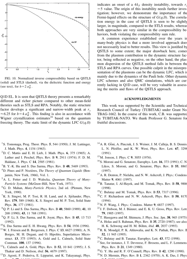
confine-ment models.11–13 In Fig. 9 we compare our results with those of Gold and Calmels11 who used the same quantum wire model to calculate the exchange-correlation energy and compressibility for different wire widths. Their results at low density lie below our static STLS curve, which may be due to their simplifying sum-rule approximation. The compress-ibility of the Q1D EL is computed in two different ways: using the second derivative of the exchange-correlation en-ergy@Eq. ~14!# and also using the long-wavelength limit of the static dielectric function @Eq. ~15!#. STLS and QSTLS give very similar results and both still violate the compress-ibility sum rule~see Fig. 10!. It could be possible to use the Vashishta-Singwi42theory to obtain better agreement for the compressibility sum rule.
IV. CONCLUSIONS
The advancement in the dielectric formulation of the many-body problem relies on the dynamic LFC schemes. A promising candidate in this respect is the QSTLS theory, and in this work we investigate its performance for the case of FIG. 8. Plasmon energy~in units of 2EF) as a function of q/kF
for QSTLS ~solid!, STLS ~dash-dotted!, and RPA ~dashed! at rs 51. Disorder parameterg is taken as 0.1EF. Thin solid lines mark the boundary of the single-pair continuum. Quantum wire is of width b52 aB*.
FIG. 9. Correlation energy~in 3D effective Rydbergs! as a func-tion of rs based on QSTLS ~solid! and STLS ~dashed!, for b 52 aB*. Solid circles are the results of Gold and Calmels~Ref. 11!.
Q1D EL. It is seen that QSTLS theory presents a remarkably different and richer picture compared to other mean-field theories such as STLS and RPA. Notably, the static structure factor develops a significant and narrow-width peak at rs
'6.25 for b54 aB*. This finding is also in accordance with
Wigner crystallization estimates18 based on the quantum freezing theory. The static limit of the dynamic LFC G(q,0)
indicates an onset of a 4kF density instability, towards rs
55 value. The origin of this instability needs further inves-tigation; however, we demonstrate the importance of the Fermi-liquid effects on the structure of G(q,0). The correla-tion energy in the case of QSTLS is seen to be slightly larger, in magnitude, compared to the STLS results, whereas both approaches are very similar in the compressibility be-haviors, both violating the compressibility sum rule.
A common experience established over the years in many-body physics is that a more involved approach does not necessarily lead to better results. This view is justified by QSTLS to some extent; the major drawback here, comes from the plasmon contribution to the dynamic structure fac-tor, being reflected as negative, on the other hand, the plas-mon dispersion of the QSTLS method falls in between the STLS and RPA curves. One possible culprit in the misrepre-sentation of the plasmons can be the dynamic LFC, which is mainly due to the dynamics of the Pauli hole. Other dynamic LFC schemes and also QMC simulations, which are cur-rently lacking in Q1D case, will be very valuable in assess-ing the merits and flaws of the QSTLS approach.
ACKNOWLEDGMENTS
This work was supported by the Scientific and Technical Research Council of Turkey ~TUBITAK! under Grant No. TBAG-1662. In the course of this work, C.B. was supported by TUBITAK-NATO. We thank Professor G. Senatore for fruitful discussions.
1S. Tomonaga, Prog. Theor. Phys. 5, 544~1950!; J. M. Luttinger,
J. Math. Phys. 4, 1154~1963!.
2D. C. Mattis and E. H. Lieb, J. Math. Phys. 6, 375~1965!; A.
Luther and I. Peschel, Phys. Rev. B 9, 2911 ~1974!; F. D. M. Haldane, J. Phys. C 14, 2585~1981!.
3B. Y.-K. Hu and S. Das Sarma, Phys. Rev. B 48, 5469~1993!. 4D. Pines and P. Nozie`res, The Theory of Quantum Liquids
~Ben-jamin, New York, 1966!, Vol. 1.
5A. L. Fetter and J. D. Walecka, Quantum Theory of
Many-Particle Systems~McGraw-Hill, New York, 1971!.
6G. D. Mahan, Many-Particle Physics, 2nd ed. ~Plenum, New
York, 1990!.
7K. S. Singwi, M. P. Tosi, R. H. Land, and A. Sjo¨lander, Phys.
Rev. 179, 589~1968!; K. S. Singwi and M. P. Tosi, Solid State Phys. 36, 177~1981!.
8Q. P. Li and S. Das Sarma, Phys. Rev. B 40, 5860~1989!; 41, 10
268~1990!; 43, 11 768 ~1991!.
9Q. P. Li, S. Das Sarma, and R. Joynt, Phys. Rev. B 45, 13 713
~1992!.
10S. Das Sarma and E. H. Hwang, Phys. Rev. B 54, 1936~1996!. 11W. I. Friesen and B. Bergersen, J. Phys. C 13, 6627~1980!; A. N.
Borges, M. H. Degani, and O. Hipolito, Superlattices Micro-struct. 13, 375 ~1993!; A. Gold and L. Calmels, Solid State Commun. 100, 137~1996!.
12L. Calmels and A. Gold, Phys. Rev. B 52, 10 841~1995!; J. S.
Thakur and D. Neilson, ibid. 56, 4679~1997!.
13D. Agosti, F. Pederiva, E. Lipparini, and K. Takayanagi, Phys.
Rev. B 57, 14 869~1998!.
14A. R. Go˜ni, A. Pinczuk, J. S. Weiner, J. M. Calleja, B. S. Dennis,
L. N. Pfeiffer, and K. W. West, Phys. Rev. Lett. 67, 3298 ~1991!.
15M. Jonson, J. Phys. C 9, 3055~1976!.
16S. Moroni and G. Senatore, Europhys. Lett. 16, 373~1991!; C. N.
Likos, S. Moroni, and G. Senatore, Phys. Rev. B 55, 8867 ~1997!.
17A. R. Denton, P. Nielaba, and N. W. Ashcroft, J. Phys.: Condens.
Matter 9, 4061~1997!.
18B. Tanatar, I. Al-Hayek, and M. Tomak, Phys. Rev. B 58, 9886
~1998!.
19C. Bulutay and M. Tomak, Phys. Rev. B 53, 7317~1996!. 20C. F. Richardson and N. W. Ashcroft, Phys. Rev. B 50, 8170
~1994!.
21N. P. Wang, J. Phys.: Condens. Matter 9, 6837~1997!.
22J. F. Dobson, M. J. Bu¨nner, and E. K. U. Gross, Phys. Rev. Lett.
79, 1905~1997!.
23T. Hasegawa and M. Shimuzu, J. Phys. Soc. Jpn. 38, 965~1975!. 24A. Holas and S. Rahman, Phys. Rev. B 35, 2720~1987!; see also,
H. K. Schweng and H. M. Bo¨hm, ibid. 48, 2037~1993!.
25R. K. Moudgil, P. K. Ahluwalia, and K. N. Pathak, Phys. Rev. B
52, 11 945~1995!.
26
C. Bulutay and B. Tanatar, Europhys. Lett. 43, 572~1998!.
27See, for instance, J. T. Devreese, F. Brosens, and L. F. Lemmens,
Phys. Rev. B 21, 1349~1980!.
28G. Y. Hu and R. F. O’Connell, Phys. Rev. B 42, 1290~1990!. 29N. D. Mermin, Phys. Rev. B 1, 2362~1970!; A. K. Das, J. Phys.
F 5, 2035~1975!. FIG. 10. Normalized inverse compressibility based on QSTLS
~solid! and STLS ~dashed!, via the dielectric function and energy ~see text!, for b52 aB*.
30K. Tankeshwar, B. Tanatar, and M. P. Tosi, Phys. Rev. B 57,
8854~1998!.
31T. M. Rice, Ann. Phys.~N.Y.! 31, 100 ~1965!. 32
F. Pederiva, E. Lipparini, and K. Takayanagi, Europhys. Lett. 40, 607~1997!.
33N. Nafari and B. Davoudi, Phys. Rev. B 57, 2447 ~1998!; L.
Calmels and A. Gold, ibid. 57, 1436~1998!.
34In our previous work ~Ref. 26!, G(q,0) had a dip at q52kF
without reaching zero value. This stemmed from using v 50.02 EFvalue rather thanv50, due to numerical concerns in that computation. This is the reason for the minor discrepancy between G(q,0) results presented here and in Ref. 26.
35The vanishing of G(2k
F,0) can most easily be seen by
consider-ing the ratiox0(2kF,k;0)/x
0
(2kF,0), which appears in the in-tegrand@Eq. ~3!#. At q52kF, the denominator tends to infinity while the numerator remains finite.
36
S. Nagano and K. S. Singwi, Phys. Rev. B 27, 6732~1983!.
37W. Gasser, Solid State Commun. 56, 121~1985!.
38A. Holas, in Strongly Coupled Plasma Physics, edited by F. J.
Rogers and H. E. DeWitt~Plenum, New York, 1987!.
39S. Moroni, D. M. Ceperley, and G. Senatore, Phys. Rev. Lett. 69,
1837~1992!; 75, 689 ~1995!.
40See, for instance, N. Iwamoto, E. Krotscheck, and D. Pines, Phys.
Rev. B 29, 3936~1984!.
41A. K. Das, J. Phys. F 16, L99~1986!.