REASONING FOR ROBOTIC PLANNING
WITHIN THE TWELF LOGICAL
FRAMEWORK AND THE PROLOG
LANGUAGE
a thesis
submitted to the department of computer engineering
and the institute of engineering and science
of bilkent university
in partial fulfillment of the requirements
for the degree of
master of science
By
Mert Duatepe
September, 2008
Asst. Prof. Dr. Ulu¸c Saranlı (Advisor)
I certify that I have read this thesis and that in my opinion it is fully adequate, in scope and in quality, as a thesis for the degree of Master of Science.
Prof. Dr. Varol Akman
I certify that I have read this thesis and that in my opinion it is fully adequate, in scope and in quality, as a thesis for the degree of Master of Science.
Asst. Prof. Dr. Pınar S¸enkul
Approved for the Institute of Engineering and Science:
Prof. Dr. Mehmet B. Baray Director of the Institute
WITH LOGICAL REASONING FOR ROBOTIC
PLANNING WITHIN THE TWELF LOGICAL
FRAMEWORK AND THE PROLOG LANGUAGE
Mert Duatepe
M.S. in Computer Engineering Supervisor: Asst. Prof. Dr. Ulu¸c Saranlı
September, 2008
The underlying domain of various application areas, especially real-time sys-tems and robotic applications, generally includes a combination of both discrete and continuous properties. In robotic applications, a large amount of different approaches are introduced to solve either a discrete planning or control theoretic problem. Only a few methods exist to solve the combination of them. Moreover, these methods fail to ensure a uniform treatment of both aspects of the domain. Therefore, there is need for a uniform framework to represent and solve such problems. A new formalism, the Constrained Intuitionistic Linear Logic (CILL), combines continuous constraint solvers with linear logic. Linear logic has a great property to handle hypotheses as resources, easily solving state transition prob-lems. On the other hand, constraint solvers deal well with continuous problems defined as constraints. Both properties of CILL gives us powerful ways to express and reason about the robotics domain. In this thesis, we focus on the implemen-tation of CILL in both the Twelf Logical Framework and Prolog. The reader of this thesis can find answers of why classical aspects are not proper for the robotics domain, what advantages one can gain from intuitionism and linearity, how one can define a simple robotic domain in a logical formalism, how a proof in logical system corresponds to a plan in the robotic domain, what the advantages and disadvantages of logical frameworks and Prolog have and how the implementation of CILL can or cannot be done using both Twelf Logical Framework and Prolog.
Keywords: constrained intuitionistic linear logic, automated theorem proving, intuitionism, planning in robotics, logical framework, prolog.
MANTIKSAL MUHAKEME ˙ILE KISITLAMALARIN
TWELF MANTIKSAL C
¸ ATISI VE PROLOG D˙IL˙I
˙IC¸ER˙IS˙INDE B˙IRLES.T˙IR˙ILMES˙INE Y¨ONEL˙IK
DENEMELER
Mert Duatepe
Bilgisayar M¨uhendisli˘gi, Y¨uksek Lisans Tez Y¨oneticisi: Yrd. Do¸c. Dr. Ulu¸c Saranlı
Eyl¨ul, 2008
Bir¸cok uygulama alanı, ¨ozellikle de ger¸cek zamanlı sistemler ve robotik uygu-lamalar, ¸co˘gunlukla hem kesikli hem de s¨urekli ¨ozelliklerini i¸cerirler. Robotik uygulamalarda, kesikli planlama ya da kontrol teorisi problemlerini ¸c¨ozmek i¸cin bir¸cok farklı yaklas.ım ortaya atılmıs.tır. Ayrıca, bunların kombinasyonunu barındıran problemleri ¸c¨ozmek i¸cin farklı y¨ontemler mevcuttur. Fakat, bu y¨ontemler uygulama alanının hem kesikli hem s¨urekli sorunlarını ¸c¨ozmek i¸cin b¨ut¨un bir sistem olus.turamazlar. Bu y¨uzden, bu t¨ur problemleri betimeleye-bilece˘gimiz ve ¸c¨ozebetimeleye-bilece˘gimiz b¨ut¨un bir sisteme ¨onemli ¨ol¸c¨ude ihtiya¸c vardır. Yeni bir bi¸cim olan Kısıtlı Sezgisel Do˘grusal Mantık(KSDM), s¨urekli kısıtlama ¸c¨oz¨uc¨ulerle do˘grusal mantı˘gı birles.tirir. Do˘grusal mantık, varsayımları kaynak olarak kullanarak durum ge¸cis. problemlerini rahatlıkla ¸c¨ozebilecek ¸cok ¨onemli bir ¨ozelli˘ge sahiptir. Bas.ka bir taraftan, kısıtlama ¸c¨oz¨uc¨u kısıtlama olarak tanımlanmıs. s¨urekli problemleri ¸c¨ozecektir. KSDM’nin bu iki ¨ozelli˘gi robotik alan uygulamalarının tanımlanmasını ve ¸c¨oz¨umlenmesini g¨u¸cl¨u bir s.ekilde ya-pacaktır. Bu tezde, KSDM’nin hem Twelf Mantıksal ¸catısı hem de Prolog kul-lanarak ger¸cekles.tirilmesinin ¨uzerine odaklanılmıs.tır. Bu tezi okuyan okuyucu, klasik g¨or¨us.¨un robotik alan uygulamaları i¸cin hangi eksiklikleri i¸cerdi˘gi, sezgisel-cilikten ve do˘grusalcılıktan nasıl kazan¸clar elde edilece˘gi, bir mantıksal bi¸cimin i¸cinde basit bir robotik alan uygulamasının nasıl ifade edilece˘gi, mantıksal sis-temdeki bir kanıtın nasıl robotik alanda bir plana kars.ılık gelece˘gi, mantıksal ¸catı ve prologun hangi artıları ve eksileri oldu˘gu ile KSDM’nin ger¸cekles.tiriminin hem mantıksal ¸catı hem de prolog ¸cer¸cevesinde nasıl olaca˘gı gibi ¨onemli sorulara yanıt bulacaktır.
Anahtar s¨ozc¨ukler : kısıtlı sezgisel do˘grusal mantık, ¨ozdevinimli kuram ispatlama, sezgicilik, robotikte planlama, mantıksal ¸catı, prolog.
My most sincere thanks go to my advisor, Ulu¸c Saranlı, for giving me encour-agement and for being patient and supportive. He always shows great determi-nation on me. He introduced me the field of logical systems and robotic planning and I believe that this work would not have been possible without the technical and moral support of him.
I would like to thank my thesis committee, Varol Akman and Pınar S¸enkul for their participation and giving useful advices to me. Furthermore, I would like to thank Ferda Nur Alpaslan for her vital advices.
I am also very grateful to Frank Pfenning for his invaluable class notes and assignments, Karl Crary for his great case studies and Jens Otten for his support and implementation of ileanSeP.
I must also thank all of my colleagues in ASELSAN for their moral support. I am also very grateful to my special friends, Murat Soyupak, Orkide Bas.kaya, Dikmen Is.ık, H¨useyin Kaval and Seval Karslı for their permanent support and help.
My debt to my parents, G¨ul and Mustafa, my sister, Meltem, and my aunt, Mevl¨ude, is immeasurable. They have always offered me their unconditional support in all of my endeavors. They instilled in me the value of hard work and a job well done, and gave me the confidence in my own abilities that made this thesis possible. Especially, my special thanks go to my mom. She is deserving of much of the credit for this thesis. Her boundless love and support have been unfailing.
1 Introduction and Motivation 1
2 Background 5
2.1 Logic . . . 5
2.1.1 Propositional Logic . . . 6
2.1.2 Predicate Logic . . . 6
2.1.3 Classical and Intuitionistic Logic . . . 7
2.2 Proof Theory . . . 7
2.2.1 Natural Deduction . . . 8
2.2.2 Sequent Calculus . . . 13
2.2.3 Proof Terms . . . 16
2.2.4 Proof Normalization . . . 18
2.3 Automated Theorem Proving . . . 19
2.3.1 Inversion . . . 20
2.3.2 Unification . . . 20
3 Example Domain 22
3.1 Traditional Blocks World . . . 22
3.1.1 Description . . . 22
3.1.2 Describing Actions and the Frame Problem . . . 24
3.2 The Balanced Blocks World 3D . . . 27
3.2.1 Definition and Domain Properties . . . 27
3.2.2 Constraints . . . 29
3.2.3 Term Language . . . 30
4 Intuitionistic Linear Logic 32 4.1 Introduction and Motivation . . . 32
4.2 Linear Connectives with an Example . . . 34
4.3 Proof Theory . . . 37
4.3.1 Sequent Calculus . . . 37
4.3.2 The Linear λ-Calculus . . . 42
4.3.3 Proof Term Assignment for Sequent Derivations . . . 43
4.4 Problems with ILL . . . 46
4.5 The Constraint Extensions to ILL: CILL . . . 47
4.5.1 Additional Connectives for CILL . . . 48
4.5.2 An Example: Encoding Blocks World 3D within CILL . . 50
5 Interlude: Logical Formalisms 55
5.1 A Logical Framework: Twelf . . . 55
5.1.1 Logical Frameworks . . . 55
5.1.2 Twelf System . . . 56
5.1.3 Main Features of Twelf as a Logical Framework . . . 57
5.1.4 An Example for Twelf . . . 58
5.2 Logic Programming through Prolog . . . 63
5.2.1 Constraint Logic Programming . . . 63
5.2.2 SWI-Prolog: A Prolog Enviroment . . . 65
6 Implementations of CILL 72 6.1 Twelf . . . 72
6.1.1 Constructing CIL in Twelf . . . 72
6.2 Prolog . . . 80
6.2.1 cileanSeP: Extension of ileanSeP for First-Order Con-strained Intuitionistic Logic . . . 80
6.2.2 Simple Example in cileanSeP . . . 84
7 Conclusions and Future Work 86 A Intuitionistic Linear Logic 89 A.1 Sequent Calculus . . . 89
3.1 3D Illustration of Properly Placing Block A onto Block B . . . 27 3.2 Concepts in Blocks World 3D . . . 28
3.1 Propositions for the Blocks World Domain . . . 23 3.2 Implications for the Blocks World Domain . . . 25 3.3 Propositions for the Blocks World Domain with Time Extension . 25 3.4 Implications for the Blocks World Domain with Time Extension . 26 3.5 Abbreviation and Meanings in Blocks World 3D . . . 28 3.6 Definitions in Blocks World 3D . . . 29 3.7 BNF notation of Blocks World 3D . . . 30
4.1 French Restaurant Menu and Corresponded Linear Logic Encoding 36 4.2 Resource predicates for the Blocks World 3D . . . 51 4.3 CILL Representations of BW3D Actions and Supporting Rules for
Checking Balance . . . 54
Introduction and Motivation
Today, robots are used in a large variety areas, such as military, space researches, factories and even homes. Since they are doing jobs that are impractical and time-consuming for people, they make human’s life easier. The problem is how a robot can understand the features of a job and an environment while doing its job. The answer is quite simple: Declaring rules that the robot has to obey. For this purpose, the robot has to know its own capabilities and characteristics. For instance, the robot Phoenix [48] in Mars has capabilities of landing onto the Mars surface, walking on an unknown environment, decomposing soil and taking photos of the environment. Moreover, the Spike system [25] of Hubble telescope has a capability of making ground and orbiting telescope scheduling under several constraints.
Since a robot will have to make a plan according to the aforementioned rules, these rules have to be declared by taking into account of its behaviours and characteristics. Furthermore, this plan should correspond to action sequences and strategies. For example, if we have an environment that has some obstacles and a robot has a capability of moving only forward and right directions, then one has to find an obstacle-free shortest path under these conditions. This is called path planning in robotics. Moreover, if we have a robot arm that has three degrees of freedom, with a given robot arm position one can reach a requested robot arm position under the conditions of torque applied onto each degree of
freedom and angles between each degree of freedom.
All of these kind of different planning problems which do not include con-tinuous aspects can be reduced into one that can take three inputs. These are a description of the initial state of the world, a description of the desired goal, and a set of possible actions. A planner can find output action sequences that directly corresponds to a plan starting from initial state to the desired goal. One of the known planners in artificial intelligence is STRIPS [14] which is a formal language to express automated planning instances. However, the structure of this language fits only state-changing problems. Nevertheless, robotic planning problems has to deal with continuous problems of an environment. For example, in Blocks World problem one has to consider the problem of properly placing a block onto another block without falling any blocks, while in robot arm problem, one has to ponder torques applied on each degree of freedom.
In robotics and artificial intelligence, one of the main goals has been to build systems that are capable of finding autonomous plans according to given speci-fications. Several researchers have been trying to address planning problems in artificial intelligence. Techniques such as probabilistic planning [3], conditional planning [39] or utility planning [6] have been introduced. Some other methods degrade planning problems into constraint satisfaction problem in propositional logic [26, 11] while others find planning by applying model checking techniques [37, 7]. Moreover, some techniques represent planning problems in temporal logic [2] and others utilize heuristic methods [4]. Another kind of planning techniques try to represent plans with description logics and ontologies [15, 30].
In the context of robotics, while some discrete planning perspectives based on action sequences employs techniques mentioned before, others from control the-ory use specific methods for application domain [8, 13, 41, 51]. This is because current methods in artificial intelligence have been specialized for finding action sequences for discrete domains and thus fail to find plans for control theoretic robotic problems. Therefore, it is essential to build a uniform framework for the representation and solution of robotic planning problems including both discrete
and continuous aspects of the underlying domain. Constrained Intuitionistic Lin-ear Logic (CILL) [45] proposes a new formalism to represent and reason effectively for application domains that have both discrete and continuous capabilities.
Explaining each word in CILL will make clear for a reader to understand whole meaning of it. Logic gives a great expressive power to represent and reason with an application domain in terms of logical syntax and semantics because of two major properties. First, it is a formal and consistent language and thus planning problems for different applications can be represented in a consistent way. Sec-ond, finding plans for applications can be reduced into checking logical truth or provability of logical expressions. This is why several previous approaches have se-lected logic to represent planning problems. Linearity in logic [16, 17, 36] directly avoids the frame problem without any additional representational overhead and is explained in Chapter 4 in detail. Additional representational overhead is not required because linear logic treats hypotheses as consumable resources. There-fore, linear logic provides a natural way to deal with the state changing problem, frequently seen as one of the major problems in the field of planning. Intuition-ism has been fairly discussed by philosophers and mathematicians since it was first suggested. In intuitionistic logic, proofs are described as true only when they are verified. Moreover, its nature ensures that each proof in intuitionistic logic directly corresponds to a program. Integration between linear logic and in-tuitionistic logic is important for planning problems because inin-tuitionistic linear logic makes possible to find solution for planning problems in terms of programs without the additional requirement of dealing with the frame problem. However, it is still not possible to find a clean way to overcome robotic problems that include continuous properties. Combining the efficiency of domain specific con-straint solvers with the expressive power of linear logic gives us a great feature to represent and reason about both discrete and continuous aspects of robotic behaviour in terms of powerful syntax of Constrained Intuitionistic Linear Logic [45]. Doing so allows us to express constraints of application domain within the logical formalism.
CILL offers a uniform formalism to find plans in robotic applications by com-bining both constraint solver and linear logic. The constraint solvers within linear
logic solves mathematical equality or inequality problems and linear logic tries to find plans by using decision trees in logic. The real goal of this thesis is to automate decision procedures of CILL by using Twelf Logical Framework and Prolog language. However, as it is explained in last chapters, implementing CILL in both Twelf Logical Framework and Prolog is problematic. Therefore, we give theoretical way of finding plans in CILL, and instead we implement Constrained Intuitionistic Logic within both Twelf Logical Framework and Prolog language. Moreover, we show a basic robotic application for finding plans by using CIL in Prolog. We also give comparison of advantages and disadvantages of handling constraints in Twelf Logical Framework and Prolog.
In the second chapter, we will give some fundamental information about what we need for reading rest of the chapters. In Chapter 3, we will discuss the new example domain of Blocks World that has both discrete and continuous aspects. In the fourth chapter, we will give the formal definition of Intuitionistic Linear Logic (ILL) and its connectives and the last section of this chapter will show an extension of ILL with constraints and we will encode previously constructed Blocks World domain within CILL. In the following chapter, we give basic infor-mation about Twelf Logical Framework and Prolog Language. Chapter 6 gives major reasons why CILL could not be implemented within Twelf Logical Frame-work and instead Constrained Intuitionistic Logic (CIL) is implemented and some examples will be given. Same chapter shows Prolog implementation of CIL and then, we will finish up with future work and conclusion in last chapter.
Background
2.1
Logic
Logic comes from the Greek word logos which means thought, idea, reason or principle. Logic studies the laws of valid inferences that means the act or process to derive a true conclusion from the base knowledge. The formal definition for logic is the study of the way of reasoning, deduction from hypotheses, and demon-stration. In mathematics, logic is concerned with providing symbolic models of acceptable reasoning [12]. However, in philosophy, logic is a more general concept that it is concerned with human thought and ways to analyse them.
Logic has been a branch of philosophy and mathematics for a long time. Initially, logic was studied in philosophy. The usage of logic under the foundations of mathematics was much later than studies in philosophy and this new branch is referred to as formal logic or symbolic logic in the context of mathematics. In artificial intelligence, there are some applications of logic, such as a knowledge representation formalism and method of reasoning, and a programming language [29].
2.1.1
Propositional Logic
Propositional logic is the branch of logic that studies ways of combining proposi-tions or statements to form more complicated proposiproposi-tions or statements [20, 43]. A statement can be defined as a declarative sentence that can either be true or false. The following is an example statement:
Mustafa Kemal Atat¨urk is the founder of the Turkish Republic.
The terms proposition and statement are generally used interchangeably. However, a proposition sometimes refers to two different statements that have the same meaning. For instance, “It is raining” and “Il pleut” are two different statements with same meaning and can be described with the same proposition. Since the distinction of these two terms is a matter of philosophy, these two terms are used interchangeably throughout this thesis. The upper-case letters, P , Q, R, ..., are mostly used as symbols for simple propositions. Joining two propositions with the words “and” and “or” is one common way of combining propositions.
Propositions will assume an important role in describing basic concepts and states of robotic application domains.
2.1.2
Predicate Logic
Predicate logic (also known as first-order logic) is an extension of propositional logic in which formulas contain variables that can be quantified [49, 5]. Two common quantifiers are the existential ∃ and universal ∀ quantifiers. Variables can be elements in a universe, as well as relations over the universe.
A variable frequently refers to a parameter within a proposition. Moreover, it creates a connection between propositions. In terms of robotic environments, one can define actions using quantifiers and variables such as the examples presented in Chapter 3.
2.1.3
Classical and Intuitionistic Logic
Before describing the differences between classical and intuitionistic logic, it would be better to give different viewpoints that correspond to these logical formalisms. From a classical point of view, each statement has to be true or false independent from whether the knowledge about such a statement is established or not and all quantifiers are assumed to range over a well-defined domain [1]. For instance, the statement that there are no odd perfect numbers is one of the famous conjectures in mathematics. This statement has neither been proved nor disproved, but classically speaking, it should be either true or false.
In the constructive perspective (the words constructive and intuitionistic are used interchangeably), a statement is asserted as true only when it has been verified to be true, and a statement is asserted as false only when it has been verified to be false. From a constructive viewpoint, it could not be asserted that the example about perfect numbers is true or false, since this conjecture could not be verified.
Formally, true propositions that are provable in classical logic, such as A ∨ ¬A called the excluded middle are not derivable in intuitionistic logic. In addition to this, intuitionistic logic rejects proof by contradiction because we need to verify the proposition itself rather than verifying its negation. Moreover, the double negation rule is also not derivable. The most important feature for intuitionistic logic is its restriction to allow only a single formula in the conclusion. However, classical logic allows multiple formula conclusions. These feature will be described in later sections in detail.
2.2
Proof Theory
Proof theory is the study and representation of proofs as formal mathematical ob-jects, simplifying their analysis by mathematical techniques. Proofs are presented as data structures such as lists or trees, constructed according to the axioms and
rules of a logical system [18].
Although there were some studies of famous mathematicians and logicians such as Gottlob Frege, Bertrand Russell [31] and Giuseppe Peano [50] who were advanced in formalising proofs in mathematical theory, the real story was started by David Hilbert. Contemporary proof theory was established by Hilbert who initiated his program in the foundations of mathematics. However, G¨odel’s work on proof theory then refuted this program. His incompleteness theorems showed that Hilbert’s program was naive and simply a failure [9].
In parallel with the proof theoretic work of G¨odel, Gerhard Gentzen intro-duced the new concept known as structural proof theory [18]. In short years, Gentzen introduced the formalisms of natural deduction and sequent calculus. Moreover, he made fundamental advances in the formalization of intuitionistic logic and introduced the important idea of analytic proofs.
Two of three types of proof calculus which are natural deduction calculus and sequent calculus will be described in the following sections, however the other type of proof calculus namely the Hilbert system, will be skipped since it is outside the scope of this thesis.
2.2.1
Natural Deduction
Gentzen planned and constructed a system called Natural Deduction to formalize proofs in terms of mathematical reasoning after dissatisfaction with Hilbert’s sys-tem in capturing mathematical reasoning. In this paper, he said that he intended to construct a formalism which would be as close as possible to actual reasoning. The system of Gentzen’s approach was devised by Prawitz [38]. In natural deduc-tion, valid deductions are described through inference rules only. Furthermore, the meaning of the logical quantifiers and connectives is also described in terms of their inference rules. Here, the inference rule refers to a function from sets of formulae to formulae. The formulae in the argument are called premises and the return value is called conclusion. In other words, it forms a relation between
premises and a conclusion, where the conclusion is said to be derivable from the premises. If the premise is empty, then the conclusion is said to be an axiom. Inference rules are given in the following standard form:
P remise1 P remise2
Conclusion Name
This expression states that whenever the given premises are obtained, the specified conclusion can be derived as well.
The basic notion in natural deduction is a judgement based on an evidence. In our normal life, we make judgements based on some evidence. For example, we make the judgement “It is sunny” based on our visual evidence or we make the judgement “A implies B ” after an evidence of a derivation. In natural deduc-tion, a judgement is something that is knowable or it is an object of knowledge. Moreover, the fundamental judgement used within natural deduction is “A true”. Before giving the details of natural deduction, it will be good to give some general notation:
• ` known as the turnstile, separates assumptions on the left from proposi-tions on the right.
• t denotes an arbitrary term where a term can be built up from variables x, y, etc. function symbols f , g, etc. and parameters a, b, etc.:
Terms t := x | a | f (t1, ..., tn)
• A and B denote propositions of a logic where P , Q, etc. corresponds to predicate symbols and a proposition can be defined as follows:
• Ψ, Γ and ∆ are finite sequences of propositions, called contexts. On the left of the `, sequence of propositions is considered conjunctively. The context cannot be on the right side of the ` in intuitionistic logic; but in classical
Propositions A := P (t1, ..., tn) | A1∧ A2 | A1 ⊃ A2 | A1∨ A2
| ¬A | > | ⊥ | ∀x.A | ∃x.A
logic, contexts can be placed on the right side. When a context is in the right side, the sequence of propositions is considered disjunctively.
• A[t] denotes a proposition A, in which some occurrences of a term t are of interest.
• A[s/t] denotes the proposition obtained by substituting the term s for all occurrences of t in A[t].
• a variable is said to occur free within a formula if its only occurrences in the formula are not within the scope of quantifiers ∀ or ∃.
In natural deduction, each logical connective and quantifier is defined by its introduction rule(s) which specify how to infer that a conjunction, disjunction, etc. is true. The elimination rule tells what other truths can be deduced from the truth of a conjunction, disjunction, etc. Introduction and elimination rules must ensure that the rules are meaningful and the overall system can capture mathematical reasoning. We need to look at some properties to guarantee that our rules are meaningful.
If we introduce a connective and then immediately eliminate it, we should be able to find an other derivation of the conclusion without using the connective. This property is called as local soundness and if this property fails, the elimination rules are said to be too strong: they allow us to conclude more than we should be able to know.
We can eliminate a connective in a way that we can reconstruct it by an introduction rule. This property is called as local completeness and if this prop-erty fails, the elimination rules are too weak: they do not allow us to conclude everything we should be able to know.
should be defined only in terms of inference rules without referring to other log-ical connectives or quantifiers. This property is called as orthogonality of the connectives. It means that we can understand a logical system as a whole by understanding each connective separately. It also allows us to extend the logical system directly without changing other inference rules.
Let us give an example inference rules of conjunction for propositional logic to clarify the concepts in natural deduction:
A true B true A ∧ B true ∧I
This is an example of introduction of conjunction rule. It asserts that if we have the judgement “A true” and “B true”, we can derive and introduce the judgement “A ∧ B true” in the conclusion.
The elimination rule for conjunction will be written such that:
A ∧ B true A true ∧EL
A ∧ B true B true ∧ER
In the above example, we say that we can derive the judgements A true and B true separately with the elimination of the judgement A ∧ B true.
The judgement “A true” alone is not very suitable to introduce all logical connectives and quantifiers. We thus need two additional judgements. One of them is hypothetical judgement to introduce implication connective and the other one is the parametric judgement to apply for quantifiers.
The hypothetical judgement has a form that encodes “J2 under hypothesis
J1”. We consider this judgement evident if we make the judgement J2 once
provided with evidence for J1.
The parametric judgement has the form “J for any a”. We make this judge-ment if we make the judgejudge-ment [O/a]J for arbitrary objects O.
Natural deduction enables us to formalize a specific logic via inference rules of each connective. In addition to this, valid deductions are described through inference rules and proof tree can be constructed with these deductions. Let us look at the example derivation of (A ∧ B) ⊃ (B ∧ A) in natural deduction:
A ∧ B u B ∧ER A ∧ B u A ∧EL B ∧ A ∧I (A ∧ B) ⊃ (B ∧ A) ⊃ I u
The first step of this derivation starts at the bottom with (A ∧ B) ⊃ (B ∧ A):
(A ∧ B) ⊃ (B ∧ A)
In the second step, we need the assumption A ∧ B to satisfy the conclusion (A ∧ B) ⊃ (B ∧ A) with implication introduction:
A ∧ B u .. . B ∧ A (A ∧ B) ⊃ (B ∧ A) ⊃ I u
The implication introduction generates a gap between two premises. Filling the gap is crucial part to find the proper derivation for a rule. In other words, the purpose for finding derivation is to meet axioms and the second premise of implication introduction in some way. Thus, the third step tries to connect axiom A ∧ B with conclusion B ∧ A. Consequently, the third step uses the conjunction introduction to introduce B ∧ A:
A ∧ B u .. . B A ∧ B u .. . A B ∧ A ∧I (A ∧ B) ⊃ (B ∧ A) ⊃ I u
We have to eliminate axiom A ∧ B twice in order to find A and B separately. Thus, the last step fills the gap and shows the proper derivation for (A ∧ B) ⊃ (B ∧ A): A ∧ B u B ∧ER A ∧ B u A ∧EL B ∧ A ∧I (A ∧ B) ⊃ (B ∧ A) ⊃ I u
2.2.2
Sequent Calculus
In natural deduction, the flow of information is bi-directional. In other words, flow of information in elimination rules is downwards and flow of information in introduction rules is upwards. As we see in the example in previous section, we have always two possible way to meet propositions. Due to the dual way of infor-mation flow (bottom-up and top-down), it is difficult to automate proof search in natural deduction. We need a deterministic mechanism to find derivations for a given proposition. The deterministic way of flow of information should be either downwards or upwards.
In order to address this problem, Gentzen proposed in 1935 his sequent cal-culus. However, his primary idea for using sequent calculus was to prove the consistency of his natural deduction system. Kleene, in his seminal book Intro-duction to Metamathematics [27] gave the first formulation of sequent calculus with its modern style in order to employ sequent calculus to define logics and their proofs.
Sequent calculus offers a system to flip elimination rules in natural deduction upside-down. Along with this modification, proof search steps in sequent calculus proceed only bottom-up. This modification divides inference rules into right and left rules, which correspond to introduction and elimination rules of natural deduction, respectively. We denote the notation of sequent calculus as a sequent by
A1, ..., An⇒ A,
where propositions placed at the left side of arrow, A1 to An, are called
assump-tions and the judgement placed at the right side of arrow, A, is called the goal. The right rules apply to the goal, while the left rules apply to assumptions. Here is the right rule for conjunction in sequent calculus,
Γ ⇒ A Γ ⇒ B Γ ⇒ A ∧ B ∧R
The above right rule in sequent calculus is almost the same as the introduction rule in natural deduction. When we read this rule from bottom up, we say that the right rule of conjunction divides the goal (A ∧ B) into two parts, A and B.
The left rule is different from the elimination rule of conjunction in natural deduction:
Γ, (A, B) ⇒ C Γ, (A ∧ B) ⇒ C ∧L
The left rule is viewed from bottom-up direction and the above rule says that A and B are inserted to context of assumptions when A ∧ B is on the left side of the arrow.
In natural deduction, we have given an example derivation of (A ∧ B) ⊃ (B ∧ A). We will see the derivation of this example in sequent calculus. Before that, it is necessary to look at the right implication rule:
Γ, A ⇒ B
Γ ⇒ A ⊃ B ⊃ R
It is time to describe how we find the proof search of (A ∧ B) ⊃ (B ∧ A). In the first step, the rule is written at the right hand side.
. ⇒ (A ∧ B) ⊃ (B ∧ A) First, we apply the right rule of implication:
A ∧ B ⇒ B ∧ A
. ⇒ (A ∧ B) ⊃ (B ∧ A) ⊃ R Now, it is time to apply left rule of conjunction:
A, B ⇒ B ∧ A A ∧ B ⇒ B ∧ A ∧L . ⇒ (A ∧ B) ⊃ (B ∧ A) ⊃ R The last step is applying right rule of conjunction:
A, B ⇒ B A, B ⇒ A A, B ⇒ B ∧ A ∧R A ∧ B ⇒ B ∧ A ∧L . ⇒ (A ∧ B) ⊃ (B ∧ A) ⊃ R
The top two sequents, A, B ⇒ B and A, B ⇒ A, are initial rules where we can achieve goal B and A from assumptions (A, B).
2.2.3
Proof Terms
Howard, suggested in his book [22] that there is a strong correspondence between intuitionistic derivations and λ-calculus and referred to this correspondence as Curry-Howard Isomorphism. This is an isomorphism between formulas and types and also between derivations and simply-typed λ-terms. This isomorphism is generally called propositions-as-types and proofs-as-programs. However, we rather employ the latter since we would like to find programs in a robotic domain.
In order to illustrate the relationship between proofs and programs we need a new judgment,
M : A
where M is proof term for proposition A. Moreover, this interpretation can be read as “M is a program of type A”. Since we have new judgement, we need to annotate all the inference rules of natural deduction with proof terms. Previously, we have an example derivation of (A∧B) ⊃ (B ∧A) in natural deduction. We will show how proof terms can be assigned to each derivation in proof search steps. Prior to this, we give inference rules of conjunction and implication including proof terms.
M : A true N : B true hM, Ni : A ∧ B true ∧I
In this introduction rule, A ∧ B true has a combinational proof as a pair, one comes from A true and one from B true. In functional programming, this rule (function) takes two distinct arguments and combines these arguments in a pair and returns this pair.
We have two elimination rules that take a pair as an argument, one of them selects and returns the first element of pair while the other one returns the second element.
M : A ∧ B true fstM : A true ∧EL
M : A ∧ B true sndM : B true ∧ER
The type of conjunction A ∧ B corresponds to the product type A × B. In programming languages, we can define a function f of a variable x by writing for example f (x) = x2
+ 1. This example can be transformed to f = λx.x2
+ 1, that is form a functional object by λ-abstraction. The proof of A ⊃ B true as a function which transforms a proof of A true into a proof of B true. Therefore, λ-abstraction is a great candidate to annotate the implication rule.
u : A u ... M : B
λu : A.M : A ⊃ B ⊃ I
u
Using these changes on inference rules, we can annotate the proof of (A∧B) ⊃ (B ∧ A) with proof terms. Thus, we obtain a function which takes a pair hM, Ni and returns the reverse pair hN, Mi.
u : A ∧ B u sndu : B ∧ER u : A ∧ B u fstu : A ∧EL hsnd u, fst ui : B ∧ A ∧I (λu. hsnd u, fst ui) : (A ∧ B) ⊃ (B ∧ A) ⊃ I u
The above example illustrates that the proof that is constructed by proof terms directly corresponds to a program. In addition to this, the proposition in this example should correspond to a type by Curry-Howard Isomorphism. Before this, it is necessary to give the summary of propositions and types which correspond to each other as shown below:
In the above illustration, the base type b and the proposition A are left unspec-ified. From this encoding, the type of the example proposition (A ∧ B) ⊃ (B ∧ A)
Types τ ::= b | τ1× τ2 | τ1 → τ2 | τ1+ τ2 | 1 | 0
Propositions A ::= p | A1∧ A2 | A1 ⊃ A2 | A1∨ A2 | > | ⊥
is (τ1 × τ2) → (τ2 × τ1) when we take τ1 as the type of proposition A and τ2 as
the type of proposition B.
2.2.4
Proof Normalization
The Proof Normalization confirms the existence of normal forms in natural deduc-tion by using Normalizadeduc-tion Theorem. This theorem asserts that every formula in natural deduction has normal form. In addition to this, The Church-Rosser property states that this normal form is unique. The proof of this property is not given in this thesis, however the result of this theory is highly important. As we have seen in the previous section, the proofs directly corresponds to a program. Therefore, if one can find at most one normal form of a proof, one can also find one program for the application domain. Furthermore, this program is directly corresponds to a plan in terms of robotics applications. Uniqueness of this normal proof makes possible to find only a single plan under same conditions.
2.2.4.1 Cut Elimination in Sequent Calculus
In order to establish soundness and completeness with respect to natural deduc-tions, a rule called cut is added to the sequent calculus. The cut rule is written as,
Γ ⇒ A Γ, A ⇒ C Γ ⇒ C cut
When the cut rule is viewed in the bottom-up direction during proof search, it introduces a new and arbitrary proposition A. Clearly, this introduces a great amount of non-determinism into the search. The cut elimination theorem tells
us that we never need to use this rule. In other words, we should prove that cut rule is admissible. For the first-order intuitionistic logic in Pfenning’s notes [34], the admissibility of cut is proved using inductive techniques. All the rules have the property that the premises contain only instances of propositions in the conclusion, or parts. This latter property is often called the subformula property.
2.3
Automated Theorem Proving
In previous sections, we have seen the isomorphism between intuitionistic proofs and programs, and between propositions and types. Moreover, we have described how we can find proofs by using bottom-up search. An automated theorem prover is a tool that searches the proof of a given proposition and eventually terminates and either gives a proof or fails [35].
Depending on the problem, proof search in logic can have a variety of applica-tions. In the domain of planning problems searching for a proof means searching for a plan. In the domain of functional programming, searching for a proof means searching for a program satisfying a given specification. For example, assume that a robot wants to traverse in an environment that has some obstacles. If we want the robot to move across this environment autonomously, degrading the planning problem to proof searching problem and placing an automated theorem prover into the robot will be enough. This robot can find a path using the automated theorem prover in order to construct a plan without consulting a centralized computer.
Depending on the underlying logic, the problem of deciding whether a proof can be found varies from trivial to impossible. For propositional logic, the prob-lem is decidable but NP-complete. For a first order predicate calculus, valid statements can be proved, however invalid statements cannot always be recog-nized making it undecidable.
We should specify some rules to provide determinism for automated theorem prover. The important question here is how the theorem prover will select which
rule to apply among set of propositions. Before giving the answer to this question, the new concept invertible should be defined. An invertible rule means that the premises of this rule are derivable whenever the conclusion is derivable. The usual direction states that the conclusion is evident whenever the premises are. For example, the following rule is invertible,
Γ ⇒ A Γ ⇒ B Γ ⇒ A ∧ B ∧R On the other hand, the following rule is non-invertible,
Γ ⇒ A
Γ ⇒ A ∨ B ∨R1
The following sections describe some techniques to reduce non-determinism in proof search.
2.3.1
Inversion
Theorem prover applies invertible rules whenever possible because it never loses completeness. The order of these rule applications does not matter. After some steps, we arrive at a sequent where all applicable rules are non-invertible. At this point, the theorem prover applies one of the non-invertible rules.
2.3.2
Unification
Unification is a technique for eliminating existential non-determinism. When proving a proposition of the form ∃x : A by its right rule in the sequent calculus, we must supply a term t and then prove [t = x]A. The domain of quantification may include infinitely many terms. At that point, we could not try all possible terms t. Rather, we postpone the choice of t and instead substitute x to a new variable X called a meta-variable. When we reach initial sequents, we check if
there is a substitution for the meta-variable such that the hypothesis matches the conclusion. If so, we apply this instantiation globally to the partial derivation and continue to search for proofs of other subgoals. This instantiation for meta-variables is called unification.
Herbrand gives the first description of a unification algorithm. However, the comprehensive work on unification is introduced into automative deduction by Alan Robinson [42]. Generally variants of Robinson’s algorithm are still used in the subject of theorem proving.
Example Domain
3.1
Traditional Blocks World
3.1.1
Description
The blocks world is one of the most commonly used example domains for planning problems within artificial intelligence research [19]. It consists of a set of blocks on the table and a robot capable of picking up pieces and placing them on either the table or another block. The goal is to stack blocks vertically to achieve a desired stacking order. One of the main advantages of the Blocks World for us as an example domain is that it provides a simple setting in which reasoning with changing state information can be studied. Clearly, this is an important element in robotic planning problems since robots are expected to perform useful physical work, thereby effecting the state of the environment and themselves. Blocks World has simple discrete actions and models nontrivial constraints on ordering of actions (i.e. which block has to be picked up and placed first).
In general, planning in the Blocks World and other similar domains involves an initial configuration as well as a goal state to be achieved at the end of the plan. Therefore, we need to describe the state, the moves and the goal to be
achieved in a logical form appropriate for automatic construction of plans. The first element to be introduced in such a description is the definition of logical propositions describing the state of the environment at a given time. For example, propositions listed in Table 3.1 can be used to capture the current state in Blocks World.
on(x, y) block x is on block y tb(x) block x is on the table clear(x) the top of block x is clear empty robot arm is empty hold(x) robot arm holds block x
Table 3.1: Propositions for the Blocks World Domain
Using these propositions, one can describe an example initial state such that block a is on block b, block b and block c are on the table and the robot arm is empty as follows:
∆0 = (on(a, b), tb(b), clear(a), tb(c), clear(c), empty).
In addition to this initial state, one can also describe the goal state using the same set of propositions. Having block b on block c may be the goal state for the above example,
∆g = on(b, c).
Moreover, intermediate states can also be described using the same set of propositions. In order to achieve the example goal state with a given initial state, one of the example intermediate states can be
3.1.2
Describing Actions and the Frame Problem
Along with the set of propositions, we need to declare some actions in order to affect changes on these states. We consider four possible legal actions for our application domain:
1. Picking up a block which is on the table. 2. Picking up a block which is on the other block. 3. Putting a block on the table.
4. Putting a block on another block.
In order to model these actions, logical implication is a possible candidate. In general, logical implication is a logical relation that holds between a set S of formulae and a formula A when every model of S is also a model of A and is donated as
S ⇒ A.
We then say that A is an logical consequence of S. In the above implication, S is called the antecedent, while A is called the succedent. In the definition of implication, we say that it relates the antecedent and succedent part. Because of the nature of implication, this relation is strong.
In the beginning of this section, we mentioned that we have four actions to describe the moves for our application domain. Since we intend to use a logical formalism to solve planning problems, the logical implication would be appropriate for describing actions. For example, we can use the following four implications in Table 3.2 to model the four actions above.
In practice, it seems that these implications are capable of giving consistent ending states for the given initial states. However, there are several problems as-sociated with these implications. Incorrect encoding is the main issue about this
∀ x. ∀ y. (empty ∧ tb(x) ∧ clear(x)) ⇒ (holds(x))
∀ x. ∀ y. (empty ∧ clear(x) ∧ on(x, y)) ⇒ (holds(x) ∧ clear(y)) ∀ x. ∀ y. (holds(x)) ⇒ (empty ∧ tb(x) ∧ clear(x))
∀ x. ∀ y. (holds(x) ∧ clear(y)) ⇒ (empty ∧ clear(x) ∧ on(x, y)). Table 3.2: Implications for the Blocks World Domain
logical formalism. Because of the nature of implication, propositions in the an-tecedent part will preserve after applying implication rule. For instance, assume that we have empty, tb(a) and clear(a) propositions initially. After executing the first implication in Table 3.2, the new proposition holds(a) is added to the proposition set without deleting any other propositions. Therefore, two contra-dictory propositions holds(a) and empty are added into the proposition set. This is because the ordinary predicate calculus has no notion of state.
The frequently applied solution for this problem in the literature is to add a time parameter to propositions which are then changed as time goes on. Since all propositions in Table 3.1 depend on time, they all need to be changed accordingly as shown in Table 3.3.
on(x, y, t) block x is on block y at time t tb(x, t) block x is on the table at time t clear(x, t) the top of block x is clear at time t empty(t) robot arm is empty at time t hold(x, t) robot arm holds block x at time t
Table 3.3: Propositions for the Blocks World Domain with Time Extension
In addition, our actions also need to be modified to accommodate for the newly introduced time variables as illustrated in Table 3.4.
As a result of these modifications, contradictory propositions will not be drawn anymore. However, while fixing the problem, a new problem emerges. Not speci-fying the unchanged propositions in these logical implications leads this problem. For instance, the first implication rule says that when robot arm is empty, block x is on the table and there is no other block on block x at time t, the robot arm
∀ x. ∀ y. ∀ t. (empty(t) ∧ tb(x, t) ∧ clear(x, t)) ⇒ (holds(x, t + 1)) ∀ x. ∀ y. ∀ t. (empty(t) ∧ clear(x, t) ∧ on(x, y, t)) ⇒
(holds(x, t + 1) ∧ clear(y, t + 1))
∀ x. ∀ y. ∀ t. (holds(x, t)) ⇒ (empty(t + 1) ∧ tb(x, t + 1) ∧ clear(x, t + 1)) ∀ x. ∀ y. ∀ t. (holds(x, t) ∧ clear(y, t)) ⇒
(empty(t + 1) ∧ clear(x, t + 1) ∧ on(x, y, t + 1))
Table 3.4: Implications for the Blocks World Domain with Time Extension
can pick the block x and hold it at time t + 1. If there were another block y on the table at time t, block y should have also been on the table at time t + 1. However, the first implication rule loses this information. This problem occurs because specifying only which conditions or states are changed by actions do not allow us to conclude that all other conditions or states are not changed. This is called the frame problem in logic and there are numerous studies on solving it in the literature. The common solution is to introduce new predicates or terms to keep unchanged states after executing actions. This is done with different approaches such as in fluent occlusion [44], predicate completion [10] or situation calculus [40]. Because of the current nature of the first-order predicate calculus, these solutions always need to introduce new predicates or terms which are only used for fixing the frame problem. Therefore, one should spend time not only en-coding the application domain in logic but also declaring new predicates or terms to avoid the frame problem. Moreover, there will be many unused propositions that remain after executing several actions over and over.
An alternative and easier way to solve such a problem is changing the nature of the first-order predicate calculus by introducing the notion of state in the logical formalism itself. Hence, changing the way in which assumptions are used in the rules would be sufficient for this purpose. If we have rules that use every assumption exactly once, the notion of state will be introduced and the frame problem will be solved automatically without specifying new predicates or terms. Furthermore, it is easily possible using the linear logic which will be described in detail in Chapter 4.
3.2
The Balanced Blocks World 3D
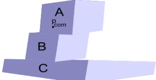
In the traditional Blocks World, the problem is easy to solve using linear logic which includes the notion of state. However, in real life one also has to deal with the problem of achieving balance of blocks while putting a block on another block. We have a new version of the Blocks World named as the Balanced Blocks World 2D, in which the desired order of the blocks is also considered in conjunction with the dynamic balance of blocks [45]. In such a problem, while putting down the block A to the block B, the center of mass of block A should lie on the supporting surface of block B (Figure 3.1). However, only placing the center of mass of the latest placed block on the supporting surface of the block tower would not be enough to satisfy the balance of the entire block tower. The combination of the center of mass of the latest placed block and the top block in a tower should also be on the supporting surface of the second top block in the tower. For the entire block tower, there has to be a check for each block in the tower so that the combination of the centers of mass of the blocks above it have to be on its supporting surface. This modification is introduced into the Traditional Blocks World so that the planning mechanism deals not only with the order of the actions to satisfy the desired goal but also dynamical features of the environment.
Figure 3.1: 3D Illustration of Properly Placing Block A onto Block B
3.2.1
Definition and Domain Properties
In this section, a new blocks world domain called Balanced Blocks World 3D will be described in detail. This domain has the same characteristics with the Balanced Blocks World 2D in that it combines dynamical constraints with state
transitions. However, unlike Balanced Blocks World 2D, the constraint domain is composed of set constraints. Since the only contact part of a newly placed block with the top block in a tower is its base, the points of base areas of blocks will form our sets. For the sake of simplicity, the base of every block is assumed to be the same as its top surface. Figure 3.2 illustrates definitions related to these base areas for every block while Table 3.5 defines concepts and abbreviations in this figure.
Figure 3.2: Concepts in Blocks World 3D
pCOM i center of mass point of Object i at Frame i
mi mass of Object i
Si set of all points in Object i at Frame i
Table 3.5: Abbreviation and Meanings in Blocks World 3D
Each object has its own set and a reference frame called Fi such that its center
of mass is located at the origin. In order to relate the locations of objects to each other, it is necessary that their positions and orientations are represented in the World Frame W . Therefore, we need to rotate and translate all the points of an object from its own frame to the World Frame W . Table 3.6 definitions are needed for that purpose.
We now need to relate these definitions to each other. Equation 3.1 associates the coordinates of the center of mass point of an object with the World Frame W by rotating and translating the center of mass point of an object from its current frame to the World Frame W .
pi an arbitrary point of Object i expressed in Frame i 0
pi an arbitrary point of Object i expressed in the World Frame W 0
Si set of all points of Object i expressed in the World Frame W 0
iR rotation matrix from Frame i to the World Frame W 0
it translation from Frame i to the World Frame W
Table 3.6: Definitions in Blocks World 3D
0
pCOM i= {0
iR pCOM i+ 0
it} (3.1)
Equation 3.2 can be used to transform all points of an object from the current frame to the World Frame W .
0 Si = { 0 iR pi+ 0 it | pi ∈ Si} (3.2)
3.2.2
Constraints
In order to ensure that the tower remains balanced, we should not only check that the new block itself remains in balance, but also make sure that the placement does not disturb existing blocks on the tower. To this end, we recursively compute the center of mass of connected groups of blocks from top to bottom and ensure that all combined centers of mass lie on support surfaces. Thus, the following constraints have to be satisfied to ensure that the towers balanced. We assume that we have k number of objects.
The first constraint is that the center of mass point of the block that is placed on the top block has to be on the support surface of the top block. In set theory, this constraint will be expressed in a way that the center of mass point of the newly placed block has to be the member of the set of all points of the top block in the tower provided that both are on the World Frame W . It is modelled in Equation 3.3.
0
pCOM k ∈ 0
Sk−1 (3.3)
The other constraint is that all the combined center of mass of the connected groups of blocks from top to bottom has to lie on support surfaces. Assume that we have k − 1 number of blocks and we would like to place another block on top of them. In such a condition, we should start to observe that the combination of the center of mass point of the top two blocks should be the member of the set of the top third block. This condition check will continue until reaching the bottom block as an support surface. This constraint is given in Equation 3.4.
i X j=0 mk−j 0 pCOM k−j mk−j pCOM k∈0
Sk−i−1 where i > 0 and i < k − 1 (3.4)
3.2.3
Term Language
So far, we have described the definition and properties of our application domain, relations between these definitions and constraints on this domain. However, all these explanations have to be encoded in a way that they can be used in a logical system. Hence, the term language of our domain will be defined using BNF notation. It will subsequently form the main part of the constrained domain for linear logic.
Set: si | Rotate(Set, Angle) | Translate(Set, Point) |
toSet(Point)
Point: Point Def(Coordinate, Coordinate) | Scale(Point, Point, Mass, Mass) Mass: mi
Coordinate: x | 0 Angle: y
Constraint: Set⊃ Set
In Table 3.7, BNF notations for Blocks World 3D are defined. Here, con-straints consist of only Sets. Since we would like to find whether the center of mass point is the member of a set, the toSet predicate is employed to transform an arbitrary point to the set which will include only one element. In order to rotate and translate the set from its own frame to the World Frame, the Rotate and Translate predicates are used respectively. The Scale predicate calculates the mass balance point between two points. The usage of this encoding will be found in Chapter 4.
Intuitionistic Linear Logic
4.1
Introduction and Motivation
Linear Logic was discovered by J.Y. Girard in 1987 and published in his famous paper [16]. In the abstract of this paper, he states that “completely new approach to the whole area between constructive logics and computer science is initiated”. The fundamental idea under Linear Logic is to control the use of resources.
In Chapter 2, we clarified the difference between Intuitionistic and Classical Logics. One of the important features for Intuitionistic Logic over Classical Logic was the isomorphism between proofs and programs. This has the benefit that each proof in intuitionistic logic directly corresponds to a program. Therefore, a specific domain problem such as robotic planning problem would be possible to solve only searching a proof by using proof search procedures on the application domain that is encoded in logical form. Since we deal with the planning problems, intuitionism will fit for our purpose. The materials in this chapter have been inspired from the Pfenning’s notes about Intuitionistic Linear Logic [36].
In Chapter 3, while describing about the frame problem, we noted that we needed to introduce the notion of state. We have already described the notion of judgement and proposition in Chapter 2. However, this two forms of judgement
is not sufficient to explain logical reasoning from assumptions. Therefore, we need to introduce new primitive notions such as linear hypothetical judgement and linear hypothetical proof. The general form of linear hypothetical judgement can be written as
A1 true, ..., Antrue ⇒ C true.
The meaning of this judgement is that we can prove C from assumptions A1, ..., An, using every assumption exactly once. We say that the left side of the
entailment part is the consumable resources, where the right side is the goal to be achieved. Since the notion of state concept is introduced using such a judgement, the planning problems which are reduced into the state transition problem could be solved by the logical viewpoint.
The judgement above allows only linear hypothesis. Hence, we have no chance to encode ordinary intuitionistic logic to our system. Furthermore, we mostly need some assumptions that will be used everytime, called non-consumable re-sources. Therefore, we need to make a distinction between consumable and non-consumable resources in our representation. Generally, the ∆ letter is used to range over a collection of linear assumptions while the Γ is used to range over a collection of assumptions that are used arbitrarily many times. These letters correspond to a unique context where the ∆ and the Γ letters form the restricted and unrestricted context respectively. For all these definitions, our judgement will be in a form such that:
Γ; ∆ ⇒ A true.
The combination of linearity and intuitionism will allow us to use both the con-sumable resources and proofs-as-programs property. This combination is named as Intuitionistic Linear Logic in literature. The proof theory and the connectives of this logic will be mentioned in later sections.
One has to bear in mind that linear assumptions are viewed as resources and conclusions are viewed as the products by spending the given resources.
Therefore, two of three structural rules, contraction and weakening, of traditional logics are absolutely rejected. The contraction states that a conclusion which follows from two same assumptions can be derived from just one assumption.
Γ; A, A ⇒ B
Γ; A ⇒ B Contraction
The weakening expresses that if a conclusion follows from some assumptions then that conclusion can also be derived after increasing the number of these assumptions.
Γ; A ⇒ B
Γ; A, C ⇒ B W eakening
The only structural rule that intuitionistic linear logic preserve is the exchange which states that the order of the assumptions in derivation does not matter.
Γ; A, C ⇒ B
Γ; C, A ⇒ B Exchange
4.2
Linear Connectives with an Example
In this section, we give an introduction to the linear connectives and an example in order to provide the reader with an initial familiarisation for their meanings and usage. He can also find the formal declarations of these connectives in the next section. Before that, a fundamental formula will be mentioned firstly.
A ⇒ A is the first rule which is derived from the nature of linear hypothetical judgement itself. It means that the resource A is spent to give a product of A.
Now it is time to give an initial information about the linear connectives. One of the most notable feature about the intuitionistic linear logic is that it has two
forms of conjunction (⊗ and &) and two forms of truth (> and 1). On the other hand, there is only one connective for implication (−◦), one form of falsehood (0) and one for disjunction (⊕). There are also various types of linear connectives other than these ones in the literature, however all of the connectives that are mentioned above are utilized for providing intuitionistic purposes while the others satisfy the classical objectives. (e.g. multiplicative disjunction connective (P) and
bottom connective(⊥))
• Linear Implication (−◦):
A −◦ B means that B can be produced by consuming an A. • Simultaneous Conjunction (⊗):
If both A and B are true in the same state then we can write A ⊗ B. A ⊗ B means that our resources can produce both A and B simultaneously. • Alternative Conjunction (&):
A & B means that our resources can make A or B available, but not both simultaneously. This is called internal choice. For instance, if we have one dollar and the price of a coffee and a tea is one dollar, then, we have to make a choice to buy a coffee or tea. Our resource, one dollar, can only produce one of them.
• Disjunction (⊕):
A ⊕ B means that our resources can make either A or B available, but you do not know which one is produced. This is called external choice. For example, if we have one dollar and we would like to buy a coffee or a tea from vending machine and this machine gives us one of them randomly, then A ⊕ B shall be used.
• Unit (1):
The goal 1 can always be produced from the resource of nothing. This is the identity for simultaneous conjunction. (A ⊗ 1 ≡ A)
The goal > can always be achieved regardless of which resource we have. It always consumes all of the resources. > is the identity for alternative conjunction. (A & > ≡ A)
• Impossibility (0):
The 0 is the identity for the disjunction. It corresponds to the impossible resource, so that external choice of 0 and A is always A. (A ⊕ 0 ≡ A) • “Of Course” Modality (!):
The ! is a way to connect the unrestricted hypothesis with restricted ones. It will be described in next section clearly.
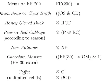
Using these new linear connectives, we can now define an example domain and encode this domain to intensify the meanings of these connectives. The French Restaurant example is one of the famous examples and makes the reader to understand the matter easily.
Menu A: FF 200 FF(200) −◦ Onion Soup or Clear Broth ((OS & CB)
Honey Glazed Duck ⊗ HGD Peas or Red Cabbage ⊗ (P ⊕ RC) (according to season)
New Potatoes ⊗ NP
Chocolate Mousse ((FF(30) −◦ CM) & 1) (FF 30 extra)
Coffee ⊗ C (unlimited refills) ⊗ (!C))
Table 4.1: French Restaurant Menu and Corresponded Linear Logic Encoding
In Table 4.1, note that the alternative conjunction(&) is used when a customer can determine his own meal. However, the disjunction(⊕) is used when a meal
varies according to season. Also he has to pay extra 30 French Francs to eat chocolate mousse or he can choose nothing (1) to eat.
4.3
Proof Theory
Developing linear logic in the form of natural deduction, is highly economical, in that we only need one basic judgement (A true) and two judgement forms (linear and unrestricted hypothetical judgements) to explain the meaning of all connectives we have encountered so far. However, it is not well-suited for proof search, because it involves both forward and backward reasoning.
In Chapter 2, we have mentioned that sequent calculus is the best mechanism to do proof search because of its nature of backward reasoning. In this section, we develop a sequent calculus rather than natural deduction as a calculus of proof search for Intuitionistic Linear Logic.
We now summarize the rules of Intuitionistic Linear Logic. The logic we consider here comprises the following logical operators.
Propositions A := P Atoms
| A1 −◦ A2 | A1⊗ A2 | 1 Multiplicatives
| A1& A2 | > | A1 ⊕ A2 | 0 Additives
| ∀x.A | ∃x.A Quantifiers | A ⊃ B | !A Exponentials
4.3.1
Sequent Calculus
Based on the notion of linear hypothetical judgment, we now introduce the various connectives of Intuitionistic Linear Logic using sequent calculus. Before giving details of linear connectives, we firstly describe two rules. One of them called init explicitly states a connection between resources and goals and the other one called copy relates the unrestricted context and restricted context. Most of the
information in this section is borrowed from Pfenning’s notes about Intuitionistic Linear Logic [36].
Init. It is the basic sequent that means with resource A, we can achieve goal A
Γ; A ⇒ A init.
Copy. It creates a resource from the unrestricted context and copies it into the restricted context
Γ, A; ∆, A ⇒ A
Γ, A; ∆ ⇒ A copy.
The remaining rules are divided into right and left rules. Each linear connec-tive has own left and right rules.
Simultaneous Conjunction. Assume we have some resources and we want to achieve goals A and B simultaneously, written as A ⊗ B (A tensor B). We need to split our resources into ∆1 and ∆2 and show that with resources ∆1 we
can achieve A and with ∆2 we can achieve B
Γ; ∆1 ⇒ A Γ; ∆2 ⇒ B
Γ; ∆1, ∆2 ⇒ A ⊗ B
⊗R
Here, the important part is that the splitting of resources, from bottom to top, is a non-deterministic operation.
The left rule captures that if we achieve goal C using simultaneously occurring resources A and B, then we could achieve same goal C from same resources A and B
Γ; ∆, A, B ⇒ C
Alternative Conjunction. We write A & B if we can goals A and B with the current resources, but only alternatively. The right rule for the alternative conjunction asserts that if we achieve goal A & B from resources ∆, then we could achieve goal A or alternatively B from same resource ∆
Γ; ∆ ⇒ A Γ; ∆ ⇒ B Γ; ∆ ⇒ A & B &R.
The right rule for alternative conjunction appears to duplicate the resources. However, this is an illusion: since we will actually have to make a choice between A and B, we will only need one copy of the resources.
If we achieve goal C from resources A & B, we could achieve the same goal C, either from A or B but alternatively. Therefore we need two left rules for that purpose:
Γ; ∆, A ⇒ C
Γ; ∆, A & B ⇒ C &L1
Γ; ∆, B ⇒ C
Γ; ∆, A & B ⇒ C &L2.
Linear Implication. The linear implication incorporates the linear hypo-thetical judgement within level of propositions. A −◦ B (pronounced A linearly implies B) is used for the goal of achieving B with resource A. Formally, if we have resource ∆ to achieve goal A −◦ B, then we can achieve goal B from resources ∆ and A
Γ; ∆, A ⇒ B
Γ; ∆ ⇒ A −◦ B −◦ R.
The left rule for linear implication needs splitting resources as in the right rule of simultaneous conjunction. Assume that if we have resources ∆ and A −◦ B to achieve goal C, then we need to divide our resource ∆ into two parts such as ∆1
and ∆2 to achieve goal A from resource ∆1 and to achieve goal C from resources
Γ; ∆1 ⇒ A Γ; ∆2, B ⇒ C
Γ; ∆1, ∆2, A −◦ B ⇒ C
−◦ L .
Unit. The trivial goal which requires no resources is written as 1
Γ; . ⇒ 1 1R.
The left rule asserts that if we have resource 1 to achieve goal C, then we could achieve the same goal C without the resource 1
Γ; ∆ ⇒ C Γ; ∆, 1 ⇒ C 1L.
Top. The goal which consumes all resources is written as >
Γ; ∆ ⇒ > >R.
It is the unit of alternative conjunction and there is no elimination for the >. Disjunction. The disjunction A ⊕ B (called as external choice) is character-ized by two introduction rules
Γ; ∆ ⇒ A
Γ; ∆ ⇒ A ⊕ B ⊕R1
Γ; ∆ ⇒ B
Γ; ∆ ⇒ A ⊕ B ⊕R2.
The left rule of disjunction asserts that if we have resources A ⊕ B and ∆ to achieve goal C, then we could achieve the same goal C from A and ∆ or B and ∆
Γ; ∆, A ⇒ C Γ; ∆, B ⇒ C Γ; ∆, A ⊕ B ⇒ C ⊕L.