Journal of Physics B: Atomic, Molecular and Optical Physics
PAPER
Non-Markovian dynamics in ultracold Rydberg
aggregates
To cite this article: M Genkin et al 2016 J. Phys. B: At. Mol. Opt. Phys. 49 134001
View the article online for updates and enhancements.
Related content
Mølmer–Sørensen entangling gate for cavity QED systems
Hiroki Takahashi, Pedro Nevado and Matthias Keller
-Efficient real-time path integrals for non-Markovian spin-boson models A Strathearn, B W Lovett and P Kirton
-Non-Markovianity in the optimal control of an open quantum system described by hierarchical equations of motion E Mangaud, R Puthumpally-Joseph, D Sugny et al.
-Recent citations
Trapped-ion quantum simulation of excitation transport: Disordered, noisy, and long-range connected quantum networks N. Trautmann and P. Hauke
-Engineering thermal reservoirs for ultracold dipole–dipole-interacting Rydberg atoms
D W Schönleber et al
-Rydberg aggregates S Wüster and J-M Rost
1
Max-Planck-Institute for the Physics of Complex Systems, D-01187 Dresden, Germany
2
Department of Physics, Bilkent University, Ankara 06800, Turkey E-mail:[email protected]
Received 25 February 2016, revised 21 April 2016 Accepted for publication 29 April 2016
Published 31 May 2016 Abstract
We propose a setup of an open quantum system in which the environment can be tuned such that either Markovian or non-Markovian system dynamics can be achieved. The implementation uses ultracold Rydberg atoms, relying on their strong long-range interactions. Our suggestion extends the features available for quantum simulators of molecular systems employing Rydberg aggregates and presents a new test bench for fundamental studies of the classification of system– environment interactions and the resulting system dynamics in open quantum systems. Keywords: Rydberg aggregates, dipole–dipole interactions, electromagnetically induced transparency, open quantum systems, non-Markovian dynamics
(Some figures may appear in colour only in the online journal) 1. Introduction
The formalism of open quantum systems, i.e., quantum sys-tems interacting with an environment, is a widely used con-cept in many areas of physics. Its backbone is the separation of a large quantum system into a small system of interest and an environment, encapsulating all other degrees of freedom present in the full system. Sometimes, such an approach makes it possible to derive a tractable and physically mean-ingful equation of motion for the small system, rather than propagating the full system in time. This concept[1, 2] has become a common tool in atomic, molecular, and condensed matter systems, and also finds applications in nuclear [3,4] and particle[5,6] physics. It is further crucially important in thefield of quantum information and computation, making it possible to assess the role of decoherence in quantum infor-mation protocols[7].
In many physical systems, the environment consists of a large number of degrees of freedom at finite temperature. Often, such an environment exhibits a back-action onto the system, which depends on previous system dynamics. In open quantum system terms, this memory of the environment is related to the concept of(non-)Markovianity.
From a practical point of view, a memoryless (Marko-vian) environment enables one to derive simple equations of motion, such as the Lindblad form [8], that allow for an
efficient numerical solution of the dynamics restricted to the small system space. For strongly coupled environments with memory, typically sophisticated and numerically expensive methods are required. From this point of view it would be advantageous to possess so called quantum simulators[9,10] that can capture such non-Markovian dynamics. Over the last years, several setups have been suggested with which such non-Markovian quantum simulators could be realized [11–20].
In the present work, we propose an experimentally fea-sible setup where Markovian and non-Markovian dynamics can be studied in a controlled fashion using ultracold Rydberg atoms. The idea relies on the combination of two achieve-ments, which have been reached separately in two recent experiments: coherent oscillations of a Rydberg dimer due to resonant dipole–dipole interactions [21] and imaging of a Rydberg excitation by destroying the resonance condition of electromagnetically induced transparency (EIT) for a back-ground gas through van der Waals interactions [22, 23]. Interfacing a coupled Rydberg dimer with an optically driven background gas atom provides, on the one hand, a test bench to study the Markovian to non-Markovian transition, and on the other hand it might be useful in view of recent proposals to use Rydberg ensembles as quantum simulators for open quantum systems[24–26].
We first describe the setup in detail in section 2, and present our numerical results with experimentally accessible parameters in section 3. In section 4, the results are sum-marized and their implications for future work are discussed. We set ÿ=1 throughout the manuscript.
2. Setup
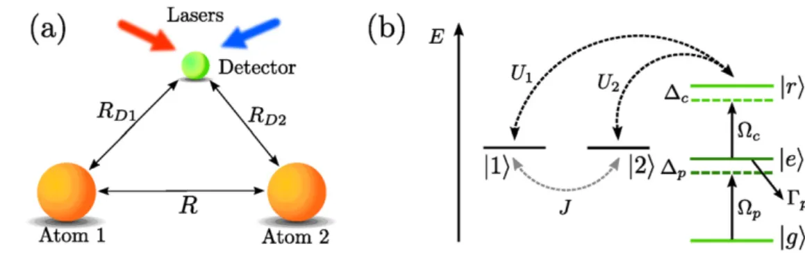
The basic setup and the relevant states are sketched in figure1. We consider two Rydberg atoms(Rydberg dimer’) in states ∣añ = ∣nℓ and ∣ñ bñ =∣n¢ ¢ñℓ respectively, withν, ν’ denoting the(large) principal quantum numbers and ℓ, ¢ℓ the angular momentum quantum numbers. The state con figura-tion is chosen such that coherent Rabi oscillafigura-tions due to resonant dipole–dipole interactions [21] are enabled between the pair states ∣1ñ =∣a b, ñand ∣2ñ =∣b a, ñ. The essential dynamics for the pair states specified below is thus captured in a two-state picture with the Hamiltonian
(∣ ∣ ∣ ∣) ( )
= ñá + ñá
HS J 2 1 1 2 . 1
Here, J denotes the resonant dipole–dipole matrix element given by J=C R3 3, where C3 is a state-dependent
interac-tion coefficient and R the interatomic separation of the dimer (see figure1(a)). The dimer constitutes our system S. We now bring a third, laser-driven atom into the vicinity of the dimer. This driven atom constitutes our environment and is from now on referred to as the detector[25]. The laser field (probe field) couples the ground state ∣ ñg of the detector atom to some intermediate level ∣ ñe , which in turn is coupled to a Rydberg state ∣ ñr by a second laserfield (control field). In the rotating wave approximation, the detector is described by the Hamiltonian ∣ ∣ ∣ ∣ ∣ ∣ ( )∣ ∣ ( ) = W ñá + W ñá + - D ñá - D + D ñá ⎛ ⎝ ⎜ ⎞⎠⎟ H e g r e e e r r 2 2 h.c. , 2 D p c p p c
where Ωp, Ωc denote the Rabi frequencies and Δp, Δc the
detunings of the probe- and coupling fields. As Rydberg states have a very long (though finite) lifetime [27,28], we
neglect the spontaneous decay of the state ∣ ñr in our scheme. The intermediate state ∣ ñe , however, is chosen to undergo radiative decay, which takes place on the time scale of the dynamics of the system. In order to account for this effect, we model the spontaneous decay with rateΓpfrom this level by
the Lindblad operator
∣ ∣ ( )
= G ñá
L p g e . 3
In the absence of interactions between the dimer(system) and the detector(environment), the dimer dynamics is simply governed by the unitary von-Neumann equation
˙ [ ] ( )
rS= - Hi S,rS 4
and the dynamics of the detector (environment) by a master equation in Lindblad form
˙ [ ] ( † † †) ( )
r = -i H ,r - 1 r L L+L Lr - Lr L
2 2 . 5
D D D D D D
Here, ρS and ρD are the density operators of system and
detector, respectively. The system–environment coupling emerges due to strong van-der-Waals-type interactions between the Rydberg state of the detector with the Rydberg states of the dimer.
Our exploitation of a single three-level atom as an ‘environment’ may seem unusual, given the more typical situation where the environment is characterized by a parti-cularly large number of quantum states. It makes sense though, since the Lindblad treatment of spontaneous decay (3) embodies the coupling of this atom to the radiation field, which even if in the vacuum has a large number of quantum states available.
We now specify the states of the Rydberg atoms of our proposal. As in[25] we take the dimer states to be ∣1ñ =∣psñ and ∣2ñ =∣spñ, with ∣pñ = ∣43pñ and ∣sñ = ∣43sñ of 87Rb. These dimer states are coupled via dipole–dipole interaction, which results in a Hamiltonian of the form of equation (1), withC 23 p=1619 MHz mm 3. For the states of the detector we take ∣rñ = ∣38 , ∣sñ eñ =∣5pñand ∣gñ =∣5sñ[23]. Then, the interactions between the dimer states ∣ ñ1 and ∣ ñ2 and the Figure 1.Sketch of the setup.(a) Atoms 1 and 2 form the Rydberg dimer with interatomic separation R, and the laser-driven detector atom placed in their vicinity. The distances of the detector to the dimer atoms are denoted by RD1and RD2, respectively.(b) Level sketch of the
setup. The dimer states∣ ñ1 and ∣ ñ2 are coupled to each other via resonant dipole–dipole interaction with strength J and interact with the Rydberg level∣ ñr of the detector atom via the interactions U1, U2. The ground state∣ ñg of the detector is coupled to the state ∣ ñe by the probe
field with Rabi frequency Wpand detuningΔp, and the state∣ ñe to the Rydberg level ∣ ñr by the controlfield (Ωc,Δc). Γpis the spontaneous
decay rate of the level∣ ñe .
2
separation of the detector from atom 1 and atom 2 of the dimer. The system–environment interactions (6) conserve the system population. Note that our proposal does not rely on the specific states chosen, but on the state-dependence of interactions between dimer and detector, which, in principle, can also be achieved with different choices.
The system–environment interaction Hamiltonian can then be written as
∣ ∣ ∣ ∣ ∣ ∣ ∣ ∣ ( )
= ñá Ä ñá + ñá Ä ñá
HSD U1 1 1 r r U2 2 2 r r 7
and the master equation encapsulating the system, the environment and their interaction reads as
˙ [ ] ( † † †) ( )
r= -i H,r - 1 rK K+K Kr- K Kr
2 2 . 8
Here,ρ is the full density operator, H the full Hamiltonian ( )
= Ä + Ä +
H HS D S HD H ,SD 9
the unity operator in a given Hilbert space and K is the extension of the Lindblad operator L in the full Hilbert space,
= Ä
K S L with L given in equation(3).
3. Numerical results
In this section, we show illustrative calculations that demonstrate that, despite its simplicity, the environment provided by the detector atom is highly tunable, and in particular that the time evolution of the dimer can be tuned from Markovian to various degrees of non-Markovian dynamics. Over the last few years, a suitable measure to quantify non-Markovianity in an open quantum system has been actively pursued and debated(see e.g. [29–48]), as well as used to gain insight into the dynamics of physical systems [16,49–51]. In what follows, we adopt the measure related to the informationflow from the environment to the system [31]. By this definition, the dynamics is non-Markovian whenever the trace distance between two initial density operators of the system increases at some point during their time propagation. The trace distance between two density matrices P, Q is defined as
( )= ∣ - ∣ ( )
D P Q, 1 P Q
2Tr , 10
with ∣ ∣A = A A† . For a two-level system (∣1 , 2ñ ∣ ñ), this expression simplifies to [30]
( )= ( - ) +∣ - ∣ ( ) D P Q, P11 Q112 P21 Q212. 11 ( ( ) ( )) ( ) =
ò
s s> dt t P, 0 ,Q 0 . 13 P Q, 0Note that to obtain an actual measure, maximization over all pairs (P(0), Q(0)) has to be performed in equation (13) [30, 31]. In the following, we take initial states
( ) ∣ ∣ ∣ ∣
r1 0 = ñá Ä ñá1 1 g g andr2( )0 = ñá Ä ñá∣2 2∣ ∣g g∣, which can be easily prepared(and probed) experimentally and have numerically shown to yield large values r r1, 2 [52]. The corresponding system states rS,i( )0 =TrDri( ) (0 , i=1, 2) have maximal initial trace distance D(rS,1( )0 ,rS,2( ))0 =1. We propagate both states in time according to equation (8) and thereupon obtain the trace distance DSand the rateσSin
the subsystem of interest (dimer) by tracing out the environment first and subsequently applying the definitions (10) and (12).
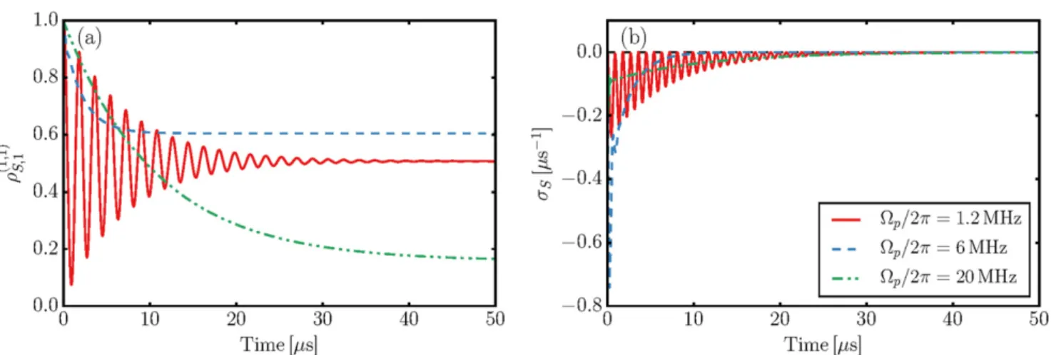
Before discussing non-Markovianity we illustrate how the dimer dynamics depends on the properties of the environment constituted by the detector atom, and how these properties can be tuned. In figure 2(a) we show different dimer dynamics arising for different Rabi frequencies Ωp of
the probefield driving the detector atom, indicating that both dephasing strength and steady-state value of the dimer dynamics can be easily controlled via the parameters of lasers acting on the detector atom.
The different strengths of dephasing can be understood on grounds of the strong asymmetry in the interactions
U1 U2. In this way, the environment can distinguish whe-ther the system is in state ∣ ñ1 or ∣ ñ2 and acts as a measurement device, causing dephasing and decoherence in the system [25]. Consider the case when the laser fields are applied resonantly, Δp=Δc=0. The detector is then tuned to the
condition of EIT [53], giving rise to a so called dark state which has no contribution from state ∣ ñe . If the dimer is in the state ∣ ñ2 , the detector remains in the dark state since the interaction U2 is negligible by design of the experiment.
However, if the dimer is in the state ∣ ñ1 , the strong interaction U1 shifts the Rydberg level of the detector ∣ ñr out of
reso-nance, disturbing the EIT condition, which yields a non-zero population of the state ∣ ñe . This state then decays with the rate Γp, and the emitted photons provide a potential observer with
information about the state of the dimer. The stronger the drivingΩp, the more photons will be scattered by the detector
atom, allowing to infer the state of the dimer more quickly, and thereby dephasing the dimer dynamics more quickly.
However, as depicted in figure 2(b), various dimer dynamics with vastly different dephasing time scales and steady-state values can still be purely Markovian according to equation(13). This cautions one that looking at the population
dynamics alone can be misleading when trying to estimate the Markovianity of the dynamics.
We now demonstrate the tunability of our setup. By modifying the interatomic distances as well as the laser parameters, we can switch the dimer dynamics from Marko-vian to non-MarkoMarko-vian, as shown in figure 3. Now, strong oscillations withσS>0 can be seen in figure3(b), leading to
a clearly nonzero r r1, 2»2.7quantifying non-Markovianity. In the chosen configuration, the non-Markovianity of the system dynamics is not only reflected in the trace distance change rate σS, but can also be seen in the population
dynamicsfigure3(a) which displays a clear revival at ≈1 μs of the damped population oscillations.
It has to be noted, though, that visible non-Markovian features in the population dynamics are not necessarily pre-sent even if the system dynamics is non-Markovian. Indeed,
in figure 4 we show another example of non-Markovian system dynamics, in which the clearly positive contributions σS>0 in panel (b) lead to a nonzero r r1, 2»0.2while the population dynamics displayed in panel (a) does not exhibit noticeable revivals or other features often associated with non-Markovian dynamics. Comparing the figures obtained from equation(13), we see that r r1, 2and thus the degree of non-Markovianity is significantly larger in figure 3 than in figure 4, explaining the lack of non-Markovian features observed in the population dynamics in figure 4. Upon decreasing the rate of dissipation in the environment (spon-taneous decay rateΓp), however, even in this setting revivals
become visible.
In summary, to observe non-Markovianity in the system dynamics we have found that one needs several ingredients: (i) long detector equilibration time and intrinsic dynamics in Figure 2.Dynamics of the system(dimer) for three different values of the Rabi frequency Ωp. Panel(a) shows the population of the state ∣ ñ1 for
the initial stateρ1(0), and panel (b) the trace distance change rate σSbetweenρS,1(t) and ρS,2(t) in the system, if system plus environment are
prepared inρ1(0) and ρ2(0), respectively (see main text). The parameters are Γp/2π=6.1 MHz, J/2π=0.28 MHz, Ωc/2π=20 MHz, U1/
2π=−26.4 MHz and U2/2π=−0.37 MHz, corresponding to the interatomic distances R=18 μm, R1D=2.5 μm and R2D=15.5 μm. The
detuningsΔp,Δcare set to zero. The Rabi frequencies areΩp/2π=1.2 MHz (red solid curve), Ωp/2π=6 MHz (blue dashed curve) and Ωp/
2π=20 MHz (green dashed–dotted curve). As evident from the time evolution of σS, the three sets correspond to completely Markovian system
dynamics according to the definition equation (13), although the population dynamics in the system shows very different equilibration time scales as well as steady-state values.
Figure 3.Same as infigure2but using the parametersJ 2p =3.16 MHz,Wp 2p= Wc 2p=30 MHz, U1/2π=−36.9 MHz, and U2/
2π=−0.8 MHz, corresponding to the interatomic distances R=8 μm, R1D=2.3 μm and R2D=8.3μm. The detunings are
p p
Dc 2 = -Dp 2 =50 MHz. As evident from the time evolution ofσS, the system dynamics is non-Markovian(r r1, 2»2.7), also
reflected in the population revival at ≈1 μs seen in panel (a).
4
the detector atom. Long detector equilibration time can be achieved by e.g. reducing the radiative decay rateΓp(which
is, however, experimentally impractical) or by introducing a large detuningΔpof the intermediate state while at the same
time keeping the two-photon resonance condition Δp+Δc∼0. (ii)Comparability of time scales of aggregate
and detector dynamics. This can be most easily attained by tuning the aggregate coupling J, as the detector time scale results from a complex interplay of laser parameters, radiative decay and interactions. (iii)Correlation between aggregate dynamics and photon emission from the detector atom, i.e., ability to deduce the state of the aggregate by measuring the photons emitted by the detector atom. Though this condition is not fully separable from the previous one(ii), it can be met by ensuring a strong interaction U1between aggregate atom 1
and detector atom and a strong asymmetryU1U2between the interactions U1and U2of the two aggregate atoms with
the detector atom. Whereas thefirst condition (i) guarantees the presence of environment memory,(ii) and (iii) guarantee the visibility of the environment dynamics in the system dynamics. This can be seen infigures3 and4: to reduce the degree of non-Markovianity in figure 4 as compared to figure3, we reduced the detuning ∣Dp∣, the interaction U1and
the aggregate coupling J. Reducing the detuning ∣Dp∣ decreases the equilibration time of the detector dynamics, decreasing the interaction U1reduces the correlation between
aggregate and detector, and reducing the aggregate coupling J decreases the visibility of the back-action induced by the detector dynamics.
4. Discussion and summary
The presented setup provides a test bench to study con-trollable non-Markovianity in open quantum systems. We have shown that both Markovian as well as non-Markovian system dynamics can be achieved by the driven-dissipative environment provided by the detector atom. Besides, our
analysis reveals that (non-)Markovianity of the system (dimer) dynamics cannot be easily inferred from population dynamics alone, but rather a measure relying on the infor-mation provided by the full density matrix of the system has to be employed.
Our proposal represents afirst step towards a non-Mar-kovian quantum simulator harnessing ultracold Rydberg atoms and should be accessible by state-of-the-art exper-imental setups. In addition to using the environment as a measurement device for the dimer dynamics[22,23,25], in our setup the single detector atom operates as gateway to the environment of electromagnetic field modes implicitly responsible for its spontaneous decay. The system dynamics can be extracted by different means[21].
Having shown the variety of Markovian/non-Markovian dynamics as well as dephasing time scales and steady-state values of the system in the case of a simple setup employing a single detector atom, we expect even richer tunability of the dynamics in the case of many detector atoms. This might open up new prospects for using Rydberg aggregates as quantum simulators with a controlled environment.
Acknowledgments
We thank Shannon Whitlock and Kimmo Luoma for helpful discussions.
References
[1] May V and Kühn O 2011 Charge and Energy Transfer Dynamics in Molecular Systems(New York: Wiley) [2] Breuer H P and Petruccione F 2002 The Theory of Open
Quantum Systems(Oxford: Oxford University Press) [3] Antonenko N V, Ivanova S P, Jolos R V and Scheid W 1994
Phys. G: Nucl. Part. Phys.20 1447
[4] Diaz-Torres A, Hinde D J, Dasgupta M, Milburn G J and Tostevin J A 2008 Phys. Rev. C78 064604
Figure 4.Same as infigure2but using the parameters J/2π=1.89 MHz,Wp2p= Wc 2p=30 MHz, U1/2π=−4 MHz, and U2/
2π=−0.11 MHz, corresponding to the interatomic distances R=9.5 μm, R1D=4 μm and R2D=10.3 μm. The detunings are
p p
Dc 2 = -Dp 2 =20 MHz. As can be seen from the time evolution ofσS, the system dynamics is non-Markovian(r r1, 2»0.2),
[5] Caban P, Rembielinski J, Smolinski K A and Walczak Z 2005 Phys. Rev. A72 032106
[6] Bertlmann R A, Grimus W and Hiesmayr B C 2006 Phys. Rev. A73 054101
[7] Nielsen M A and Chuang I L 2000 Quantum Computation and Quantum Information(Cambridge: Cambridge University Press)
[8] Lindblad G 1976 Commun. Math. Phys.48 119 [9] Feynman R P 1982 Int. J. Theor. Phys.21 467 [10] Feynman R P 1986 Found. Phys.16 507
[11] Georgescu I M, Ashhab S and Nori F 2014 Rev. Mod. Phys. 86 153
[12] Herrera F and Krems R V 2011 Phys. Rev. A84 051401 [13] Mostame S, Rebentrost P, Eisfeld A, Kerman A J,
Tsomokos D I and Aspuru-Guzik A 2012 New J. Phys.14 105013
[14] Eisfeld A and Briggs J S 2012 Phys. Rev. E85 046118 [15] Stojanović V M, Shi T, Bruder C and Cirac J I 2012 Phys. Rev.
Lett.109 250501
[16] Chiuri A, Greganti C, Mazzola L, Paternostro M and Mataloni P 2012 Sci. Rep.2 968
[17] Mei F, Stojanović V M, Siddiqi I and Tian L 2013 Phys. Rev. B88 224502
[18] Jin J, Giovannetti V, Fazio R, Sciarrino F, Mataloni P, Crespi A and Osellame R 2015 Phys. Rev. A91 012122 [19] Man Z-X, Xia Y-J and Lo Franco R 2015 Sci. Rep. 5 13843 [20] Brito F and Werlang T 2015 New J. Phys.17 072001 [21] Ravets S, Labuhn H, Barredo D, Béguin L, Lahaye T and
Browaeys A 2014 Nat. Phys.10 914
[22] Günter G, de Saint-Vincent M R, Schempp H, Hofmann C S, Whitlock S and Weidemüller M 2012 Phys. Rev. Lett.108 013002
[23] Günter G, Schempp H, de Saint-Vincent M R, Gavryusev V, Helmrich S, Hofmann C S, Whitlock S and Weidemüller M 2013 Science342 954
[24] Hague J P and MacCormick C 2012 Phys. Rev. Lett.109 223001
[25] Schönleber D W, Eisfeld A, Genkin M, Whitlock S and Wüster S 2015 Phys. Rev. Lett.114 123005
[26] Schempp H, Günter G, Wüster S, Weidemüller M and Whitlock S 2015 Phys. Rev. Lett.115 093002
[27] Gallagher T 2005 Rydberg Atoms, Cambridge Monographs on Atomic, Molecular and Chemical Physics(Cambridge: Cambridge University Press)
[28] Beterov I I, Ryabtsev I I, Tretyakov D B and Entin V M 2009 Phys. Rev. A79 052504
[29] Rivas A, Huelga S F and Plenio M B 2014 Rep. Prog. Phys.77 094001
[30] Breuer H P 2012 J. Phys. B: At. Mol. Opt. Phys.45 154001 [31] Breuer H P, Laine E M and Piilo J 2009 Phys. Rev. Lett.103
210401
[32] Rivas A, Huelga S F and Plenio M B 2010 Phys. Rev. Lett.105 050403
[33] Haikka P, Cresser J D and Maniscalco S 2011 Phys. Rev. A83 012112
[34] Chruscinski D, Kossakowski A and Rivas A 2011 Phys. Rev. A 83 052128
[35] Luo S, Fu S and Song H 2012 Phys. Rev. A86 044101 [36] Haikka P, Goold J, McEndoo S, Plastina F and Maniscalco S
2012 Phys. Rev. A85 060101
[37] Rosario A, Massoni E and Zela F D 2012 J. Phys. B: At. Mol. Opt. Phys.45 095501
[38] Lorenzo S, Plastina F and Paternostro M 2013 Phys. Rev. A88 020102(R)
[39] Smirne A, Mazzola L, Paternostro M and Vacchini B 2013 Phys. Rev. A87 052129
[40] Hall M J W, Cresser J D, Li L and Andersson E 2014 Phys. Rev. A89 042120
[41] Ma T, Chen Y, Chen T, Hedemann S R and Yu T 2014 Phys. Rev. A90 042108
[42] Fanchini F, Karpat G, Cakmak B, Castelano L, Aguilar G, Farias O J, Walborn S, Ribeiro P S and de Oliveira M 2014 Phys. Rev. Lett.112 210402
[43] Chruscinski D and Maniscalco S 2014 Phys. Rev. Lett.112 120404
[44] He Z, Yao C, Wang Q and Zou J 2014 Phys. Rev. A90 042101 [45] Addis C, Bylicka B, Chruscinski D and Maniscalco S 2014
Phys. Rev. A90 042101
[46] Haseli S, Karpat G, Salimi S, Khorashad A S, Fanchini F F, Cakmak B, Aguilar G H, Walborn S P and Ribeiro P H S 2014 Phys. Rev. A90 052118
[47] Hou S C, Liang S L and Yi X X 2015 Phys. Rev. A91 012109
[48] Overbeck V R and Weimer H 2016 Phys. Rev. A93 012106 [49] Liu B H, Li L, Huang Y F, Li C F, Guo G C, Laine E M,
Breuer H P and Piilo J 2011 Nat. Phys.7 931
[50] Tang J S, Li C F, Li Y L, Zou X B, Guo G C, Breuer H P, Laine E M and Piilo J 2012 Eur. Phys. Lett.97 10002 [51] Luoma K, Haikka P and Piilo J 2014 Phys. Rev. A90 054101 [52] Li J-G, Zou J and Shao B 2010 Phys. Rev. A81 062124 [53] Fleischhauer M, Imamoglu A and Marangos J P 2005 Rev.
Mod. Phys.77 633
6