DOĞUŞ UNIVERSITY
INSTITUTE OF SOCIAL SCIENCES
MASTER OF SCIENCE IN FINANCIAL ECONOMICS
CAPITAL ASSET PRICING MODEL AND BANKING SECTOR APPLICATION IN ISTANBUL STOCK EXCHANGE MARKET (1999-2009)
Master Thesis
Musa Gün 200786004
Advisor:
ABSTRACT
Capital Asset Pricing Model and Banking Sector Application in Istanbul Stock Exchange Market
Capital Asset Pricing Model (CAPM) and Arbitrage Pricing Model are two main asset pricing models that explain capital asset pricing and stock returns in financial theory.
The purpose of this study is to search the validity of CAPM, which is also known as the capital market equilibrium model, in our country.
In the application of the research daily closing prices of 11 banks stocks that are traded in Istanbul Stock Exchange Market (ISE) are evaluated over the 1999-2009 period.
There are two main reasons while choosing banking sector in order to test the validity of CAPM;
Banking sector in the ISE is subject to more controls and audits compared to other sectors. Therefore, assets chosen from the banking sector have less possibility of overpricing, under-pricing or manipulation risks over the prices. Thus, probability of reflecting the right prices of the assets is higher for the banking sector assets.
Secondly, changes in the interest rates are immediately reflected in banking sector, since their affairs based on interest rates banks are highly sensitive to interest rate changes. This sensitivity played a crucial role to consider banking sector assets. In the research performed by Copeland, Koller and Murrin (1994) it is observed that beta of banking sector is the most close to the market beta. Thereupon, it is thought that market representation likelihood of banking sector is high.
ÖZET
Finansal Varlık Fiyatlama Modeli ve İstanbul Menkul Kıymetler Borsası Bankacılık Sektörü Uygulaması
Finansal Varlık Fiyatlama Modeli ve Arbitraj Fiyatlama Modeli, finans teorisinde finansal varlıkların fiyatlanması ve bu varlıkların getirilerini açıklamaya yönelik temel fiyatlama modelleri olarak yer almaktadırlar.
Bu çalışmanın amacı sermaye pazarı denge modeli olarak da bilinen Finansal Varlık Fiyatlama Modeli’nin ülkemizde geçerliliğini araştırmaktır.
Araştırma gerçekleştirilirken ülkemizde bankacılık alanında faaliyette bulunan ve sermaye piyasası pazarı olarak bilinen İstanbul Menkul Kıymetler Borsası (IMKB)’nda hisselerinin alım satımı yapılan 11 adet banka hissesinin 1999–2009 dönemindeki günlük hisse kapanış fiyat verileri dikkate alınmıştır.
Finansal Varlık Fiyatlama Modeli’nin geçerliliği test edilirken bankacılık sektörünün tercih edilmesinin iki temel nedeni bulunmaktadır;
Bankacılık sektörü İMKB’de işlem gören diğer sektörlere nispeten daha fazla denetime ve kontrollere tabi olan bir sektör olarak yer almaktadır. Bu nedenle ilgili sektörden seçilen hisse fiyatları üzerinde olası yüksek veya düşük değerlemelerin ve manipülasyonların daha az olması beklenmektedir. Bu da fiyat verilerinin gerçeği yansıtma olasılığını arttırmaktadır.
Bankacılık sektörünün faaliyetlerinin faizlerde meydana gelecek değişiklikleri anında yansıtması, faiz değişikliklerine karşı duyarlılığın yüksek olması bankacılık sektörü verilerinin tercih edilmesinde önemli olmuştur. Copeland, Koller ve Murrin (1994) tarafından yapılan
TABLE of CONTENTS
ABSTRACT... i
ÖZET ... ii
LIST of FIGURES ... v
LIST of TABLES ... vii
LIST of ABBREVIATIONS ... viii
PART 1 INTRODUCTION... 1
PART 2 MAIN CONCEPTS OF RISK ... 4
2.1 Risk and Fundamental Types of Risk ... 4
2.1.1 Systematic Risk... 8
2.1.2 Unsystematic Risk ... 9
2.1.3 Credit or Default Risk... 9
2.1.4 Country Risk ... 10
2.1.5 Foreign-Exchange Risk... 10
2.1.6 Interest Rate Risk... 10
2.1.7 Political Risk... 10
2.1.8 Market Risk... 10
2.2 Measuring Risk for a Single Asset and Portfolio Risk Composed of Two Assets... 12
2.3 Measuring Risk for a Portfolio Composed of “n” Number of Assets ... 17
2.4 Types of Investors under Different Risk Preferences... 20
2.5 Return and Its Calculation ... 26
PART 3 MODERN PORTFOLIO THEORY ... 31
3.1 The Theory and Its Assumptions ... 31
3.1.1 Assumptions of modern portfolio theory... 32
3.2 Efficient Frontier... 33
3.3 Determination of Optimal Portfolio on Efficient Frontier with the Help of Indifference Curves ... 34
4.2 The Capital Market Line (CML) ... 38
4.3 Expected Return and Risk of A Portfolio Consisted of Risk-free and Risky Assets.... 43
4.4 Optimal Portfolio Selection ... 44
PART 5 CAPITAL ASSET PRICING MODEL ... 46
5.1 Assumptions of CAPM... 46
5.2 Derivation of the CAPM... 49
5.3 Security Market Line and Comparison with Capital Market Line ... 53
5.4 Characteristic of the CAPM... 59
5.5 Beta Estimation... 61
5.5.1 Historical Market Betas ... 62
5.5.2 Fundamental Beta ... 64
5.5.3 Accounting Beta ... 64
5.6 Unrealistic Assumptions and Limitations of CAPM ... 66
5.6.1 Consumption... 73
5.6.2 Portfolio Restrictions ... 73
5.6.3 Market Proxy Problem... 75
5.6.4 Size Effect... 76
5.6.5 Value Effect ... 77
5.6.6 Momentum Effect ... 79
5.6.7 Mean Reversion Effect ... 80
5.6.8 Horizon Effects ... 80
PART 6 TESTING CAPM FOR BANKING SECTOR... 82
6.1 Test Methodology and Data... 82
6.2 Calculation of Security Characteristic Line (SCL)... 88
6.3 Security Market Line Regression ... 102
LIST of FIGURES
Figure 2.1 The standard deviation of portfolio return as a function of the number of securities
in the portfolio ... 11
Figure 2.2 Scattered correlation graphs between two variables ... 16
Figure 2.3 Indifference curve... 21
Figure 2.4 Indifference curve of absolutely risk insensitive investor... 23
Figure 2.5 Indifference curve of absolutely risk sensitive investor... 24
Figure 2.6 Indifference curve of risk averse investor ... 25
Figure 2.7 Indifference curve of risk lover investor ... 25
Figure 3.1 Efficient frontier ... 33
Figure 3.2 Determination of optimal portfolio on efficient frontier ... 35
Figure 3.3 Optimal portfolio determination under different risk preferences of investors... 36
Figure 4.1 Capital market line ... 39
Figure 4.2 Expected return calculation of a portfolio on capital market line ... 40
Figure 4.3 Portfolio choice of investors on the capital market line... 42
Figure 4.4 Optimal portfolio selection along CML ... 44
Figure 5.1 Optimal risk portfolio-market portfolio ... 49
Figure 5.2 Graph of Security Market Line ... 54
Figure 5.3 Security market line... 58
Figure 5.4 Capital market line with no risk free rate ... 67
Figure 5.5 Minimum variance frontier without short sales ... 74
Figure 5.6 A minimum-variance frontier with restrictions... 75
Figure 5.7 Stocks grouped by size. ... 76
Figure 5.8 Size effect for a positive slope of SML... 77
Figure 5.9 Mean excess returns against market-beta... 78
Figure 5.10 Momentum in the short run and mean-reversion in the long run... 79
Figure 5.11 The effect of estimation risk and the investment horizon ... 81
Figure 6.3 Excess returns over the risk free rate on the stock and on the market index... 91
Figure 6.4 Risk premium distribution... 95
Figure 6.5 Alpha distribution of stocks and indices ... 97
Figure 6.6 Beta distribution of the regression... 99
Figure 6.7 Residual variances... 100
Figure 6.8 Security market regression line……….102
Figure 6.9 SML regression over annul data………104
LIST of TABLES
Table 2.1 Overall portfolio return... 29
Table 6.1 Risk premiums of stocks and indices... 86
Table 6.2 Beta calculation of risk free asset over different indices... 92
Table 6.3 Alpha distribution of stocks and indices... 94
Table 6.4 Beta comparison ... 98
Table 6.5 Adjusted R Squares... 101
LIST of ABBREVIATIONS
APT : Arbitrage Pricing Theory
B/M : Book/Market Ratio
CAPM : Capital Asset Pricing Model CML : Capital Market Line
ISE : Istanbul Stock Exchange Market
IMKB : İstanbul Menkul Kıymetler Borsası
MPT : Modern Portfolio Theory
MRS : Marginal Rate of Substitution
NYSE : New York Stock Exchange
SML : Security Market Line
SCL : Security Characteristics Line
Stocks and Indices
AKBNK : Akbank T.A.Ş.
ALNTF : Alternatifbank A.Ş.
FINBN : Finansbank A.Ş.
GARAN : T.Garanti Bankasi A.Ş.
ISBTR : T.İş Bankasi A.Ş. - İş Bankası B
ISCTR : T.İş Bankasi A.Ş. - İş Bankası C
SKBNK : Şekerbank T.A.Ş.
TEKST : Tekstil Bankasi A.Ş.
TKBNK : T.Kalkinma Bankasi A.Ş.
TSKB : T.Sinai Kalkinma Bankasi A.Ş.
YKBNK : Yapi Ve Kredi Bankasi A.Ş.
XU100 : ISE 100 Index
PART 1 INTRODUCTION
The predictability of stock returns is a particular issue of debate in financial literature. It is a subject that attracts enormous focus of researchers because of its theoretical significance and practical implications. Predictability is associated with the possibility of generating an excess returns in using past information. A large number of studies in the finance literature have confirmed the evidence of the predictability of stock returns.
The bases for the improvement of asset pricing models were set by Markowitz (1952) and Tobin (1958). Early theories suggested that the risk of an individual security is the standard deviation of its returns as an assessment of return volatility. In consequence, the larger the standard deviations of a security return the greater the risk is. But, an investor’s main concern is about the risk of all of his wealth; which, actually, is a portfolio composed of different securities. Markowitz surveyed that; when two risky assets are combined, their standard deviations are not additive, if the returns from the two assets are not perfectly positively correlated. On the other hand, when a portfolio of risky assets is formed, the standard deviation of the portfolio is less than the sum of standard deviations of its constituents if they are not positively perfectly correlated.
Markowitz established a specific measure of portfolio risk and to derive the expected return and risk of a portfolio. The Markowitz portfolio selection model generates an efficient frontier of portfolios and the investors are expected to select a portfolio from the frontier. That is, all investors behave rationally in their investment decisions and aim to maximize their utility by choosing the portfolio with the highest reward-to-risk ratio.
Later, Sharpe (1964) developed a computationally efficient method, the single index model CAPM, where return on an individual security is related to the return on a common index. According to Sharpe’s theory, when analyzing the risk of an individual asset, the individual
an individual asset must be measured in terms of the extent to which it adds risk to the investor’s portfolio. Consequently, an asset’s contribution to portfolio risk is different from the risk of the individual asset. In other words; risk should not simply be defined as the volatility of a stock’s return but as the stock’s contribution to a well diversified portfolio’s risk. The single index model can be extended to portfolios as well. This is achievable because the expected return on a portfolio is a weighted average of the expected returns on individual assets. This implies a portfolio’s risk should be appraised as its involvement to a well diversified portfolio.
As it is known that investors demand a premium for carrying risk; that is, the higher the riskiness of an asset, the higher the expected return required to encourage investors to purchase that asset. However, if investors are primarily concerned with portfolio risk rather than the risk of the individual assets in the portfolio, Capital Asset Pricing Model provides an important measurement tool for the risk contribution of an individual asset to a portfolio. According to Brigham (1994), the primary conclusion of the CAPM is that; “The relevant riskiness of an individual stock is its contribution to the riskiness of a well- diversified portfolio.”
Actually, CAPM gives an accurate estimation of the relationship that should be recognized between the risk of an asset and its expected return. This relationship supplies two important functions. First, it contributes a benchmark rate of return for assessing feasible investments. Second, the model facilitates to make a good prediction as to the expected return on assets that have not yet been traded in the marketplace such as pricing initial public offering stocks.
CAPM has attracted attention of academic environment as well as professionals since starting of its foundation. The theory has been experienced in many of the developed markets and
The aim of the study is to test the predictability power of CAPM for the Istanbul Stock Exchange. As a relatively immature market compared to developed markets, there exist only a few studies regarding CAPM application in Istanbul Stock Exchange (ISE). Hence, this study tries to fill in this gap by testing the predictability power of CAPM for Istanbul Stock Exchange.
As an outline of the paper, which including seven parts, main concepts about risk and the Markowitz’s portfolio selection theory was discussed firstly after this introduction part. Consideration of Markowitz’s theory has great importance since it is the fundamental assumption of CAPM. Then, CAPM theory and its formulation were explained theoretically including its assumptions and formulation. A detailed literature review in a separate section follows the theory and provides information about the testing methods performed to date as well as the critiques forwarded to the model. Finally, CAPM’s prediction power for ISE was tested for a specific sample by re-performance of Sharpe’s single index model. The last section contains the concluding explanations.
Daily, weekly and monthly stock returns during the 1999-2009 periods were used in order to evaluate the predictability power of CAPM. Therefore, the study may be regarded as an important practice which analyzes such a large number of observations for the CAPM testing in ISE.
As the testing methodology, a time-series regression analysis was carried out in order to predict beta value of each asset which measuring the risk contribution of the asset to the market.
PART 2 MAIN CONCEPTS OF RISK 2.1 Risk and Fundamental Types of Risk
Risk definitions inundate the literature. Identification of risk is likely to involve an aspect of subjectivity, depending upon the nature of the risk and to what it is applied. As such there is no all encompassing definition of risk. Chicken and Posner (1998) acknowledge this, and instead present their understanding of what a risk components:
Risk = Hazard x Exposure
They describe hazard as “the way in which a thing or situation can cause harm,” and exposure as “the extent to which the likely recipient of the harm can be influenced by the hazard”. Harm is taken to imply injury, damage, loss of performance and finances, whilst exposure imbues the notions of frequency and probability.
Stenchion (1997) notes that risk might be defined simply as the probability of the occurrence of an undesired event but be better described as the probability of a hazard contributing to a potential disaster importantly; it involves consideration of vulnerability to the hazard.
Risk is the probability of a loss, and this depends on three elements, hazard, vulnerability and exposure. If any of these three elements in risk increases or decreases, then risk increases or decreases respectively. (Crichton, 1999)
Additionally, Sayers et al. (2002) defines the risk as a combination of the chance of a particular event, with the impact that the event would cause if it occurred. Risk therefore has two components – the chance (or probability) of an event occurring and the impact (or
Risk = Probability ×Consequence
Upon these definitions, it could be summarized that risk is most commonly conceived as reflecting variation in the distribution of possible outcomes, their likelihoods, and their subjective values. Risk is measured either by nonlinearities in the revealed utility for money or by the variance of the probability distribution of possible gains and losses associated with a particular alternative (Shapira and March, 1987).
On the other hand, in a financial context risk essentially refers the uncertainty associated with any investment. That is, risk is the possibility that the actual return on an investment will be different from its expected return. And risk usually is measured by calculating the standard deviation of the historical returns or average returns of a specific investment.
Traditionally, the risk of an alternative has primarily been associated with the dispersion of the corresponding random variable of monetary outcomes. Then it is common to measure the riskiness of an alternative by its variance or its standard deviation . If an alternative’s 2 future value is characterized by a continuous random variable x~ with density f fx~, distributionF Fx~, and expectation
E ~x x f x dx Equation (2.1)these risk measures are defined by
Var x x 2 f x dx 2 ~ Equation (2.2)
2 / 1 2
dx x f x Equation (2.3)In the finance context the standard deviation of continuous growth rates usually is called volatility. Similar standardized risk measures are the expected absolute deviation around
x dx f x
and the expected absolute deviation around zero
x f
x dx
(Neftçi, 1996).
Markowitz (1952) proposed to measure the risk associated to the return of each investment by means of the deviation from the mean of the return distribution, the variance, and in the case of a combination (portfolio) of assets, to gauge the risk level via the covariance between all pairs of investments, for instance:
i j Ei j Ei E jCov , , Equation (2.4)
where i and j are random returns. The main innovation introduced by Markowitz is to measure the risk of a portfolio via the multivariate distribution of returns of all assets. Multivariate distributions are characterized by statistical properties of all component random variables and by their dependence structure. Markowitz expressed the former by the first two moments of the univariate distributions, the asset returns, and the latter through the linear correlation coefficient between each pair of random returns;
2 2
1/2,
, j Covi j i j
i
of a linear regression of the random variable “j” on the random variable “i”, and it measures only on the co-dependence between the linear components of “i” and “j” while the coefficient allows to fully describe a multivariate distribution by taking into account the dependence structure among all pairs of components, Alexander (2001). Indeed,
2 2
2
2min
, j j E j ai b j
i
Equation (2.5)
that is the relative variation of 2
j
by linear regression on “i”. It could be proved that for all vectors “z” and random vectors “i”, the variance of the linear combinationzTi, satisfies the
relationship
zTi zT Cov
i z2
Equation (2.6)
which is essential in Markowitz portfolio theory. The Markowitz model proceeds together with appropriate utility functions that allow a subjective preference ordering of assets and their combinations. In the case of non-normal distributions the utility functions must be quadratic. In practice this limitation restricts the use of this model to portfolios characterized by normal joint return distribution.
Multivariate normal distribution-based models are very appealing, because the association between any two random variables can be fully expressed by their marginal distributions and the linear correlation coefficient. Application and presentation of multivariate based models have been impeded by the lack of proper theoretical framework. And probabilistic models for univariate returns have bee explored and extended to the multivariate case under the assumption that all the combined returns and their dependence structure have the same probabilistic structure.
stocks are ranked according to how much they deviate from the market. A stock that swings more than the market over time has a beta above 1.0. If a stock moves less than the market, the stock's beta is less than 1.0. High-beta stocks are supposed to be riskier but provide a potential for higher returns; low-beta stocks pose less risk but also lower returns. The complexity of the mean variance approach was considered too high and the based portfolio method was the insufficient data to compute the variance – covariance matrix.
The measure of the linear dependence between the return of each asset and that of the market, , led to the development of the main pricing models, Capital Asset Pricing Model (CAPM) and Arbitrage Pricing Theory (APT).
CAPM decomposes a portfolio's risk into systematic and specific risk. Systematic risk is the risk of holding the market portfolio. As the market moves, each individual asset is more or less affected. To the extent that any asset participates in such general market moves, that asset entails systematic risk. Specific risk is the risk which is unique to an individual asset. It represents the component of an asset's return which is uncorrelated with general market moves. Let's take a look at the two basic types of risk and some of other risk examples: currency risk-exchange rate risk, inflation risk, principal risk, country risk, economic risk, liquidity risk, market risk, opportunity risk, income risk, interest rate risk, prepayment risk, counterparty risk, business risk, financial risk, default risk.
2.1.1 Systematic Risk
Systematic risk influences a large number of assets. A significant political event, for example, could affect several of the assets in your portfolio. It is virtually impossible to protect yourself against this type of risk, the risk inherent to the entire market or entire market segment. Also known as "un- diversifiable risk" or "market risk”. Interest rates, recession and wars all
individual security. Systematic risk can be mitigated only by being hedged. Even a portfolio of well-diversified assets may not escape all sorts of risk because it is also subject to systematic risk. (Kealhofer and Bohn, 2001)
2.1.2 Unsystematic Risk
Unsystematic risk is sometimes referred to as "specific risk". This kind of risk affects a very small number of assets. An example is news that affects a specific stock such as a sudden strike by employees. Diversification is the only way to protect investors from unsystematic risk. Company or industry specific risk that is inherent in each investment. The amount of unsystematic risk can be reduced through appropriate diversification. Also it is known as "specific risk", "diversifiable risk" or "residual risk". For example, news that is specific to a small number of stocks, such as a sudden strike by the employees of a company you have shares in, is considered to be unsystematic risk. (Sharpe and others, 1993)1
Now that we have determined the fundamental types of risk, let's look at more specific types of risk, particularly when we talk about stocks and bonds.
2.1.3 Credit or Default Risk
Credit risk is the risk that a company or individual will be unable to pay the contractual interest or principal on its debt obligations. This type of risk is of particular concern to investors who hold bonds in their portfolios. Government bonds, especially those issued by the federal government, have the least amount of default risk and the lowest returns, while corporate bonds tend to have the highest amount of default risk but also higher interest rates. Bonds with a lower chance of default are considered to be investment grade, while bonds with higher chances are considered to be junk bonds. Bond rating services, such as Moody's, allows investors to determine which bonds are investment-grade, and which bonds are junk.
2.1.4 Country Risk
Country risk refers to the risk that a country won't be able to honor its financial commitments. When a country defaults on its obligations, this can harm the performance of all other financial instruments in that country as well as other countries it has relations with. Country risk applies to stocks, bonds, mutual funds, options and futures that are issued within a particular country. This type of risk is most often seen in emerging markets or countries that have a severe deficit.
2.1.5 Foreign-Exchange Risk
When investing in foreign countries you must consider the fact that currency exchange rates can change the price of the asset as well. Foreign-exchange risk applies to all financial instruments that are in a currency other than your domestic currency.
2.1.6 Interest Rate Risk
Interest rate risk is the risk that an investment's value will change as a result of a change in interest rate.
2.1.7 Political Risk
Political risk represents the financial risk that a country's government will suddenly change its policies.
2.1.8 Market Risk
This is the most familiar of all risks. Also referred to as volatility, market risk is the the day-to-day fluctuations in a stock's price. Market risk applies mainly to stocks and options. As a whole, stocks tend to perform well during a bull market and poorly during a bear market
-from stocks, volatility is essential for returns, and the more unstable the investment the more chance there is that it will experience a dramatic change in either direction.
As it is seen, there are several types of risk that a smart investor should consider and pay careful attention to.
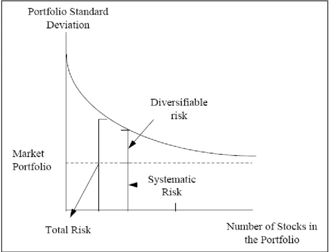
Figure 2.1 The standard deviation of portfolio return as a function of the number of securities in the portfolio. (Fama, E.F., Foundation of Finance, 1976, 253-254.)
The figure represents how a portfolio risk reduces with the increasing number of stocks in a portfolio. In fact, adding a new stock eliminates the firm specific risk of other stocks and thus reduces the diversifiable risk Fama (1976) has illustrated this above result empirically, as it is shown shortly graph above. He randomly selected 50 New York Stock Exchange (NYSE)
approximately 11%. Then this security combined with another randomly selected security to form an equally weighted portfolio of two securities. The result was decrease of standard deviation to around 7 %. Next, step by step more randomly selected securities were added to the portfolio until 50 securities included. All the diversifications was obtained after the first 10-15 securities selected, also the portfolio standard deviation quickly approached a limit that is almost equal to the average covariance of all securities.
On the other hand, adding new stocks do not help in reducing the portfolio risk after a certain number of stocks. The remaining risk, which cannot be eliminated, is the non-diversifiable risk, which mainly depends on the macro factors that affect all the firms whose stocks are included in the portfolio.
Risk is formulized by William Sharpe as;
rp p
rm
ep 2 2 2 2 Equation (2.7)
rp 2 Total Risk
m p 2 r 2 = Systematic risk in other words non-diversifiable risk or market risk
ep2
= Unsystematic risk, diversifiable risk or specific risk
p
= The beta coefficient, the relative volatility of a stock, fund, or other security in comparison with the market as a whole.
2.2 Measuring Risk for a Single Asset and Portfolio Risk Composed of Two Assets
of distribution, how far they are away from the mean. To measure variance, we must have some distribution/ possibility of asset returns or expected returns.
The variance of a random variable or distribution is the expected, or mean, value of the square of the deviation of that variable from its expected value or mean. It is calculated as follows:
1 2 2
N xi Equation (2.8)where, x is random variable i is the expected value or the mean and N is the size or observation. And standard deviation is shown as below:
1 2
N xi Equation (2.9)For a single asset that its probability distribution is given or known, risk or standard deviation is calculated as follow:
2 1 ) ( i i n i i
P R R Equation (2.10) i = standard deviation of asset ( i )
i P = probability i R = return ) (Ri
E = Expected return of asset ( i ) under given probabilities and it is formulized as;
R P R
On the other hand calculation of a portfolio risk is different from calculation of a single asset risk. To make an easier explanation, assume a portfolio composed of two assets; asset 1 ( i ) and asset 2 ( j ) and a proportion denoted by W is invested in the asset ( i ) and the rest 1-i Wi
denoted by Wj is invested in the asset ( j ). The rate of return on this portfolio, Rp, is calculated as follow: j j i i p W R W R R * * Equation (2.12)
In general terms, for a portfolio composed of “k” assets; expected returns for that portfolio could be expressed as;
Rp Wk E
RkE * Equation (2.13)
where k = 1, 2, … k
And variance of two assets portfolio is;
i i
j i j j i i p W W 2WW Cov R,R 2 2 2 2 2 Equation (2.14)As it is shown formula above a new term “Cov”- covariance which is a measure of how much two variables change together. In other words the extent to which two variables vary together (co-vary) could be measured by their covariance.
where expected returns=E(Ri)
Pk *Ri and P is different probabilities of expected k situations. And also j i j i j i Cov, * *, Equation (2.16)where is the correlation between assets or variables ( i ) and ( j ).i,j
The value of the covariance, correlation coefficient, is interpreted as follows:
If the result of the covariance calculation is zero then the two variables are not related to one another. When the result is positive then the two variables have moved in the same direction. The larger the result the more strongly related the two variables are. If the result is negative then the two variables have a negative relationship with one another, that is are moving in opposite directions.
Thus,
If cov(i, j) is < 0, then i and j move in opposite direction If cov(i, j) is > 0, then i and j move in same direction
Figure 2.2 Scattered correlation graphs between two variables (http://www.gseis.ucla.edu/courses/ ed230bc1/notes1/var1.html)
The more tightly the points are clustered together the higher the correlation between the two variables and the higher the ability to predict one variable from another -the symbol r generally is used to stand for the correlation-. Also it is known as, the Pearson correlation coefficient or just the correlation coefficient.
Correlation coefficients can take on any value between -1 and +1, with + and - 1 representing perfect correlations between the variables. And a correlation of zero represents no relationship
A rule of thumb for interpreting correlation coefficients: Correlation Interpretation 0 to 0.1 trivial 0.1 to 0. 3 small 0.3 to 0.5 moderate 0.5 to 0.7 large 0.7 to 0.9 very large
Correlations are interpreted by squaring the value of the correlation coefficient. The squared value represents the proportion of variance of one variance that is shared with the other variable, in other words, the proportion of the variance of one variable that can be predicted from the other variable.
2.3 Measuring Risk for a Portfolio Composed of “n” Number of Assets
The beta coefficient is a relevant risk measure if the market model has had wide acceptance. Theoretical justification for this risk measure can be derived from the portfolio approach which makes the basic assumption that investors evaluate the risk of a portfolio as a whole rather than the risk of each asset individually. Also, the portfolio approach concludes that the risk of a portfolio should be measured by the covariability of its return of the market portfolio. Thus the market risk of an individual security, as it contributes to the portfolio covariability, is the appropriate measure of risk for that security since nonmarket related risk can be eliminated by the aggregation of securities in a portfolio (Klemkosky and Martin, 1975).
Risks in investment means that future returns are unpredictable. The spread of possible outcomes is usually measured by standard deviation. Most individual stocks have higher standard deviations, but much of their variability represents unique risks that can be eliminated
exposed to variations in the general level of the market. A security’s contribution to the risk of a well-diversified portfolio depends on how the security is reliable to be affected by a general market decline. This sensitivity to market movements is known as beta. Beta measures the amount that investors expect the stock price to change for each additional 1 percent change in the market.
Previously we have mentioned measure of risk of a portfolio composed of two assets, and here we will make our explanations for three assets in order to show variance and covariance of a portfolio then we will shortly explain the “beta” which represents the risk, formula of portfolio.
Suppose a three assets portfoliow ,1 w ,2 w to be the percentages invested; 3 E
R1 , E
R2 ,
R3E to be the expected returns; 2 1 , 2
2 , 2
3
to be the variances; , 12 , 23 to be the 13 covariance and finally R , 1 R , 2 R to be the random returns of a three assets portfolio 3
respectively. The formulation of the portfolio mean return, as also mentioned previously, will be;
R E
w1R1 w2R2 w3R3
E p Equation (2.17)
or reversing the formula as
R w1E
R1 w2E
R2 w3E
R3E p Equation (2.18)
The expected portfolio return is simply a weighted average of the expected return on individual assets, which can be written shortly;
The definition of portfolio variance for three assets is the expectation of the sum of the mean differences squared;
2
3 3 2 2 1 1 3 3 2 2 1 1R w R w R w E R w E R w E R w E R Var p E
w1
R1 E
R1
w2
R2 E
R2
w3
R3 E
R3
2
3 3 2 2 3 2 3 3 1 1 3 1 2 2 1 1 2 1 2 3 3 2 3 2 2 2 2 2 2 1 1 2 1 2 2 2 R E R R E R w w R E R R E R w w R E R R E R w w R E R w R E R w R E R Ew
1 3
2 3
2 3
3 1 2 1 2 1 3 2 3 2 2 2 1 2 1 , 2 , 2 , 2 R R COV w w R R COV w w R R COV w w R Var w R Var w R Var w Equation (2.20)Shortly the portfolio variance is a weighted sum of variance and covariance terms and could be rewritten as;
3 1 3 1 i j ij j i p ww R Var Equation (2.21)where w and i wj are the percentages invested in each asset, and is the covariance of asset i ij with asset j.
When we replace the three assets with N, Equations (2.20) and (2.21) could be used as a general representation of the mean and variance of a portfolio with N assets. These equations could be also rewritten in matrix form, which for two assets looks like this:
R
E
R E R
w RWEquation (2.23)
The expected portfolio return is the
1xN
row vector of expected returns,
E
R1 ,E R2
Rpostmultiplied by the
N x1
column vector of weights held in each asset,
w1w2
W . The variance is the
N xN
variance-covariance matrix, , premultiplied by the vector of weights,W. As it seen that the matrix definition of the variance is identical to Equation (2.21) when the variance-covariance matrix is firstly postmultiplied by the column vector of weights in order to get
2 2 2 1 2 1 2 1 2 1 1 1 2 1 w w w w w w R Var p Equation (2.24)then postmultiplied the second vector times the first,
R w1211 w1w212 w2w121 w2222Var p Equation (2.25)
Finally terms are collected and seen that this is equal to
i j ij N j N i p ww R Var
1 1 where N 2 Equation (2.26)agents have preferences over consumption bundles and will always choose the most preferred bundle subject to applicable constraints. Preferences are relationships between alternative consumption "bundles". These can be represented graphically using "indifference curves", as illustrated below in Figure (2.3) Focusing now on the preferences of a single consumer, the indifference curve is a line which connects all combinations of two goods x and y between which the consumer is indifferent. As this curve is drawn, we have represented an agent with "well-behaved preferences": at any allocation, more is better (monotonicity), and averages are preferred to extremes (convexity). Exactly one such indifference curve goes through each positive combination of x and y. Higher indifference curves lie to the "north-east".
Figure 2.3 Indifference curve
If we wish to characterize an agent's preferences, the "marginal rate of substitution" (MRS) is a useful point of reference. At a given combination of x and y, the marginal rate of substitution is the slope of the associated indifference curve. As drawn, the MRS increases in magnitude as we move to the northwest and the MRS decreases as we move to the south east. The intuitive understanding is that the MRS measures the willingness of the consumer to trade off one good for the other. As the consumer has greater amounts of x, she will be willing to trade more units of x for each additional unit of y.
An important feature of the optimal portfolio that investors choose in order to maximize their utility is that the marginal rate of substitution between their preference for risk and return represented by the indifference curves must equal the marginal rate of transformation offered by the minimum variance opportunity set.
Selecting the most desirable portfolio involves the use of indifference curves. These curves represent an investor's preferences for risk and return. It can be drawn on a two-dimensional graph, where the horizontal axis usually indicates risk as measured by variance or standard deviation and the vertical axis indicates reward as measured by expected return. Using variance as relevant risk measure comes from Markowitz's (1952), and is always used in practice, although other possibilities have been considered. This definition gives us the following properties, assuming we have a rational investor:
All portfolios that lie on the same indifference curve are equally desirable to the investor (even though they have different expected returns and variance.)
An investor will find any portfolio that is lying on an indifference curve that is further northwest to be more desirable than any portfolio lying on indifference curve that is not as far northwest.
Generally it is assumed that investors are risk averse, which means that the investor will choose the portfolio with the smaller variance given the same return. Risk-averse investors will not want to take fair gambles (where the expected payoff is zero). These two assumptions of nonsatiation and risk aversion cause indifference curves to be positively sloped and convex. Risk aversion which, intuitively, implies that when facing choices with comparable returns, agents tend chose the less-risky alternative (Friedman and J. Savage, 1948).
Risk aversion (the symbol A is used) is measured as the additional marginal reward an investor requires to accept additional risk. Formulized as;
d R dE
A ( ) Equation (2.27)
Figure 2.4 Indifference curve of absolutely risk insensitive investor
Indifference curves of an investor who is absolutely insensitive against risk are parallel to the horizontal axis and slope of the line is equal to zero. For these kinds of investors, return level should be fixed on a certain point regardless of level of risk. Indifference curve of an investor who is absolutely insensitive against risk as shown above whatever the level of risk is expected return is fixed at the point ofE(rB).
Figure 2.5 Indifference curve of absolutely risk sensitive investor
Indifference curve of this type of investors is parallel to the vertical axis. For these kinds of investors, risk level should be fixed on a certain point regardless of level of return. They do not like to take risk and they want to make their investments in safer instruments. Indifference curve of an investor who is absolutely sensitive against risk as shown above whatever the level of return is acceptable risk level for that investor is . A
In real life, it is unlikely to come across such investors who are absolutely sensitive or insensitive against risk. In real life these types of investors are available who emphasize a little more on risk compared to return or regard return more important than risk.
Figure 2.6 Indifference curve of risk averse investor
The above risk indifference curve specifies the type of investors who do not like to take risk. Slope of this curve is high. As it is shown on the graph, a small increase in the risk would be acceptable only a greater growth in return. These types of investors do not behave recklessly and they escape from risk. Therefore these types of investors make their investments in securities which are less risky and bring more stable return.
This figure shows the type of investors who like to take risks. A small increase in return is satisfactory for these types of investors compared with a greater increase in risk. They do not avoid making investment in riskier securities. As shown above, risk lover investor accepts to take a higher risk in order to achieve 2 E(r1) return which is a little higher thanE(r2).
As a result, attitudes and preferences of capital owners determine making investment in which securities according to risk and return levels.
2.5 Return and Its Calculation
Investors take risk in order to get a satisfactory gain for themselves. In other words; risk is endured for return. However return may always not be gain but also loss for investors. Therefore, return could be defined as the gain or loss of a security in a particular period. It consists of the income and the capital gains relative on an investment.
Attention on returns rather than prices is focused because for an average investor, financial markets may be considered close to perfectly competitive, so that size of the investment does not affect price changes. Returns also have more attractive statistical properties than prices Lucas (1978).
Calculation of return may vary. Arithmetic mean and geometric mean could be used or logarithmic functions could be taken into account while return calculation. In our analysis log returns will be taken into consideration.
Arithmetic average is formulized as;
n
i R Rate of return n Number of period Geometric mean = n
1 1
1 2
1
1 n R R R Equation (2.29)where R is again defined as the rate of return.i
Return simply formulized as;
Percentage of return= (Value at ending period – Value at beginning period)/ Value at beginning period; which is the price of percentage change for a period of time. The return,R , i
-for an asset priced P at the date t - on the asset between dates t t1and t is defined as;
1 1 t t t P P R Equation (2.30)
The simple gross return on the asset is just one plus the net return, 1Rt. And from this equation it is apparent that the asset’s gross return over the most recent k periods from date
k
t to date t , or 1Rt(k)will simply be equal to the product of the k single period returns from t k1 to t which is formulized as;
) 1 ( ) 1 ( ) 1 ( ) ( 1Rt k Rt Rt1 Rtk1 k t t k t k t t t t t t t P P P P P P P P P P 1 3 2 2 1 1 Equation (2.31)
and its net return over the most recent k periods, Rt(k), is equal to its k period gross return minus one. These multiperiod returns are called compound returns. Although returns are scale
The continuously compounded return or log return, r of an asset is defined to be the natural t
logarithm of its gross return
1Rt
;
1 log 1 log t t t t P P Rr or logPt logPt1 Equation (2.32)
where “P” represents price of a stock.
The advantages of continuously compounded returns become clear when we consider multiperiod returns, since
log
1 t( )
log
1 t
1 t1
1 tk1
t k R k R R R
r
log
1Rt
log
1Rt1
log
1Rtk1
rt rt1 rtk1, Equation (2.33)
and hence the continuously compounding multiperiod return is simply the sum of continuously compounded single-period returns. Compounding, a multiplicative operation, is converted to an additive operation by taking logarithms. However, this simplification is not just in reducing multiplication to addition, but more in the modeling of the statistical behavior of asset returns over time.
On the other hand, continuously compounded returns do have disadvantages such as not linear in portfolio return and unrealistic approach. The simple return on a portfolio of assets is a weighted average of the simple returns on the assets themselves, where the weight on each asset is the share of the portfolio’s value invested in that asset. In empirical applications this problem is usually minor. When returns are measured over short intervals of time, and are
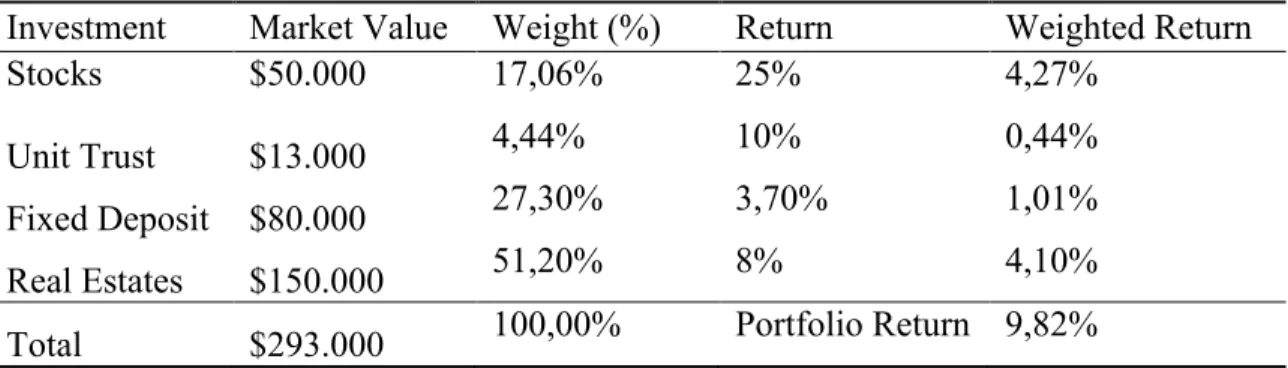
The return of portfolio is the simply weighted mathematical average of a series of returns generated over a period of time. For example, you invest in several asset classes and get different return from each other, so your overall investment portfolio is;
Return of portfolio
W1R1
W2 R2
WnRn
Equation (2.34) where W , 1 W and 2 W stand for the weightings in % of assets, for asset 1 to n, in the portfolio. nWhereas, R , 1 R and 2 R are returns for the respective assets, 1 to n, in the portfolio. More n
than half is invested in real estates.
Table 2.1 Overall portfolio return
Investment Market Value Weight (%) Return Weighted Return
Stocks $50.000 17,06% 25% 4,27%
Unit Trust $13.000 4,44% 10% 0,44%
Fixed Deposit $80.000 27,30% 3,70% 1,01%
Real Estates $150.000 51,20% 8% 4,10%
Total $293.000 100,00% Portfolio Return 9,82%
Weight of stocks = 50k/293k = 17.06%
Weighted return of stocks = 25% x 17.06% = 4.27%
Overall portfolio return = 4.27 + 0.44 + 1.01 + 4.10 = 9.82%
When probability distribution is known expected return for a single asset as formulized previously will be;
k i n k k i P R R E( ) * 1
Equation (2.35)And expected return of the portfolio will be defined weighted average of the assets invested in that portfolio which is shown as;
i n i i p W E R R E
1 ) ( Equation (2.36)PART 3 MODERN PORTFOLIO THEORY 3.1 The Theory and Its Assumptions
Modern portfolio theory (MPT) was pioneered by Harry Markowitz in his paper "Portfolio Selection," published in 1952 and it was considered an important advance in the mathematical modeling of finance which tries to maximize return and minimize risk by choosing different assets.
Modern portfolio theory states that the risk for individual asset returns has two components, systematic and unsystematic risk which details explained in part 2.
Markowitz’s (1952) theory says that it is not enough to look at the expected risk and return of one particular asset. Through investing in more than one asset, an investor can achieve the benefits of diversification.
According to the theory, expected return of the investors and risk values are the two basic variables which determine their portfolio choice. Markowitz explains that main purpose of portfolio creation is to minimize risk while maximizing return. In this theory, number of assets included in the portfolio has as great importance as correlation between these asset returns with each other. For example marginal benefits of putting two assets in a portfolio which their returns are moving in same direction will not be high as explained in part 2.2 correlation sections.
In modern portfolio theory expected return and risk for any portfolio is formulized as following:
i i n i p E r w r E
1 Equation (3.1)3.1.1 Assumptions of modern portfolio theory
- The theory assumes that investors are risk averse, meaning that given two assets that offer the same expected return, investors will prefer the less risky one. Thus, an investor will take on increased risk only if compensated by higher expected returns. Conversely, an investor who wants higher returns must accept more risk. The exact trade-off will differ by investor based on individual risk aversion characteristics. The implication is that a rational investor will not invest in a portfolio if a second portfolio exists with a more favorable risk-return profile – i.e., if for that level of risk an alternative portfolio exists which has better expected returns.
- Investors take into consideration only risk and return while making their investment decisions. MPT further assumes that the investor's risk / reward preference can be described via a quadratic utility function. The effect of this assumption is that only the expected return and the volatility (i.e., mean return and standard deviation) matter to the investor. The investor is indifferent to other characteristics of the distribution of returns, such as its skew or kurtosis.
- Main aims of the investors are to maximize expected utilities.
- There is no transaction cost.
- Expectations of investors are homogeneous.
- Capital markets are efficient. Market efficiency states that the price already reflects the all available information. It assumes that all news and information which effecting the price of the assets are reflected to the market immediately and accurately. Therefore a market cannot be outperformed because all available information is already built into all asset prices. And also it states that forecasting for future in other words technical analysis through looking at
3.2 Efficient Frontier
Markowitz has brought the concept of “efficient frontier” to the portfolio theory. One of its largest contributions was its demonstration of the power of diversification. It is assumed that data for a collection of assets which the return rates and standard deviations are graphed for these assets, and for all portfolios it could be gotten by allocating among them. Markowitz showed that through this way it could be achieved a region bounded by an upward-sloping curve, which he called the efficient frontier.
Figure 3.1 Efficient frontier (http://www.investopedia.com/terms/e/efficientfrontier.asp)
It's obvious that for any given value of standard deviation, investors would like to choose a portfolio that gives the greatest possible rate of return; so investors always want a portfolio that lies up along the efficient frontier, rather than lower down, in the interior of the region. This is the property of the efficient frontier that it is where the best portfolios are lie on the curve. The other important property of the efficient frontier is that it is curved, not straight. This curve is the key to how diversification lets investors improve reward-to-risk ratio. The
to risk. Each unit of risk added to a portfolio gains a smaller and smaller amount of return. The smaller the covariance between the assets included in portfolio the more out of sync they are -- the smaller the standard deviation of a portfolio that combines them. The ultimate would be to find assets with negative covariance.
In Markowitz model, investors should make “n” number of expected returns, “n” number of standard deviation, “ n (n-1) / 2 “ number of covariance , in total “ n (n+3) / 2 “ number of data predictions which it is difficult practically in order to get efficient frontier.
3.3 Determination of Optimal Portfolio on Efficient Frontier with the Help of Indifference Curves
The efficient frontier consists of the set of all efficient portfolios that yield the highest return for each level of risk. The curve showing the expected return and risk preferences of investors is called indifference curve. Optimal portfolio could be determined with the help of these two curves. As it is known all portfolios located on the efficient frontier line is optimum.
For the investors choosing which of the portfolio on this line depends on their preferences and risk attitudes that determines their indifference curves. For an investor optimal portfolio is the portfolio, lying on the efficient frontier, which provides the highest utility. This appropriate portfolio selection realizes on the point where the indifference curve of the investor is tangent to the efficient frontier.
Figure 3.2 Determination of optimal portfolio on efficient frontier
As shown figure above, optimal portfolio is on the point of “A” where the indifference curve is tangent to the efficient frontier. For instance, at the point of “A” risk level is and 1 expected return is E
R and for an investor who has these risk and return expectation levels portfolio “A” is the optimal portfolio for that investor.Figure 3.3 Optimal portfolio determination under different risk preferences of investors
Investors choose the most appropriate portfolio at the any point on the Markowitz’s efficient frontier depending on their risk aversion degrees. Let us assume “a” and “b” two kind of investors, investor “a” dislike risk compared to investor “b”. For these investors points A and B are the optimal portfolios respectively graphed on the figure above. Investor “b” is more risk lover than investor “a”, therefore risk and expected return of his portfolio are higher than portfolio “A”.
PART 4 CAPITAL MARKET THEORY
The capital market theory builds upon the Markowitz portfolio model. In Harry Markowitz’s efficient frontier hypothesis just risky assets are taken into consideration in order to build efficient portfolio set, however in this model a new efficient set is constructed by adding risk free assets. The prominent characteristic of this model is concept of risk-free asset.
Assets like treasury bills and bonds which have a certain future return are considered to be risk-free because they are backed by the government. These securities are considered to be risk-free because the likelihood of governments defaulting is extremely low. Investing in these kinds of financial instruments eliminates default risk. However, these instruments could carry other types of risk such as inflation risk (Dimson and others, 2002).
The theory figure outs the rates of return for efficient portfolios depending on the risk-free rate of return and the level of risk for a particular portfolio. It is derived by drawing a tangent line from the intercept point on the efficient frontier to the point where the expected return equals the risk-free rate of return. The line is created in a graph of all possible combinations of risky and risk-free assets.
4.1 Assumptions of Capital Market Theory
- All investors are efficient investors who follow Markowitz idea of the efficient frontier and choose to invest in portfolios along the frontier.
- Investors could borrow and lend for any amount of money at the risk-free rate
- All investors have homogeneous expectations and have the same probability for outcomes, in other words all investors have the same probability for outcomes while determining the
- The investment time horizon is equal for all investors, investors have equal time horizons for the chosen investments.
- All investment alternatives have the property of divisibility and assets are infinitely divisible. This indicates that fractional shares could be purchased and the stocks could be infinitely divisible.
- There are no taxes and transaction costs which in turn investors’ results are not affected by taxes and transaction costs.
- There is no change in inflation and interest rates or all modifications are fully predictable. Inflation does not exist and returns are not affected by the inflation rate in a capital market as none exists in capital market theory.
- There is no mispricing within the capital markets and the markets are efficient.
(Copeland and others, 2004)
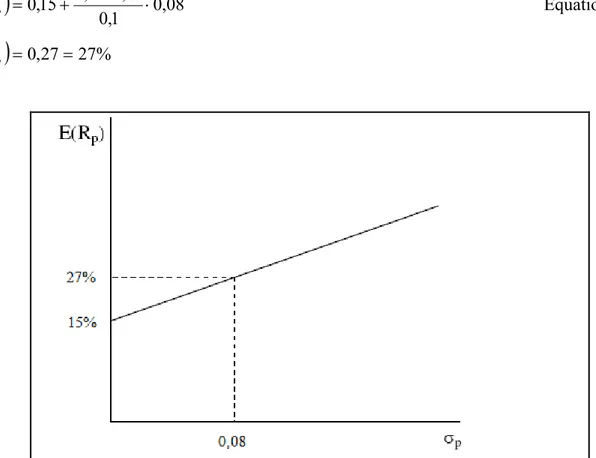
4.2 The Capital Market Line (CML)
According to the capital market assumptions, rational investors would like to make their investment on capital market line. In capital market theory relation between risk and expected return for efficient portfolios is explained by capital market line. This line is shown and formulized together with an example below:
Figure 4.1 Capital market line
p m f m f p r r E R r E Equation (4.1)
rp E Expected return of the portfolio
f
R Return of risk-free asset
rm E Expected return of market
m
Standard deviation-risk- of the market
p
Standard deviation-risk- of the portfolio
For instance; return of risk-free asset
rf is 15%, expected return of the market
E
rm
is 30% with a standard deviation
0,1 and standard deviation of efficient portfolio
is0,08 in this case according to the capital market line formulation expected return of efficient portfolio is calculated as below;
0,08 1 , 0 15 , 0 3 , 0 15 , 0 p r E Equation (4.2)
rp 0,2727% EFigure 4.2 Expected return calculation of a portfolio on capital market line
CML consists of the market portfolio and free combination. Together with adding risk-free asset to model curve shape of the Markowitz’s efficient frontier is replaced by a linear line. CML is a line, extended from risk-free rate to the market portfolio, which shows the relationship between the return and standard deviation of the portfolio and only efficient portfolios are located on the capital market line.
in risky and risk-free assets will be different from each other. This market portfolio represents the most appropriate combination of every accessible asset in the market available to investors, which is consisted proportionally weighted sum of their market values.
On the capital market line only market portfolio “M” which is consisted of risky assets is efficient, whereas in the Markowitz’s model large number of risky portfolios could be optimal portfolios. Market portfolio is superior to all other portfolios. In market portfolio, all assets such as Treasury bill, government bonds, stocks, options and etc. are included. And it could be claimed that market portfolio contains only systematic risk since it is a very well diversified portfolio (Konuralp, 2001)
Shortly, an investment in market portfolio M (the tangency point) and the riskless asset is an optimal strategy for all investors. Investors will only differ in the relative proportions invested in the two components. The following figure illustrates that both investor “A” and investor “B” will prefer this strategy to an investment in risky assets alone. Investor “A”, who is more averse towards risk, invests a higher proportion of his wealth in the riskless asset than does investor “B”. From the figure, investor “A” invests about half his wealth in the riskless asset and half in the portfolio of risky assets “M”. Investor “B” invests all his wealth in the portfolio of risky assets “M”, then borrows at the riskless rate,rf, and invests this in the portfolio of risky assets as well.