Selçuk J. Appl. Math. Selçuk Journal of Vol. 11. No.2. pp. 109-122, 2010 Applied Mathematics
Numerical Study of Heat and Mass Transfer in Magneto Hydrody-namic Flow past a Vertical Plate with Constant Injection and Heat Flux
V. Ambethkar
Department of Mathematics, University of Delhi, Delhi 110 007, India e-mail: vamb ethkar@ m aths.du.ac.in, vamb ethkar@ gm ail.com
Received Date: April 7, 2010 Accepted Date: August 15, 2010
Abstract. We have studied heat and mass transfer in an unsteady MHD flow of an incompressible, electrically conducting, and viscous fluid. It is considered that the influence of the uniform magnetic field normal to the flow. Numerical results for temperature, velocity, concentration, have been obtained and shown graphically for suitable parameters like Grashoff number, mass Grashoff number, Prandtl number and Schmidt number. Rate of heat transfer and mass transfer are studied. The results obtained are discussed with the help of graphs and tables to observe effect of various parameters concerned in the problem under investigation. The main conclusions of this study have been given.
Key words: Injection; Heat Flux; Heat and Mass transfer; Numerical solution. 2000 Mathematics Subject Classification. 80A20.
1. Introduction
Investigation of magneto-hydrodynamic (MHD) flow for an electrically conduct-ing fluid past a heated surface has attracted the interest of many researchers in view of its important applications in many engineering problems such as plasma studies, petroleum industries, MHD power generators, cooling of nu-clear reactors, the boundary layer control in aerodynamics, and crystal growth. This study has been largely concerned with the flow and heat and mass trans-fer characteristics in various physical situations. Vajravelu and Hadjinicolaou (1997) studied convective heat transfer in an electrically conducting fluid at a stretching surface with uniform free stream. Anjalidevi and Kandasamy (1999) investigated effects of chemical reaction, heat and mass transfer on laminar flow along a semi infinite horizontal plate. Magnetic field effects on the free convec-tion and mass transfer flow through porous medium with constant succonvec-tion and
constant heat flux was studied by Acharya et al. (2000). Sahoo et al. (2003) have studied MHD unsteady free convection flow past an infinite vertical plate with constant suction and heat sink. Heat and mass transfer in MHD flow of a viscous fluid past a vertical plate under oscillatory suction velocity was in-vestigated by Singh et al. (2003). Chamkha (2004) inin-vestigated unsteady MHD convective heat and mass transfer past a semi-infinite vertical permeable moving plate with heat absorption. Hazem (2006) studied on the effectiveness of uni-form suction and injection on unsteady rotating disk flow in porous medium with heat transfer. Chaudhary and Jha (2008) have studied heat and mass transfer in elastico-viscous fluid past an impulsively started infinite vertical plate with Hall effect. Mahdy et al. (2009) have investigated heat and mass transfer in MHD free convection along a vertical wavy plate with variable surface heat and mass flux. Samad and Mohebujjaman (2009) have studied MHD heat and mass transfer free convection flow along a vertical stretching sheet in presence of magnetic field with heat generation.
Because of enormous practical applications of injection to problems of boundary layer control, thermal protection of high energy flows and recently to those of seeding processes to enhance possible MHD effects and due to intricacy analysis to investigate combined effects of heat and mass transfer with injection of an MHD flow, we have been fascinated to and motivated towards this direction. Our main purpose is to investigate numerically the problem of combined heat and mass transfer of an unsteady MHD flow past an infinite plate with injec-tion. The results of this study are discussed for various numerical values of the parameters which suits for the case of injection.
2. Mathematical Formulation
Here an unsteady two dimensional free convective flow of an electrically con-ducting viscous and incompressible fluid past an infinite, porous and vertical plate with constant injection and heat flux is considered. A magnetic field 0
is applied perpendicular to the plate. A system of rectangular coordinate axes o 111is taken such that 1= 0 on the plate and 1is along its leading edge.
All the fluid properties are considered. The influence of the density variation with temperature is considered only in the body force term. Its influence in other terms of the momentum and the energy equations is assumed to be negli-gible. The variation of expansion coefficient with temperature is considered to be negligible. This is the well-known Boussinesq approximation. Thus, under these assumptions, the physical variables are functions of 1 and 1 only and
the problem is governed by the following system of equations continuity equation : 1 1 = 0 (1) momentum equations : 1 1 + 1 1 1 = (1− ∞)+ 2 1 2 1 − 2 01 (2)
energy equation : 1 1 + 1 1 1 = 2 1 2 1 (3)
mass transfer equations : 1 1 + 1 1 1 = 0 2 1 2 1 (4)
The initial and boundary conditions of the problem are 1≤ 0 1(1 1) = 0 1(1 1) = ∞ 1(1 1) = ∞; (5) 1 0 1(0 1) = 0 1(0 1) = + (− ∞)11 1(0 1) = ∞+ (− ∞)1 at 1= 0; (6) 1 0 1(∞ 1) → 0 1(∞ 1) → ∞ 1(∞ 1) → ∞ as 1→ ∞ (7)
Since the plate is assumed to be porous type and through it suction with uniform velocity occurs, equation (1) integrates to
1= −0
which is the constant suction velocity. Here, is the velocity of the fluid, 1 is
the temperature of the fluid, is the dimensionless temperature, is the
tem-perature of the fluid near the plate, ∞is the temperature of the fluid far away from the plate, 1 is the concentration of the species, is the concentration
near the plate, ∞ is the concentration far away from the plate, is dimen-sionless concentration, is the acceleration due to gravity, is the coefficient of volume expansion for heat transfer, 0 is the coefficient of volume expansion for concentration, is the kinematic viscosity, is the scalar electrical conductiv-ity, is the frequency of oscillation, is a constant, 0 is the applied uniform
magnetic field, is the density of the fluid, is the thermal conductivity, is the injection parameter, 0 is the molecular diffusivity, and is the time. From equation (1) we observe that 1 is independent of space co-ordinates and
and parameters. (8) = 1 2 0 4 = 01 4 = 1 0 =1− ∞ − ∞ = 1− ∞ − ∞ = = 0 = 2 0 2 0 = (− ∞) 3 0 = 1 0 = 0(− ∞) 3 0 =1 2 0
Now taking into account equations (5), (6), (7) and (8), equations (2), (3) and (4) reduce to the following non-dimensional form
(9) − = 2 2 + − + − = 2 2 (10) − = 2 2 (11) with ≤ 0 ( ) = 0 ( ) = 0 ( ) = 0; (12) 0 (0 ) = 0 (0 ) = 1 + (13) (0 ) = at = 0; 0 (∞ ) = 0 (∞ ) = 0 (∞ ) = 0 as → ∞ (14)
The Grash of number 0 represents external cooling of the plate and 0
denotes external heating of the plate. the modified Grshof number, the
3. Method of solution
In order to solve these unsteady, linear coupled equations (9) to (11) under the conditions (12) to (14), an implicit method of Crank-Nicolson type has been employed. To obtain the finite difference equations, the region of the flow is divided into a grid of mesh points ( ). The values of the dependent variables
and at the nodal points along the plane = 0 are given by (0 ), (0 ) and (0 ) hence are known from the boundary conditions. Let ∆ and ∆ represents the uniform step lengths in and directions. We need a scheme to find single values at next time level in terms of known values at an earlier time level. A forward difference approximation for the first order partial derivatives of and with respect to and and a central difference approximation for the second order partial derivative of and with respect to are used. On introducing finite difference approximations for
, , 2 2, , , 2 2, , , 2 2 as µ ¶ = +1− (∆) ; µ ¶ =+1+1−−1+1++1−−1 4(∆) ; µ ¶ = +1− (∆) ; µ ¶ =+1+1−−1+1++1−−1 4(∆) ; µ ¶ = +1− (∆) ; µ ¶ =+1+1−−1+1++1−−1 4(∆) ; µ 2 2 ¶ = +1− 2+ −1+ +1+1− 2+1+ −1+1 2(∆)2 ; µ 2 2 ¶ =+1− 2+ −1+ +1+1− 2+1+ −1+1 2(∆)2 ; µ2 2 ¶ = +1− 2+ −1+ +1+1− 2+1+ −1+1 2(∆)2 (15)
The finite difference approximation of equations (9) to (11) are obtained on substituting equation (15) into equations (9)-(11)
2+1− µ 1 2+ ∆ ∆ ¶ +1+1+ µ ∆ ∆− 1 2 ¶ −1+1 =¡1 2+ ∆ ∆ ¢ +1+ ³ −∆ ∆+ 1 2 ´ −1+∆+∆−∆ (16) µ 1 + ¶ +1+ µ ∆ ∆− 2 ¶ −1+1− µ ∆ ∆+ 2 ¶ +1+1 = µ ∆ ∆+ 2 ¶ +1+ µ 2 − ∆ ∆ ¶ −1+ µ 1 − ¶ (17)
µ 1 + ¶ +1+ µ ∆ ∆− 1 2 ¶ −1+1− µ ∆ ∆+ 1 ¶ +1+1 = µ 2 + ∆ ∆ ¶ +1+ µ 2 − ∆ ∆ ¶ −1+ µ 1 − ¶ (18) 4. Numerical Computations
To get the numerical solutions of the temperature , velocity and concen-tration , we have taken the aid of the computer by developing a code in Mathematica5.0. The logic of the program is divided three steps as follows: Step 1. main, initially it creates three tables to hold the numerical solutions of temperature, velocity and concentration whose coefficients are allotted in the step 2. After this, it calculates the numerical values at the next time level. In order to do this, it uses another sub- module namely Tri-diagonal, which solves the tri-diagonal matrix by using successive over relaxation method with complete pivoting. Further it moves to the step3, for listing the numerical solutions.
Step 2. Coeff Mat, we know that all the terms and their coefficients on right hand side of equations (16), (17) and (18) are known values from initial and boundary conditions. At every time step, for different values of ‘’, the finite difference approximation of equation (18) gives a linear system of equations. Then, for = 0 and = 1 2 − 1, equation (18) gives a linear system of ( − 1) equations for the ( − 1) unknown values of ‘’ in the first time row in terms of known initial and boundary values. This module maintains coefficients of this linear system of equations. Similarly the above process repeats for the remaining equations (17) and (18) to obtain the numerical values of and . Step 3. Tabulation, It lists the numerical solution at every time step level. By making use of and into equation (16), the numerical solutions for ‘’ are obtained.
Code for numerical solutions of temperature profiles for = 0733 for the case
of injection CNgrid[_ _] := Module[{ }, = Table[1 {} {}]; For[ = 1 ≤ + + [[ 1]] = [];]; For[ = 1 ≤ + + [[1 ]] = 1[]; [[ ]] = 2[]; ]; ]; TriDiagonal[0_ 0_ 0_ 0_] := Module[{ = 0 = 0 = 0 = 0 = Length[0] }, For[ = 2 ≤ + +, [[]]= [[]]− ([[−1]][[−1]]) ∗ [[−1]];
[[]]= [[]]− ([[−1]][[−1]]) ∗ [[−1]]; ]; = Table[0 {}]; [[]]= [[]][[]]; For [ = − 1; 1 ≤ ; − − [[]]= ([[]]− [[]]∗ [[+1]])[[]]; ]; Return []; ]; Tabulation : Module[{}, Print["Complete Table"];
Print[" Numerical Solution"];
Print["==============================="]; result=Table["––––—", {( ∗ ) + − 20} {5}]; Input data: = 10; = 01; = 1; = 21; = 41; = −4; [_] = 0; 1[_] = 10; 2[_] = 00; = ( − 1); = ( − 1); [_] = [( − 1)]; 1[_] = 1[( − 1)]; 2[_] = 2[( − 1)]; CNgrid[ ]; = (2∗ )2; = = Table[−1 {−1}]; [[−1]]= [[1]]= 0; = Table[2+(2) {}]; [[1]]= [[]]= 1; = Table[0 {}]; For[ = 2 ≤ , + +, [[1]]= 1[]; [[]]= 2[]; For [ = 2 ≤ − 1 + +, [[]]= (05 − (( ∗ )(4 ∗ ))) ∗ [[−1−1]]+ [[−1]] +(05 + (( ∗ )(4 ∗ )))) ∗ [[+1−1]] +(( ∗ )(4 ∗ )) ∗ ([[+1]]− [−1]]); ]; [[]]=TriDiagonal [ ]; Print[NumberForm[TableForm[ [Transpose[Chop[]]],TableSpacing − {0,2}]]]; Print[TableForm[result,TableSpacing − {0 2}]];
Output:
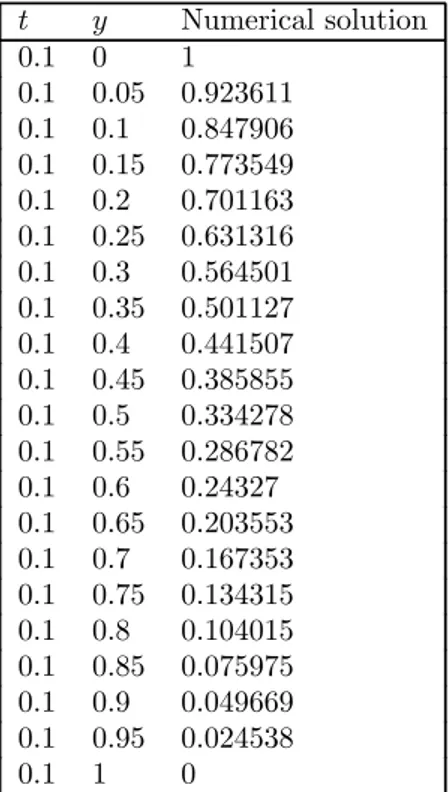
Table 1. Numerical solutions of Temperature profiles for = 0733 for the case of injection
Numerical solution 0.1 0 1 0.1 0.05 0.923611 0.1 0.1 0.847906 0.1 0.15 0.773549 0.1 0.2 0.701163 0.1 0.25 0.631316 0.1 0.3 0.564501 0.1 0.35 0.501127 0.1 0.4 0.441507 0.1 0.45 0.385855 0.1 0.5 0.334278 0.1 0.55 0.286782 0.1 0.6 0.24327 0.1 0.65 0.203553 0.1 0.7 0.167353 0.1 0.75 0.134315 0.1 0.8 0.104015 0.1 0.85 0.075975 0.1 0.9 0.049669 0.1 0.95 0.024538 0.1 1 0
Code for numerical solutions of velocity profiles for = 0733
CNgrid[_ _]:= Module[{ }, = Table[1 {} {}]; = Table[1 {} {}]; For[ = 1 ≤ + + [[1]]= []; [[1]]= []; ]; For[ = 1 ≤ + + [[1]]= 1[]; [[1]]= 1[]; [[]]= 2[]; [[]]= 2[]; ]; TriDiagonal[0_ 0_ 0_ 0_] := Module[{ = 0 = 0 = 0 = 0 = [0] }, For[ = 2 ≤ + + [[]]= [[]]− ([[−1]][[−1]]) ∗ [[−1]]; [[]]= [[]]− ([[−1]][[−1]]) ∗ [[−1]]; = Table[0 {}]; [[]]= [[]][[]]; For[ = − 1 1 ≤ − − [[]]= ([[]]− ([[]]∗ [[+1]]))[[]]; ]; Return[]; ]; Module[{}, Print["Complete Table"];
Print[" Numerical Solution"]; Print["=========================="]; result=Table["–––", {( ∗ ) + − 20} {5}]; Input data: = 10; = 01; = 1; = 1; = 21; = 41; = 2; = 3; = −05; [_] = 0; 1[_] = 10; 2[_] = 00; = ( − 1); = ( − 1); [_] = [( − 1)]; 1[_] = 1[( − 1)]; 2[_] = 2[( − 1)]; CNgrid[ ]; = (2∗ )2; = (2∗ )2; = 05; = = Table[−1 {−1}]; [[−1]]= [[1]]= 0; = Table[2+(2) {}]; = Table[2 + (2) {}]; [[1]]= [[]]= 1; [[1]]= [[]]= 1; = Table[0 {}]; For[ = 2 ≤ + + [[1]]= 1[]; [[]]= 2[]; For [ = 2 ≤ −1 ++ [[]]= [[−1−1]+((2)−2)∗[[−1]+[[+1−1]; ]; [[]]= TriDiagonal[ ]; ]; = Table[0 {}] For[ = 2 ≤ + + [[1]]= 1[]; [[]]= 2[]; For[ = 2 ≤ − 1 + +, [[]]= [[−1−1]]+ ((2) − 2) ∗ [[−1]] +[[+1−1]]+ (4) ∗ ∗ (([[+1−1]]− [[−1]])) +(4) ∗ ∗ (([[+1−1]]− [[−1−1]])) +(∗ ∗ ∗ ([[−1]]+ [[]])) − (2 ∗ ∗ ∗ ∗ [[+1−1]); ]; [[]]= TriDiagonal [ ]; ]; Tabulation: Print[NumberForm[TableForm[ [Transpose[Chop[]]],TableSpacing − {0,2}]]]; Print[NumberForm[TableForm[ [Transpose[Chop[]]],TableSpacing − {0,2}]]]; Comparison[ ]; Print[TableForm[result, TableSpacing − {0,2}]];
Output: numerical solution for velocity profiles for = 0733
Table 2. Numerical solutions of velocity profiles for = 0733
Numerical solution 0.0975 0 1 0.0975 0.05 0.882349 0.0975 0.1 0.853675 0.0975 0.15 0.833967 0.0975 0.2 0.721045 0.0975 0.25 0.671107 0.0975 0.3 0.69668 0.0975 0.35 0.527745 0.0975 0.4 0.364691 0.0975 0.45 0.307724 0.0975 0.5 0.256872 0.0975 0.55 0.211999 0.0975 0.6 0.172823 0.0975 0.65 0.118938 0.0975 0.7 0.159839 0.0975 0.75 0.184943 0.0975 0.8 0.063609 0.0975 0.85 0.04516 0.0975 0.9 0.00889 0.0975 0.95 0.004079 0.0975 1 0
Table 3. Numerical solutions of rate of heat transfer Numerical values of 0.0025 11.69578 0.005 10.4067 0.0075 9.66101 0.01 8.29947 0.0125 7.21477 0.015 7.11348 0.0175 6.60449 0.02 5.991646 0.0225 5.468969 0.025 5.017448 0.0275 4.622961 0.03 4.274846 0.0325 3.964935 0.035 4.686876 0.0375 3.435664 0.04 3.207309 0.0425 2.998585 0.045 2.806863 0.0475 1.629974 0.05 1.466115
Table 4. Numerical solutions of concentration profiles for hydrogen = 022 Numerical solution 0.0025 0 1 0.0025 0.05 1.042285 0.0025 0.1 0.543179 0.0025 0.15 0.283074 0.0025 0.2 0.147522 0.0025 0.25 0.07688 0.0025 0.3 0.040065 0.0025 0.35 0.02088 0.0025 0.4 0.010881 0.0025 0.45 0.005671 0.0025 0.5 0.002955 0.0025 0.55 0.00154 0.0025 0.6 0.000803 0.0025 0.65 0.000418 0.0025 0.7 0.000218 0.0025 0.75 0.000113 0.0025 0.8 5.89E-05 0.0025 0.85 3.02E-05 0.0025 0.9 1.49E-05 0.0025 0.95 6.10E-06 0.0025 1 0
Table 5. Rate of Mass transfer S.No
1 0.22 0.69869 2 0.60 0.85989 3 0.78 0.36896
5. Results and Discussion
For the purpose of discussing the results some numerical solutions are obtained for non-dimensional temperature , velocity and concentration . By using temperature the rate of heat transfer and by using concentration rate of mass transfer is obtained.
The temperature profiles for air (= 0733) for the case of injection are shown
in Table 1. The numerical solutions for the case of injection for temperature have been shown in Table 1. It can be seen from the table that the transient
temperature decreases for the increase of . Similarly temperature field due to variation in for water, mercury etc has been found and observed that
mercury has a stationary temperature. To save the space we are not giving full details as it is obvious to do. The concentration profiles for hydrogen = 022
for the case of injection are shown in Figure 7. The numerical solutions for the case of injection for concentration have been shown in Table 4. It can be seen from the table as well as figure that the transient concentration profiles decreases for the increase of . The concentration profiles due to variation of for gases like oxygen, and water vapor has been found but not giving here
due to almost similar calculations. It can be found that hydrogen can be used for maintaining effective concentration field. The transient velocity profiles for air (= 0733) for the case of injection are shown in Table 2. The numerical
solutions for the case of injection for velocity have been shown in Table 2. It can be seen from the table that the transient velocity profiles decreases for the increase of . While finding velocity profiles numerical values for ,
have been chosen suitably.
From the technological point of view, it is important to know the rate of heat transfer between the plate and the fluid. This can be found by using the non-dimensional quantity, the Nusselt number . The Nusselt number is defined
as negative gradient of the temperature. The numerical values of the Nusselt number against time t are shown in Figure 5 and Table 3. Figure 5 shows the heat transfer for different times. As increases, the rate of heat transfer at the plate decreases gradually. Finally for mass transfer we need the negative gradient of concentration. This is denoted and defined as Schmidt number .
The numerical values of rate of mass transfer in terms of Sherwood number are obtained and have been shown in Table 5. From this table it can be
observed that rate of mass transfer first increases gradually and then decreases as per gradual increase and then decrease of the Schmidt number.
6. Conclusions
The main conclusions of this study are as follows:
(i) The transient temperature decreases for the case of air.
(ii) The transient concentration profiles decreases for the increase of for the case of hydrogen.
(iii) The transient velocity profiles decreases for the increase of for the case of air.
(iv) The rate of heat transfer at the plate decreases gradually.
(v)The rate of mass transfer first increases gradually and then decreases as per gradual increase and then decrease of the Schmidt number.
References
1. Acharya, M., Dash, G.C. and Singh, L.P.(2000): Magnetic field effects on the free convection and mass transfer flow through porous medium with constant suction and constant heat flux, Indian J. Pure Appl. Math., 31, no. 1, 1—18.
2. Anjalidevi, S.P. and Kandasamy, R.(1999): Effects of chemical reaction heat and mass transfer on laminar flow along a semi infinite horizontal plate, Heat Mass Trans-fer, 35, 465—467.
3. Chamkha, A.J.(2004): Unsteady MHD convective Heat and Mass transfer past a semi-infinite vertical permeable moving plate with heat absorption, Int. J. Engg. Sci, 42, 217—230.
4. Chaudhary, R.C. and Jha, A.K.(2008): Heat and mass transfer in elastico-viscous fluid past an impulsively started infinite vertical plate with Hall effect, Latin American Applied Research, 38, 17—26.
5. Hazem, A.A.(2006): On the effectiveness of uniform suction and injection on un-steady rotating disk flow in porous medium with heat transfer, Computational Mate-rials Sci., 38, 240—244.
6. Mahdy, A. Mohamed, R.A. and Hady, F.M.(2009): Heat and mass transfer in MHD free convection along a vertical wavy plate with variable surface heat and mass flux, Latin American Applied Research, 39, 337—344.
7. Singh, A.K., Singh, A.K. and Singh, N.P.(2003): Heat and mass transfer in MHD flow of a viscous fluid past a vertical plate under oscillatory suction velocity, Indian. J. Pure Appl. Math., 34, no. 3, 429—442.
8. Samad, M.A. and Mohebujjaman, M.(2009): MHD heat and mass transfer free convection flow along a vertical stretching sheet in presence of magnetic field with heat generation, Research Journal of Applied Sciences, Engineering and Technology, 1, no. 3, 98—106.
9. Sahoo, P.K., Datta, N. and Biswal, S.(2003): Magnetohydrodynamic unsteady free convection flow past an infinite vertical plate with constant suction and heat sink, Indian J. Pure Appl. Math., 34, no. 1, 145—155.
10. Vajravelu, K and Hadjinicolaou, A.(1997): Convective heat transfer in an electri-cally conducting fluid at a stretching surface with uniform free stream, Int. J. Engng. Sci., 35, nos. 12-13, 1237—1244.