Data sources and computational approaches for generating models of gene regulatory networks

Data Sources and Computational Approaches for 

Generating Models of Gene Regulatory Networks 

B. D. Aguda

G. Craciun

R. Cetin­Atalay 

1  Department of Genetics and Genomics, Boston University School of Medicine  715 Albany Street, Boston, Massachusetts, USA  02118  2  Mathematical Biosciences Institute, The Ohio State University  231 W. 18 th Avenue, Columbus, Ohio, USA  43210  3  Department of Molecular Biology & Genetics, Bilkent University, Ankara, Turkey  and Virginia Bioinformatics Institute, Virginia Polytechnic Institute and State  University, Blacksburg,Virgina,USA 24061

§ _{This author was supported by the National Science Foundation under} Agreement No. 0112050.  OUTLINE  Introduction  Formal representation of GRNs  An example of a GRN: The Lac Operon  Hierarchies of GRN models: From probabilistic graphs to mechanistic models  A guide to databases and knowledgebases on the internet  Pathway Databases & Platforms  Ontologies for GRN modeling  Current Gene, Interaction, and Pathway Ontologies  Whole­cell modeling platforms  Ontology for modeling multi­scale and incomplete networks  An ontology for cellular processes  The PATIKA pathway ontology  Extracting Models from Pathways Databases  Pathway and Dynamic Analysis Tools for GRNs  Global network properties  Recurring network motifs  Identifying pathway channels in networks: extreme pathway analysis  Network stability analysis

Predicting dynamics & bistability from network structure alone  Concluding Remarks

INTRODUCTION  High­throughput data acquisition technologies in molecular biology, including  rapid DNA sequencers, gene expression microarrays and other microchip­based assays,  are providing an increasingly comprehensive parts list of a biological cell.  Although this  parts list may be far from complete at this time, the so­called “post­genomic era” has now  begun in which the goal is to integrate the parts and analyze how they interact to  determine the system’s behavior.  This integration is being facilitated by the creation of  databases, knowledgebases and other information repositories on the internet.  How these  huge amounts of information will be used to answer biological questions and predict  behavior will keep multidisciplinary teams of scientists busy for many years.  A key  question is how the expression of genes is regulated in response to various intracellular  and external conditions and stimuli.  The current paradigm is that the secret to life could  be found in the genetic code; however, the expression of genes and the unfolding of the  regulatory molecular networks in response to the environment may well be the defining  attribute of the living state.  This chapter focuses on gene regulatory networks (GRNs).  A “gene regulatory  network” refers to a set of molecules and interactions that affect the expression of genes  located in the DNA of a cell.  Gene expression is the combination of transcription of  DNA sequences, processing of the primary RNA transcripts, and translation of the  mature messenger RNA (mRNA) to proteins in ribosomes.  This picture is often referred  to as the “central dogma” and it has been the canonical model for the flow of information  from the genetic code to proteins.  These processes are shown schematically as steps  labeled t, r and s in Fig 1.

G  R o  R  P o  P  M t r s m p a  Figure 1.  A schematic representation of a gene regulatory network involving  modules of molecular classes (shown in boxes); the modules shown are the  transcriptional units in the genome (G), primary transcripts (Ro), mature  transcripts (R), primary proteins (Po), modified proteins (P), and metabolites (M).  The labeled steps shown in black lines are transcription (t), RNA processing (r),  translation (s), protein modification (m), metabolic pathways (p), and genome  replication (a).  The feedback interactions shown in gray lines are discussed in  the text.  Filled circles represent either inhibition or activation.

The step labeled m in Fig 1 represents modification of primary proteins to render  them functional; examples would be post­translational covalent modifications (e.g.  phosphorylation) and binding with other proteins or other molecules.  Represented within  the set of steps m are the many regulatory events (other than transcription and translation)  affecting gene expression and the overall physiology of the cell.  The complexity of GRNs may arise from the many possible feedback loops  shown as gray lines in Fig 1.  In step t, proteins could be directly involved in  transcription, as in the case of transcription factors binding to upstream regulatory  regions of genes.  Many RNA and protein molecules cooperate in the translation step s in  Fig 1; examples are tRNA, rRNA, and ribosomal proteins.  The first goal of this chapter is to survey sources of data and other information  that can be used to generate models of GRNs.  The focus is on biological databases and  knowledgebases that are available on the internet, especially those that attempt to  integrate heterogeneous information including molecular interactions and pathways.  The  second goal of this review is to summarize current models of GRNs and how they can be  extracted from biological databases.  Depending on the nature of the data, different  granularities of GRN models can be generated, ranging from probabilistic graphical  models to detailed kinetic or mechanistic models.  A crucial issue in the design of  pathways databases is how to represent information having various levels of uncertainty.  Because of its central importance in GRN modeling, an extensive discussion of pathway  ontology is given.  Lastly, the third goal is to discuss theoretical and computational  methods for the analysis of detailed models of GRNs.  In particular, a summary is given

of various tools already developed in the field of reaction network analysis.  Particular  emphasis of the discussion is on exploiting information on network structure to deduce  potential behavior of GRNs without knowing quantitative values of rate parameters.  FORMAL REPRESENTATION OF GRNS  The GRN of Fig 1 can be formally translated to a set of general dynamical  equations.  The modules (in boxes) in the GRN represent the following classes of  biomolecules:  G  :  vector of all transcriptional units (TUs) involved in the GRN (in terms, for  example, of gene dosage per TU);  Ro  :  vector of primary RNA transcripts corresponding to the TUs in G;  R  :  vector of messenger RNA (mRNA), transfer RNA (tRNA), ribosomal  RNA (rRNA), and other processed RNAs;  Po  :  vector of newly translated (primary) proteins;  P  :  vector of modified proteins;  M  :  vector of metabolites.  Disregarding the replication of the genomic DNA (step a) and the changes in the  metabolome M for now (i.e. assume G and M to be constant), a mathematical  representation of the dynamics of the GRN in Fig 1 would be the following set of vector­  matrix equations:

dRo/dt  =  tG – rRo – d1Ro 

dR/dt  =  rRo – d 2R  [1] 

dPo/dt  =  sR – mPo – d 3Po  dP/dt  =  mPo – d 4P 

The “RNA transcription” matrix t is a diagonal matrix (i.e. all off­diagonal entries are 0)  with the non­zero entries being, in general, functions of R, P, and M as depicted by the  feedback loops in Fig 1.  The “RNA­processing matrix” r is a diagonal matrix with the  non­zero entries being, in general, functions of R and P.  The diagonal matrix s is called  the “protein translation” matrix.  The diagonal matrix m is called the “protein 

modification” matrix (which includes all post­translational modifications, and protein­  protein interactions).  Fig. 1 shows the dependence of s and m to R, P, and M.  The  diagonal matrices di are “degradation” matrices which account for the degradation of 

RNA and protein molecules as well as their transport or dilution.  Because of the general  dependence of the matrices to the variables R, P and M, the above equations are  nonlinear equations in these variables.  An example of a GRN is given next to illustrate the formal representation just  described.  The example also demonstrates the art of modeling and reduction of the  network into minimal mathematical models.

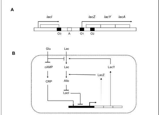
AN EXAMPLE OF A GRN: THE LAC OPERON  The lac operon in the bacterium Escherichia coli is a well­studied GRN.  This  prokaryotic gene network has been the subject of numerous reviews; 1­4  it is discussed  here primarily to illustrate the various aspects of GRN modeling, starting with the  information on genome organization (operon structure) to knowledge on protein­DNA  interactions, protein­protein interactions and the influence of metabolites.  Understanding the lac operon begins by looking at the genome organization of E.  coli.  The complete genome sequence of various strains of this bacterium can be accessed  through the webpage of the National Center for Biotechnology Information  (http://www.ncbi.nlm.nih.gov).  From the homepage menu, clicking Entrez followed by  Genome gives the link to complete bacterial genomes including E. coli.  Genes in the  circular chromosome of E. coli are organized into ‘operons’.  An operon is a cluster of  genes whose expression is controlled by a common set of operator sequences and  regulatory proteins. 5  The genes in the cluster are usually involved in the synthesis of  enzymes needed for the metabolism of a molecule.  Several reviews on the influence of  operon structure on the dynamical behavior of GRNs are available. 6­7  The lac operon is shown in Fig 2A.  The GRN involves the gene set  {lacZ, lacY, lacA, lacI} and the regulatory sequences {O1, O2, O3, A} as shown in Fig  2A.  The gene lacI encodes a repressor protein that binds the operator sequences O1,

O3  A  O1  O2 

lacI  lacZ  lacY  lacA 

A  Glu  Lac  cAMP  CRP  Lac  LacY  LacI  LacZ  Allo  B 

Figure 2.  The Lac Operon.  (A) The expression of the genes lacZ, lacY and lacA as one 

transcriptional unit is controlled by the upstream regulatory sequences including the  operator regions O1, O2 and O3 where the repressor protein (the product of the lacI gene)  binds.  The CRP/cAMP protein complex binds the sequence A resulting in increased  transcription.  (B) A schematic representation of the key pathways regulating the Lac  Operon.  (Figure is modified from Ref. 3).

O2, and O3 thereby repressing the synthesis of the lacZ­lacY­lacA transcript.  Gene lacZ  encodes the b­galactosidase enzyme, gene lacY encodes a permease, and gene lacA  encodes a transacetylase. The CRP/cAMP complex binds the sequence A and enhances  transcription. 

The key pathways that generate the switching behavior of the GRN are shown in  Fig 2B.  This switching behavior of the lac operon explains the diauxic growth (shift  from glucose to lactose utilization) of E. coli.  If there is glucose in the growth medium,  the operon is always OFF because glucose inhibits cAMP and lactose transport into the  cell.  If glucose is absent, the operon would remain OFF unless some lactose is present  inside the cell (which is true when glucose is depleted and lactose from the outside can  now enter the cell); an initially small amount of internal lactose increases rapidly due to  at least two positive feedback loops as shown in Fig 2B.  It is the positive feedback loop  involving lactose transport that ultimately controls the influx of lactose.  In terms of the formal representation of the lac operon according to Fig 1, the  vectors of variables corresponding to the model shown in Fig 2B are the following: 

G  = [ GZYA  GI  GCRP ] T  where GZYA is the base sequence on DNA that includes genes 

lacZ, lacY, and lacA, and transcribed as one transcriptional unit ([ ] T means ‘transpose’);  GI is the DNA sequence containing gene lacI, and GCRP is the transcribed DNA sequence 

containing gene CRP.  Ro  =  [ RZYA,o  RI,o  RCRP,o ] T is the vector of primary transcripts; 

R  =  [ RZ  RY  RI  RCRP ] T is the vector of mature transcripts.  Note that the transcript 

RA (corresponding to gene A) is not included because it is not considered further in the 

translates; P  =  [ P4Z  PYm  P4I  PCRP.cAMP ] T  is the vector of mature, modified, and 

active proteins; the protein PZ (b­galactosidase) is tetrameric in its functional form, the 

permease PY acts at the plasma membrane (hence the subscript ‘m’ in PYm), the repressor 

protein PI is tetrameric, and CRP’s binding with cAMP is necessary for its DNA­binding 

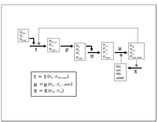
activity.  M  =  [ Glu   Lac   Allo   cAMP ] T  is the vector of metabolites (Glu = glucose,  Lac = lactose, Allo = allolactose, cAMP = cyclic adenosine monophosphate).  The GRN  for the lac operon model using the representation of Fig 1 is shown in Fig 3. The first  equation in [1] would look like this:  G ZYA  G I  G CRP  dR ZYA,o /dt  dR _I,o /dt  dR _CRP,o /dt t ₁₁ t ₂₂ t ₃₃ 0 0 0 0 0 0 =  ­  R ZYA,o  R I,o  R CRP,o r ₁₁ r ₂₂ r ₃₃ 0 0 0 0 0 0 ­  R ZYA,o  R I,o  R CRP,o d ₁₁ d ₂₂ d ₃₃ 0 0 0 0 0 0 G ZYA  G I  G CRP  dR ZYA,o /dt  dR _I,o /dt  dR _CRP,o /dt t ₁₁ t ₂₂ t ₃₃ 0 0 0 0 0 0 t ₁₁ t ₂₂ t ₃₃ 0 0 0 0 0 0 =  ­  R ZYA,o  R I,o  R CRP,o r ₁₁ r ₂₂ r ₃₃ 0 0 0 0 0 0 r ₁₁ r ₂₂ r ₃₃ 0 0 0 0 0 0 ­  R ZYA,o  R I,o  R CRP,o d ₁₁ d ₂₂ d ₃₃ 0 0 0 0 0 0 d ₁₁ d ₂₂ d ₃₃ 0 0 0 0 0 0  [2] 

where t11 would be a function of PI and PCRP.cAMP.  For example, one could choose the 

function t11  =  (c1+c2PCRP.cAMP)/(c3+c4PI n ) to represent the activation of transcription by 

the protein complex PCRP.cAMP and inhibition by the tetrameric repressor PI (the n and ci’s 

are constant parameters; n should be greater than 1 because of the tetrameric complex of  PI).

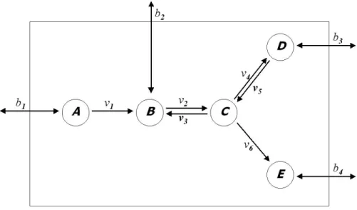
t r s m G ZYA  G _I  G CRP  _R  ZYA,o  R I,o  R CRP,o  R _Z  R Y  R I,  R CRP  P _Z,o  P _Y,o  P I,o  P _CRP,o  P _4Z  P _Ym  P 4I  P CRP.cAMP  Glu  Lac  Allo  cAMP p t = t (P 4I , P CRP.cAMP ) 

m = m (P Zo , P Io , cAMP) 

p = p (P 4Z , P Ym ) 

Figure 3.  The Lac Operon in accordance with the scheme shown in Fig 1.  See text for 

New mathematical models and reviews on the lac operon have appeared  recently. 2­4  Yildirim and Mackey 2 used delay differential equations to account for the  transcriptional and translational steps that are missing in their model.  An earlier detailed  kinetic model was proposed and analyzed by Wong, Gladney and Keasling. 1  Recently,  Vilar, Guet, and Leibler 4 used a 4­variable model that captures many of the essential  dynamics of the lac operon.  Note that the Vilar­Guet­Leibler model is essentially a three­  variable model.  The bistability exhibited by the model was used as the explanation for  the ON­OFF behavior of the lac operon.  At the single­cell level, the operon is either ON or OFF  (all­or­nothing induction)  as shown in the recent experimental report of Ozbudak et al. 3  These authors exploited the  positive feedback loop between the permease (y) and the inducer (x), and used the  following mathematical model to represent the positive feedback loop:

tydy/dt = a( 1/[1+R/Ro]) – y  [3]

txdx/dt = by – x 

where  R/RT  =  1/[1 + (x/xo) n ] 

and R = concentration of active LacI, Ro = initial concentration of active LacI, RT = total 

concentration of LacI tetramers, xo = initial concentration of LacY (permease), and the 

rest of the symbols are parameters.   The parameter n allows consideration of the fact that  the repressor is a tetramer.  This simple model generates bistability in which the all­or­  nothing transition is associated with a saddle­node bifurcation.  The simple set of  equations above was useful in guiding the authors’ experiments in showing ON­OFF

behavior as well exploring the phase diagram (coordinates of which are the variables x  and y, for example) for bistable and monostable regions.  The lac operon illustrates several important points in modeling GRNs.  Although  the operon structure is not a general property of all genomes, one can expect that genomic  DNA sequence organization affects the dynamics of the GRN;  this is primarily due to  co­expression of genes found in the same transcriptional units or co­regulation of genes  by transcription factors that recognize promoter regions having similar regulatory  sequences.  Another lesson from the lac operon is that abstraction of the complex GRN  may be sufficient to understand the behavior of the system.  This abstraction was  facilitated by prior knowledge of the influence of network topology on dynamical  behavior, e.g. bistability arising from positive feedback loops. 8  A discussion on how  network structure alone influences system behavior is provided in the penultimate section  of this chapter.  HIERARCHIES OF GRN MODELS: FROM PROBABILISTIC GRAPHS TO  DETERMINISTIC MODELS  The general representation of GRNs in Fig 1 considers groups of molecules  according to their chemical classes (DNA, RNA, proteins, metabolites) whose  “interactions” merely encode the broad concepts of transcription, post­transcriptional  processing, translation and post­translational modifications.  Depending on the nature of

available experimental information, specific models of gene regulatory networks can be  constructed at various levels of detail.  Networks, in general, are described by their graphical structures.  A graph is  basically a set of ‘nodes’ and a set of ‘edges’, the latter being the representations of the  interactions or associations among nodes.  Progressively more detailed mechanistic  information can be added to a graph as they become available.  At one extreme of the  spectrum of models, the nodes in the graph could be just a set of genes (and no other  kinds of objects), with certain pairs of genes linked by undirected edges if these pairs are  known to “interact” or are “associated” in some way.  Sometimes the nodes could be  proteins and the edges represent physical interactions.  Because of the correspondence  between proteins and genes (albeit not generally one­to­one), protein­protein interaction  networks may imply some underlying GRN structure.  In general, nodes in a graph can be  defined according to the level of detail that is sufficient to describe a particular feature,  function or behavior of the system.  For example, the nodes in Fig 1 represent various  classes of molecules.  A node could also represent a subnetwork or module with specific  cellular function.  An edge of a graph is assigned a direction if there is information on causality, i.e.  that one node affects the state of the other.  A directed edge can be further characterized  as either “activating” or “inhibiting”.  As more quantitative data are available, it may be  possible to identify the “strength” of an edge.  For dynamic models, the strength of an  edge would, for example, require identification of rate expressions as functions of the  states of the nodes.  At this point, a dynamic model encoded in deterministic differential  equations is possible.  Finally, at the other extreme in the spectrum of GRN models,

microscopic details of the interactions between individual molecular species are known  and molecular dynamic simulations are possible.  As the example of the lac operon illustrates, abstract models involving differential  equations that do not necessarily reflect the detailed mechanism are sometimes used  when the goal is primarily to explore possible system dynamics arising from the structure  of the network.  Associated with the process of ‘abstraction’ is the problem of reducing  the network into a smaller set of ‘modules’ and their interactions.  Modules can range  from individual molecules or genes, to a set of genes or proteins, or to functional  subnetworks with definable cellular functions.  Similar ideas have been discussed  recently by Vilar et al. 4 in their work on the lac operon.  The lac operon is an example of  a well­defined small model system in which a considerable amount of biological  knowledge and mechanistic understanding have already accumulated so that refined  mathematical modeling can be carried out.  Many other focused models and  corresponding mathematical model formalisms have been reviewed recently by de Jong. 9  In contrast, constructing the network graph of gene interactions from large­scale gene  expression measurements is just beginning and is, at times, controversial.  Since this field  has been reviewed 10­13 recently only a brief account is given below. 

High­throughput gene expression measurements using DNA microarrays provide  global snapshots of the dynamics of gene networks at the RNA level.  Expression data are  intrinsically noisy and conclusions derived from them are probabilistic in nature.  Furthermore, the mRNA levels are averages from cell populations.  Gene network  reconstruction from microarray data also suffers from the so­called ‘dimensionality  problem’ 11 because the number of genes is much greater than the number of microarray

experiments.  Statistical analysis of gene expression data usually employ clustering  methods to find genes with similar expression patterns across time series or across  different experimental conditions (e.g. see Refs. 14­15).  The assumption is that clustered  or co­expressed genes are somehow co­regulated or perhaps share similar functions.  The  results of clustering in terms of GRN modeling could therefore be a coarse­grain network  composed of modules (nodes), each module representing a set of genes with similar  functions. Graphical models that combine probability theory and graph theory are suitable  frameworks for inferring GRNs from gene expression data. 10, 16  In general, these  graphical models are probability models for multivariate random variables whose  independence structure can be represented by a conditional independence graph.  Recently, Friedman 10 reviewed the field of probabilistic graphical models for gene  networks, including Bayesian networks.  In a Bayesian network, the nodes represent  random variables (e.g. genes and their expression levels) while the edges show  conditional dependence relations.  Husmeier 17­18 has also reviewed the applications of  Bayesian networks to microarray data.  Bayesian networks were first applied to the  problem of reverse engineering of GRNs from microarray expression data by Friedman et  al., 19 Pe’er et al., 20 and Hartemink et al. 21  Other examples of graphical models employing  various statistical methods are discussed by Wang, Myklebost and Hovig. 16 

Zak et al. 22 have argued that inferring the GRN structure from expression data  alone is impossible.  However, promising results come from more recent work showing  that properly designed perturbation experiments do permit network reconstruction (see  Refs. 12, 13, 18, 23­25).  Two papers 23­24 extended ideas from metabolic control analysis

to suggest perturbation experiments designed to determine the direction and strengths of  interactions between genes.  Also, Gardner et al. 25 used systematic perturbations  combined with least­squares regression to infer the gene network topology and weights of  interactions.  In general, the issues encountered during the creation of a GRN graph are similar  to those faced when designing a pathway or interaction database.  These issues will be  discussed in more detail in the section on ‘pathway ontology’ below.  An extensive  discussion on this ontology is provided because it is a crucial stepping stone for future  projects concerned with the extraction of GRN models from pathways databases.  Pathways databases are relatively recent developments in bioinformatics.  These  databases are built from more elementary databases and it is important to be aware of the  many heterogeneous bioinformatics resources available, most of them on the internet.  Thus, a brief guide is given next.  A GUIDE TO DATABASES AND KNOWLEDGEBASES ON THE INTERNET  The field of bioinformatics has naturally arisen to cope with the deluge of data  generated by high­throughput technologies in genomics, transcriptomics, proteomics, and  other –omics.  These data are organized into databases (DBs) and knowledgebases (KBs),  many of which are publicly available on the internet.  Comprehensive and realistic  modeling of GRNs should tap into the information contained in these DBs and KBs.  Thus, it is expected that the next generation of modelers will have to be sufficiently

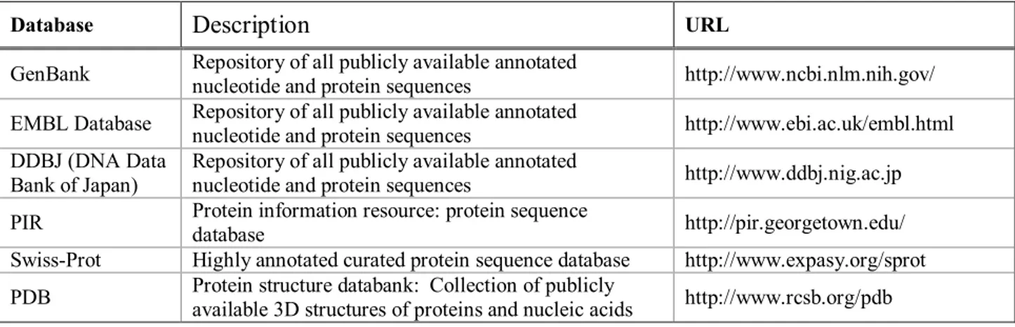
aware of bioinformatics resources.  It is for this reason that an overview of the major  bioinformatics DBs and KBs is provided here, although their utility for modeling GRNs  may not be direct and obvious at this time.  It was alluded to in the discussion of the lac  operon that understanding the operon structure of the genomic DNA was necessary to  understand the dynamics of the network.  In general, relating genome organization to  GRN dynamics is a very difficult and still a very much open problem.  This section  begins with genomic sequence databases in anticipation of their future use in helping  predict GRN structures; a specific example would be that of finding regulatory sequences  where transcription factors bind thereby linking one gene product to the transcription of  another gene.  To date, the genomes of more than 150 organisms have been sequenced, and  many more sequencing projects are currently going on or planned.  Publicly available  DNA sequence data as well as functional and structural data on proteins are accumulating  at an exponential rate, virtually doubling every year.  The major sequence and structure  repositories which are regularly updated are listed in Table 1.

Table 1. Major sequence and structure repositories 

Database  Description  URL 

GenBank  Repository of all publicly available annotated  nucleotide and protein sequences  http://www.ncbi.nlm.nih.gov/  EMBL Database  Repository of all publicly available annotated  nucleotide and protein sequences  http://www.ebi.ac.uk/embl.html  DDBJ (DNA Data  Bank of Japan)  Repository of all publicly available annotated  nucleotide and protein sequences  http://www.ddbj.nig.ac.jp  PIR  Protein information resource: protein sequence  database  http://pir.georgetown.edu/ 

Swiss­Prot  Highly annotated curated protein sequence database  http://www.expasy.org/sprot  PDB  Protein structure databank:  Collection of publicly 

available 3D structures of proteins and nucleic acids  http://www.rcsb.org/pdb 

Table 2. Protein sequence and structure property databases 

Database  Description  URL 

eMOTIF  Protein sequence motif database  http://motif.stanford.edu/emotif  InterPro  Integrated resource of protein families, domains  http://www.ebi.ac.uk/interpro  iProClass  Integrated protein classification database  http://pir.georgetown.edu/iproclass/  ProDom  Protein domain families  http://www.toulouse.inra.fr/prodom.html  CDD  Conserved domain database: covers protein domain 

information from Pfam, SMART and COG databases 

http://www.ncbi.nlm.nih.gov/Structure/cdd  /cdd.shtml 

CATH  Protein structure classification database  http://www.biochem.ucl.ac.uk/bsm/cath/  CE  Repository of  3D Protein structure alignments  http://cl.sdsc.edu/ce.html 

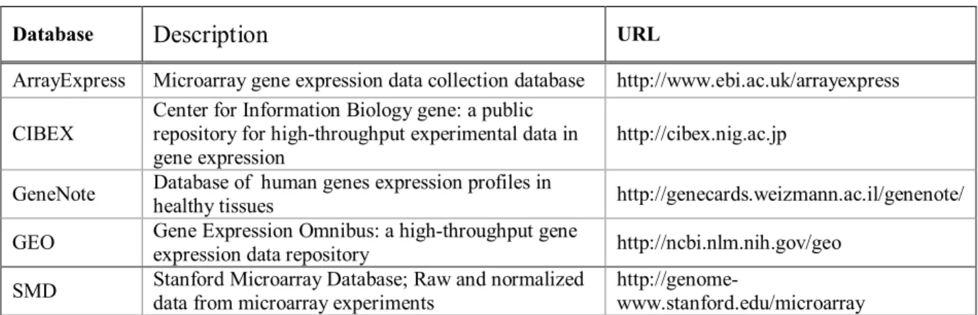
The partners of the International Nucleotide Sequence Databases (INSD), namely  GenBank, EMBL and DDBJ, share their nucleic acid sequence data for a comprehensive  coverage of all available genome information.  Swiss­Prot is a manually curated protein  sequence database with a high level annotation of protein function and protein  modifications, including links to property, structure and pathways databases.  PIR is  similar to Swiss­Prot, with the former providing some options for sequence analysis.  Recently, UniProt Knowledgebase (http://www.uniprot.org) was established with the aim  of unifying and linking protein databases with cross­references and query options.  Some of the major protein sequence and structure property databases are listed in  Table 2.  Although there are many more general or specialized property databases  available, 26 the list given in Table 2 is a good start for exploring protein property  databases.  Table 3 gives a list of gene expression repositories.  It is very difficult for one person to keep up with the rapidly increasing number of  genomics, proteomics, and interactomics and metabolomics databases, let alone their  intended usage. 26  To alleviate this problem, an increasing number of integrated database  retrieval and analysis systems tools are being developed for the purpose of data  management, acquisition, integration, visualization, sharing and analysis.  Table 4 lists  promising examples of these tools, which are regularly maintained and updated.  GeneCards is an integrated database of human genes, genomic maps, proteins, and  diseases, with software that retrieves, combines, searches, and displays human genome  information.  GenomNet is of particular interest since its analytical tools are

Table 3. Gene expression databases 

Database  Description  URL 

ArrayExpress  Microarray gene expression data collection database  http://www.ebi.ac.uk/arrayexpress  CIBEX  Center for Information Biology gene: a public  repository for high­throughput experimental data in  gene expression  http://cibex.nig.ac.jp  GeneNote  Database of  human genes expression profiles in  healthy tissues  http://genecards.weizmann.ac.il/genenote/  GEO  Gene Expression Omnibus: a high­throughput gene 

expression data repository  http://ncbi.nlm.nih.gov/geo  SMD  Stanford Microarray Database; Raw and normalized  data from microarray experiments  http://genome­  www.stanford.edu/microarray  Table 4. Integrated database retrieval and analysis systems 

Database  Description  URL 

GeneCards  Database of human genes, proteins and their involvement 

in  diseases  http://bioinfo.weizmann.ac.il/cards 

GenomeNet  Network of database and computational services for 

genome research  http://www.genome.ad.jp/ 

NCBI  Retrieval system for searching several linked databases  http://www.ncbi.nlm.nih.gov  PathPort/ToolBus  Collection of web­services for gene prediction and  multiple sequence alignment, along with visualization  tools  https://www.vbi.vt.edu/pathport  SRS­EBI  Integration system for both data retrieval and applications  for data analysis  http://srs.ebi.ac.uk

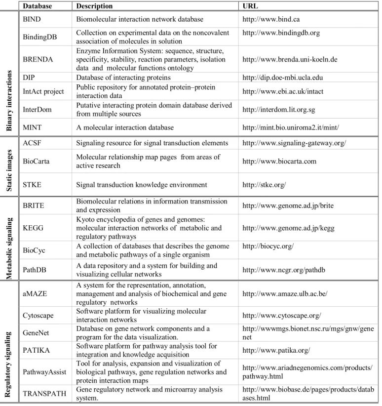
tightly linked with the KEGG pathways database (discussed in the next section).  ToolBus  comprises several data analysis software platforms such as multiple sequence alignment,  phylogenetic trees, generic XML viewer, pathways and microarray analysis, which are  linked to each other as well as to major databases.  SRS and NCBI serve as general data  retrieval portals as well as to provide links to specific analysis tools.  PATHWAYS DATABASES AND PLATFORMS  Along with recent advances in genomics and proteomics, requirements for  analysis, expansion and visualization of cell signaling, GRNs and protein­protein  interaction maps are leading to the development of data representation and integration  tools.  Pathways databases can be classified into four groups according to their  interactome data content and representation as listed in Table 5.  Only those websites that  are regularly maintained are included in the list.  The first group of databases represents  binary interaction databases.  BIND, DIP, and MINT document experimentally  determined protein­protein interactions from peer­reviewed literature or from other  curated databases.  BIND and MINT store experimental conditions used to observe the  interaction, chemical action, kinetics and other information linked to the original research  articles. 

Static image databases are very good sources of pathway diagrams which provide  a broad introductory view of cell regulatory pathways along with good reviews and links.

Table 5.  Pathways databases and platforms 

Database  Description  URL 

BIND  Biomolecular interaction network database  http://www.bind.ca  BindingDB  Collection on experimental data on the noncovalent  association of molecules in solution  http://www.bindingdb.org  BRENDA  Enzyme Information System: sequence, structure,  specificity, stability, reaction parameters, isolation  data  and  molecular functions ontology  http://www.brenda.uni­koeln.de  DIP  Database of interacting proteins  http://dip.doe­mbi.ucla.edu  IntAct project  Public repository for annotated protein–protein  interaction data  http://www.ebi.ac.uk/intact  InterDom  Putative interacting protein domain database derived  from multiple sources  http://interdom.lit.org.sg  Bi n ar y  i n te r a c ti on s 

MINT  A molecular interaction database  http://mint.bio.uniroma2.it/mint/  ACSF  Signaling resource for signal transduction elements  http://www.signaling­gateway.org/  BioCarta  Molecular relationship map pages  from areas of  active research  http://www.biocarta.com  S tati c  im age s 

STKE  Signal transduction knowledge environment  http://stke.org/  BRITE  Biomolecular relations in information transmission  and expression  http://www.genome.ad.jp/brite  KEGG  Kyoto encyclopedia of genes and genomes:  molecular interaction networks of  metabolic and  regulatory pathways  http://www.genome.ad.jp/kegg  BioCyc  A collection of databases that describes the genome  and metabolic pathways of a single organism  http://biocyc.org/  M e tab o li c  s ign al in g   PathDB  A data repository and a system for building and  visualizing cellular networks  http://www.ncgr.org/pathdb  aMAZE  A system for the representation, annotation,  management and analysis of biochemical and gene  regulatory  networks  http://www.amaze.ulb.ac.be/  Cytoscape  Software platform for visualizing molecular  interaction networks  http://www.cytoscape.org/  GeneNet  Database on gene network components and a  program for the data visualization.  http://wwwmgs.bionet.nsc.ru/mgs/gnw/gene  net  PATIKA  Software platform for pathway analysis tool for  integration and knowledge acquisition  http://www.patika.org/  PathwayAssist  Tool for analysis, expansion and visualization of  biological pathways, gene regulation networks and  protein interaction maps  http://www.ariadnegenomics.com/products/  pathway.html  R e gu lato r y  s ign al in g   TRANSPATH  Gene regulatory network and microarray analysis  system.  http://www.biobase.de/pages/products/datab  ases.html

ACSF, STKE and Biocarta are comprehensive knowledgebases on signal transduction  pathways and other regulatory networks. 

Metabolic signaling databases contain detailed information on metabolic  pathways.  These DBs have well established data structures but have non­uniform  ontologies.  BioCyc is a collection of pathway/genome databases for many bacteria and  up to 14 species of other organisms.  Enzyme catalyzed reactions, or the gene that 

encodes that enzyme or the structures of chemical compounds in pathways and reactions,  can be displayed by BioCyc ontology based software for a given biochemical pathway.  In addition BioCyc supports computational tools for simulation of metabolic pathways.  KEGG is a frequently (daily) updated group of databases for the computerized  knowledge representation of molecular interaction networks in metabolism, genetic  information processing, environmental information processing, cellular processes and  human diseases.  The data objects in the KEGG databases are all represented as graphs  and various computational methods for analyzing and manipulating these graphs are  available.  The fourth category of the DBs and software platforms listed in Table 5 is  concerned with regulatory signaling networks.  GeneNet, aMAZE and PATIKA possess  very similar ontologies for representing and analyzing molecular interactions and cellular  processes.  PATIKA and GeneNet provide graphical user interfaces for illustrating 

signaling networks . The aMAZE tool called LightBench 27 allows users to browse  information stored in the database which covers chemical reactions, genes and enzymes  involved in metabolic pathways, and transcriptional regulation.  Another aMAZE tool 

Both GeneNet and PATIKA are composed of a server­side with a database and  client­side.  In addition to its database components, a PATIKA client­side editor software  provides an integrated, multi­user environment for visualizing, entering and manipulating  networks of cellular events independent of an additional web­browser.  Cytoscape and PathwayAssist are similar software tools for automated analysis,  integration and visualization of protein interaction maps.  In these tools, automated  methods for mining PubMed and other public literature databases are incorporated to  facilitate the discovery of possible interactions or associations between genes or proteins.  ONTOLOGIES FOR GRN MODELING  Bioinformatics is now moving towards the direction of creating tools, languages  and software for the integration of heterogeneous biological data and their analysis at the  level of cellular systems and beyond.  This direction requires establishing appropriate  ‘ontologies’ to annotate the various parts and events occurring in the system.  An  ontology is a set of controlled and unambiguous vocabulary for describing objects and  concepts. 28  Current Gene, Interaction, and Pathway Ontologies  At the genome level, the Gene Ontology TM (GO) Consortium  (http://www.geneontology.org) introduced a comprehensive bio­ontology that is aimed to 

“molecular function”, “biological process” and “cellular component” searchable through  the AmiGO tool (http://www.godatabase.org).  Note that these three concepts (especially  the concept of “biological process”) can be interpreted in terms of memberships of genes  in cellular pathways; hence GO can be considered as part of a pathway ontology. 

A conventional approach for representing cellular pathways is the use of static  diagrams such as those found in the websites of ACSF, BioCarta and STKE  (see Table  5).  These diagrams are often not reusable, and the pathway representations are far from  being uniform and consistent among different websites; this is because the various  representations carry implicit conventions rather than explicit rules as required by formal  ontologies.  Because pathways are basically composed of components and steps or  processes, the development of interaction databases is a logical first step (see sample  databases in Table 5­Binary interactions).  These databases provide diverse amount of  binary interaction data, which could then be used for building networks.  Among the cellular pathways, metabolic pathways are generally more detailed  and structured because of more advanced knowledge about metabolism in cells (see  Table 5­Metabolic signaling).  In all of these databases, the proteins are classified  according to the Enzyme Commission list of enzymes (EC numbers).  These metabolic  DBs have strict ontologies which are focused on protein activities relevant to metabolic  pathways.  Due to a detailed knowledgebase and ontology, metabolic pathways are quite  amenable to kinetic modeling and computer simulations. 29

Whole­cell modeling platforms  There are a number of whole­cell modeling and simulation software environments  (e.g. Virtual Cell, E­Cell and CellWare) with their specific ontologies.  Virtual Cell 30  provides a subcellular localization­based visual environment for modeling cellular events.  The ontology is mainly based on a single mechanistic physiological model that encodes  the general structure and function of a cellular event such as release of calcium and its  effects on the cell.  In Virtual Cell a cell is considered as distinct geometrical sub­  domains containing specific cellular components with known concentration.  This model  allows users to proceed through Virtual Cell simulation tools.  Even though Virtual Cell  has some applications relevant to GRNs (e.g. Ran­protein dependent transport of proteins  between cytosol and nucleus), the platform may have difficulties in modeling events that  occur only in one cellular compartment with unknown molecular concentrations.  E­Cell 31­32 is a generic software platform for visualization, modeling and  simulation of whole cell events.  E­Cell provides several graphical interfaces for user  definable models of certain cellular states.  A cell model can be constructed with three  classes of objects (entities): substances, genes and reaction rules.  The E­Cell ontology  shares several similarities with the PATIKA ontology which is discussed in the next  section.  CellWare 33 is a multi­algorithmic software platform for modeling and simulation  of cellular events.  It has several toolboxes including tools for user­dependent model  description, definition and construction using a graph editor. A simulation toolbox  contains various simulation algorithms and interfaces from which a user can choose.

Ontology for modeling multi­scale and incomplete networks  The current state of our knowledge on cellular regulatory pathways is still  fragmented, incomplete, and uncertain in many respects despite accumulating data.  A  pathway ontology should be able to represent available information even when it is  incomplete, thus allowing incremental construction of pathways.  In addition, the  ontology must have the flexibility for continuous modification of data without  compromising the integrity of the network being built.  Therefore the ontology must  describe integrity rules of the pathway data, enabling the construction of a robust model  of the system.  A data integrity rule should state that for every instance of a bioentity (see  below), a primary key with an accession number such as (SwissProt ID) must exist and  be unique.  The seamless integration of various hierarchies of detail or scale is a key  problem in modeling and in the representation of complex systems like a cell.  Pathway visualization using diagrams or graphs facilitates the creation of a  mathematical model of a GRN.  An efficient visualization scheme is generated when an  ontology uses intuitive images.  The ontology should offer ways to reduce the complexity  of the information at some stage of the modeling process.  The discussion in the next sub­section focuses on an ontology that is suitable for  modeling incomplete information and abstractions of varying levels of complexity.  This  ontology has been recently implemented in a pathway database tool named PATIKA  (Pathway Analysis Tool for Integration and Knowledge Acquisition). 34­35  The Pathway  Database System (PDS) developed by Krishnamurthy et al. 36 shares several basic  similarities with PATIKA in terms of database organization and visualization.  As in  PATIKA, PDS provides tools for modeling, storing, analyzing, visualizing and querying

biological pathways.  However, PDS does not define a formal ontology for GRNs but  instead follows the rules of KEGG metabolic pathway ontology and uses KEGG data.  An ontology for cellular processes  States and bioentities.  Components of a GRN are macromolecules (e.g. DNAs,  RNAs or proteins), small molecules (e.g. ions, GTP or ATP), or physical events (e.g.  heat, radiation or mechanical stress).  Often, these players share a common synthesis  pathway and/or are chemically very similar.  For example, the p53 protein has many  states including its native, phosphorylated, nuclear or MDM2­bound forms.  These states  are represented as nodes in the network graph, while maintaining their biological or  chemical groupings under a common bioentity.  Transitions.  A transition represents a cellular event and each is represented as a  separate node in the graph (see Fig 4 and Fig 5).  A state may go through a certain  transition, may be produced by a transition, or may affect a transition as being an  activator or inhibitor.  When a transition occurs, all of its products are generated.

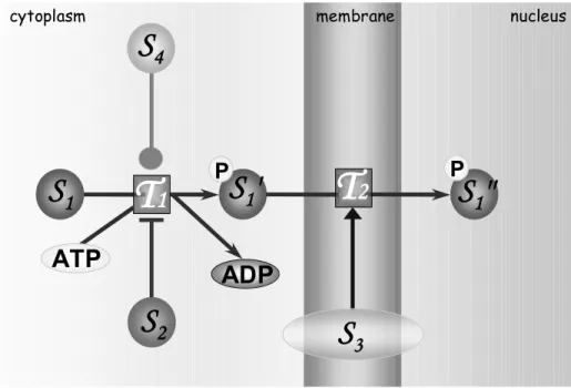
Figure 4.  An illustration of the basic features of the PATIKA ontology.  States, 

transitions, and interactions are represented by circles, rectangles and lines, respectively.  The bioentity “S1” has 3 states (namely, S1, S1' and S1'' ) located in two distinct 

subcellular compartments (cytoplasm and nucleus) which are separated by a third  compartment, the nuclear membrane.  S1 and S1' are both in the cytoplasm.  S1 is  phosphorylated through transition T1 giving rise to a new state, the phosphorylated S1'. 

S1' is translocated to the nucleus through transition T2 and becomes S1''.  T1 has two  effector states, S2 (inhibitor) and S4 (unspecified effect).  T2 has an activator type of  effector (S3) representing, for example, the nuclear pore complex.

T

1

S

'

T

2

S

S

''

ATP

S

S

ADP

S

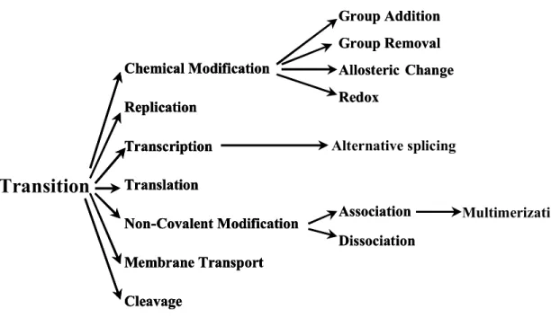
Figure 5.  Proposed tree structure used to classify transitions in the PATIKA ontology.  If  the nature of a transition can not be defined in the existing ontology, it can be considered  as generic transition to be defined and added in the ontology. 

Transition 

Compartments.  Transitions also include transport of molecules between cell  compartments. The set of transitions that a state can be involved in is strictly related to its  compartment; accordingly a change in the compartment means a change in the state’s  information context.  The state’s compartment is a part of the ontology.  As the  compartments and their vicinity are cell­type dependent, compartmental structure can be  modeled as part of the ontology.  Cell membranes create an additional complexity since  not only can a molecule be located completely inside the membrane, it may also  communicate with both sides of the membrane as part of the events involved in adjacent  compartments.  So membranes are considered as separate compartments in the ontology.  Molecular complexes.  In biological systems, molecules often form complexes in  order to perform certain tasks (Fig 6).  Each member of a molecular complex can be  considered as a new state of its associated bioentity.  The intrinsic specific binding  relations affect the function of a molecular complex.  Therefore these binding relations  must be represented in the model ontology.  Moreover, members of a molecular complex  may independently participate in different transitions; thus one should be able to address  each member individually (Fig 6).  In addition, a molecular complex may contain  members from neighboring compartments (e.g. receptor­ligand complexes).  Abstractions.  Various levels of abstractions are employed in the analysis of  complex cellular events.  A set of transitions can be described as a single ‘process’ (e.g.  the MAPK pathway), and a set of related processes may be classified under one ‘cellular  mechanism’ (e.g. apoptosis).  Some explicit examples of abstractions are shown in Fig 6.  In cases where it is not identified which state among a set of states constitutes the

substrate or effector of a transition, or where target transition of an effector is unclear, we  may need to abstract these states (or transitions) as a single state (or transition) to  represent the available information despite its incomplete nature.  The PATIKA pathway ontology  A pathway is an abstraction of a certain biological event and is the primary  abstraction in the PATIKA ontology. 35  The context of this abstraction can change from a  single molecule–molecule interaction to a complete network of all the interactions in a  cell.  In PATIKA, a pathway is represented by a pathway graph, which is a compound  graph. 37  A pathway graph is defined by an interaction graph G = (V , E) along with a  number of rules on the topology; V is the union of a finite set of states Vs and a finite set 

of transitions Vt .  E is the union of interactions of five sets: substrate edges Es, product 

edges Ep, activator effector edges Ea, inhibitor effector edges Ei, effector of unknown type 

edges Eu, and each directed edge belonging to either Vt × Vs (for product edges) or to Vs × 

Vt (for remaining interaction edge types).  Every state has a defined type: DNA, RNA, 

protein, small molecule or physical factor.  States are also associated with a specific  compartment.  Identical states in different compartments are considered as separate  states.  States of the same biological origin and/or similar chemical structure are grouped  under a biological entity or simply bioentity that act as state and transition connectivity  data holders in PATIKA.

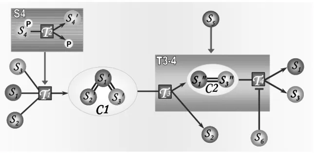
Figure 6.  A pathway containing two abstractions and a molecular complex C1 

(composed of three states S1, S2 and S3).  Super­state S4 is an example of an abstraction in  which the state S4­P or S4’ may act as an activator of transition T2.  S5 leads to the 

dissociation of complex C1 acting on either before or after the dissociation of S2. 

Therefore S5 may be an activator of either T3 or T4 ;  thus, S5 is illustrated as the activator  of super­transition T3­4.

T

T

S

S

S

S

S

'

S

'

T

T

S

S

S

T

T

S

S

C2

S

T

T

S

'

_S

_'

S

'

S

'

S

'

_S

_S

_'

_'

S

'

S

'

C1

S

'

S

'

_S

_S

_'

_'

S

'

S

'

S

'

S

'

_S

_S

_'

_'

S

'

S

'

C1

S

S

S

''

S

S

''

S

'

S

'

S

'

S

'

C1

S

S

S

''

S

S

''

S

'

S

'

C1

S

S

S

''

S

S

''

S

S

S

''

S

S

''

Every transition must be affiliated with at least one substrate and one product  edge.  It may have an arbitrary number of effectors, a combination of which defines the  exact behavior for the transition. Transitions are classified according to the tree shown in  Fig 5.  A transition is not associated with a specific compartment; instead, its  compartment is determined by its interacting states.  Different types of molecules (e.g.  protein, DNA and RNA) have distinct user interfaces for easier visual discrimination in  PATIKA.  Compartmental information is also modeled.  PATIKA also implements  collaborative construction and modification to existing regulatory signaling data on the  database.  Therefore PATIKA maintains version numbers as part of the ID of each graph  object.  Thus it is possible that while a user is working on a PATIKA graph locally, others  might change the topology and/or properties of states and transitions in the PATIKA  database.  EXTRACTING MODELS FROM PATHWAYS DATABASES  A clear pathway ontology, as discussed in the previous section, will allow  systematic methods for extracting GRN models from the interactions stored in a  pathways database.  The specific model would, of course, depend on the particular  biological question being asked.  Here, a brief example is given of how a model is  extracted from a network of interactions taken from some of the databases listed in Table  5.   The work of Aguda and Tang 38 on the G1 checkpoint of the cell cycle is used as an  example.  A cell cycle checkpoint is a surveillance mechanism that arrests or slows down  cell cycle progression if something goes wrong, e.g. DNA damage.  The significance of

elucidating the control mechanism of the G1 checkpoint lies in the observation that many  human cancers are associated with nonfunctional G1 checkpoints.  A qualitative network of the G1­S transition is shown in Fig 7.  The network was  generated by integrating information from the published literature, including sequence  analysis of upstream regulatory regions of genes that are targeted by the E2F  transcription factor family.  Aguda and Tang 38 were interested in finding a minimal  subnetwork that is sufficient to explain the switching behavior of the G1 checkpoint.  The  key step towards finding this subnetwork was the hypothesis that there is a core set of  interactions with an intrinsic instability that ultimately generates a switching behavior  (see refs. 38 and 39 for details; network stability analysis is discussed in the next section).  Experimentally, the activity of cyclin E/CDK2 is used as a marker for the entry into the S  phase of the cell cycle.  Hence, this minimal set of interactions must include  cyclinE/CDK2.  In the network graph shown in Fig 7, the arrows are interpreted as “activation”  and the hammerheads as “inhibition”.  From this qualitative network, a network stability  analysis (discussed in the next section) pointed to a core mechanism involving cyclin  E/CDK2, Cdc25A, p27Kip1 and their interactions.  These interactions involve two  coupled positive feedback loops, namely, between the pair (Cdk2/Cyclin E, Cdc25A) and  the pair (Cdk2/Cyclin E, p27).  This core mechanism was then used as the basis for a  more detailed mechanistic model.  The dynamics of the model was coded into differential  equations and solved in a computer.  The computer simulations reproduced the  experimentally observed qualitative behavior of the G1 checkpoint. 38

A discussion of the mathematical and computational tools already available for  the analysis of GRN models is given in the next section.  Most of the models extracted  from pathways databases are expected to be qualitative and incomplete in nature; hence  the discussion focuses on qualitative network structures and how these structures  influence the capacity of the system to exhibit certain dynamical behavior.

ORC  Cdc6  MCMs  Cdc7  E2F DP  pRb  Cyclin­D/cdk4  _{Cyclin­A/cdk2}  Cdk2/Cyclin­E  Cdc25A  p27  GFs  Figure 7.  A qualitative network involving key interactions in the G1­S transition of the  mammalian cell cycle.  Solid lines are post­translational modifications or protein­protein  interactions.  Dashed arrows are transcriptional steps.  Arrows mean “activation”, and  hammerheads mean “inhibition”.  GFs = growth factors, cdk = cyclin­dependent kinase,  pRb = retinoblastoma protein, ORC = origin recognition complex.

PATHWAY AND DYNAMIC ANALYSIS TOOLS FOR GRNS  Selection of the appropriate network analysis tool depends on the questions being  asked and the scale or size of the network being considered.  Questions of robustness of  the entire system against perturbations require more consideration of global network  properties and less of the attributes of individual processes or reactions.  Questions  focusing on particular phenomena, such as the switching behavior of a particular set of  genes, may require more attention to the local network details involving these genes.  How the global and local network properties interplay to produce local or system­level  behavior is an important problem that requires multi­scale analysis, both in time and  space.  In this section, a brief account is given on global network properties, how large  networks can be analyzed or reduced by identifying recurring network motifs and  extreme pathways, and how topology or network structure alone may already determine a  network’s stability and its capacity to exhibit certain dynamical behavior.  The goal of  this section is not to provide a comprehensive review of the aforementioned topics (as  they are quite broad and recent reviews will be cited) but, instead, to point out particular  directions of analysis of a GRN model once it has been constructed.  Global network properties  Considering the very large number of interacting genes, proteins and other  molecules in a living cell, one would first like to ask questions about global features and  properties of the entire network.  How connected are the nodes in the network, and what  is the mean path length between any two nodes?  Are there clusters of interactions so that

one may subdivide the network into modules?  How robust is the system to perturbations  – i.e. are there redundant pathways that could take over if a pathway is cut off, so that the  system’s function is still intact?  In general, the aim is to identify global network  topological features that affect system function or behavior independent of the details of  the individual nodes or interactions.  There had been various attempts at searching for  quantifiable structural features of metabolic networks, signaling networks, and GRNs  (see Ref. 40 for a review).  Some basic network descriptors are the degree distribution,  the path length distribution, and the clustering coefficient. 

The degree distribution P(k) is the probability that a node is linked to k other  nodes.  The P(k) of random networks exhibits a Poisson distribution whereas that of  scale­free networks approximates a power law of the form P(k) ~k ­g .  An interesting  suggestion is that most cellular networks approximate a scale­free topology 41­42 with an  exponent γ between 2 and 3. 43­44  The interpretation of this suggestion is not clear.  The path length distribution of a network tells us how far nodes are from each  other.  Scale­free networks are ‘ultra­small’ since they have an average path length of the  order log(log N), where N is the number of nodes.  Random networks are ‘small’ because  their mean path length is of the order log N . 43­44 

The clustering coefficient of a particular node A of a network is defined by C(A)  = 2n(A) / (k(A)(k(A)­1)), where k(A) is the number of neighbors of A, and n(A) is the  number of connections between the neighbors of A. 40  The average clustering coefficient  characterizes the tendency of a network to form node clusters, and is a measure of the  network's modularity.  The average clustering coefficient of most real networks is larger

than that of same­size random networks. 45  Cellular networks have a high average  clustering coefficient, which indicates a highly modular structure. 46­47  Recurring network motifs  One approach that could simplify the analysis of a large network is to look for  recurring motifs which are subgraphs that are over­represented in the network. 48­51 The  motivation is that each motif can be analyzed separately for its intrinsic properties, and  the original network may be reduced to a set of motif interactions.  Recent analysis 48  show that three­node feed­forward motifs are abundant in transcriptional regulatory  networks and neural networks, while  four­node feedback loops are characteristic of  electric circuits, but not of biological networks.  Remarkable evolutionary conservation  of motifs 52 and convergent evolution toward the same motif types in transcriptional  regulatory networks of diverse species 53­54 show that motifs are indeed significant  biologically.  Identifying pathway channels in networks: extreme pathway analysis  Another way of coping with large networks involves breaking down the network  into channels through which distinct processes are carried out.  Clarke 55 developed a  formalism called ‘Stoichiometric Network Analysis’ and was the first to show that all  steady­state fluxes are found in a convex set called the ‘current cone’; furthermore, he  showed that each cone has a certain number of edge vectors that can be uniquely  determined from the stoichiometric matrix.  Clarke referred to the pathways  corresponding to the edge vectors as ‘extreme currents’; alternatively, these are called