Noise analysis of geometrically complex mechanical structures using the analogy between electrical circuits and mechanical systems

Noise analysis of geometrically complex mechanical structures using the analogy

between electrical circuits and mechanical systems

G. G. Yaralioglu, and A. Atalar

Citation: Review of Scientific Instruments 70, 2379 (1999); View online: https://doi.org/10.1063/1.1149766

View Table of Contents: http://aip.scitation.org/toc/rsi/70/5

Random fluctuations of displacement or velocity in mechanical systems can be calculated by using the analogy between electrical circuits and mechanical systems. The fluctuation-dissipation theorem expresses the relation between the generalized mechanical admittance and the noise in velocity. Similarly, correlation of mechanical noise can be calculated by using the generalized Nyquist theorem which states that the current noise correlation between two ports in an electrical circuit is dictated by the real part of the transadmittance. In this article, we will present the determination of the mechanical transadmittance and we will use the mechanical transadmittance to calculate the noise correlation on geometrically complex structures where it is not possible to approximate the noise by using the simple harmonic oscillator model. We will apply our method to atomic force microscope cantilevers by means of finite element method tools. The application of the noise correlation calculation method to rectangular cantilever beams shows some interesting results. We found that on the resonance frequencies, the correlation coefficient takes values 1~full correlation! and21 ~anti-correlation! along the cantilever axis depending on the mode shapes of the structure. © 1999 American Institute of Physics.@S0034-6748~99!04005-8#

I. INTRODUCTION

Random vibrations of mechanical parts set the funda-mental limit on the minimal detectable displacement in many precision displacement measuring devices like the atomic force microscope ~AFM!, laser interferometric gravitational wave detectors, accelerometers, etc. Similar to the series voltage noise of a resistor in an electrical circuit, the source of random vibrations is the thermal agitation. To determine the merit of a displacement sensing system, it is crucial to understand this noise source and calculate the amplitude of the random vibrations.

The resolution of an AFM system which uses an optical detection method is determined by the thermal noise of the cantilever. In an optical AFM system, the cantilever is illu-minated by a laser beam and the reflected beam from the cantilever is detected by a photodetector. Since the laser in-tegrates the mechanical noise within its beam, the correlation of noise plays an important role in the output noise.

Thermal noise of an AFM cantilever has been inten-sively studied.1–5In most of the earlier work, the cantilever has been modeled by a simple harmonic oscillator and the noise of the free end has been calculated by employing the equipartition theorem.6 However, the output noise calcula-tion of the optical AFM system using the simple harmonic oscillator model assumes that the noise within the laser illu-mination is fully correlated. As we will show in Sec. IV, this is a good approximation to predict the output noise for simple AFM cantilevers since the noise correlation varies slowly at the free end. However, for geometrically complex structures like interdigital cantilevers7,8which are composed

of two sets of interleaving fingers, the noise correlation be-tween fingers should be calculated for an accurate analysis of the noise performance.

In this work, we will present a method for the calcula-tion of noise and noise correlacalcula-tion for geometrically complex mechanical structures. The structure may be made up of dif-ferent materials or may have difdif-ferent loss coefficients in different parts of the structure. For the noise calculation, we will employ the analogy between electrical circuits and me-chanical systems. First, electrical noise equations will be pre-sented. We will repeat the result of the fluctuation-dissipation theorem9,10for the calculation of noise at a single point, then present the calculation of noise correlation be-tween two points on the mechanical structure. For the me-chanical response calculations, we will use the finite element method~FEM!. Depending on the FEM meshing of the me-chanical structure, we will define the noise correlation matrix corresponding to the mechanical structure.

We will also define the noise correlation coefficient which can be used to estimate the degree of noise correlation between different parts of the structure.

II. ELECTRICAL NOISE EQUATIONS

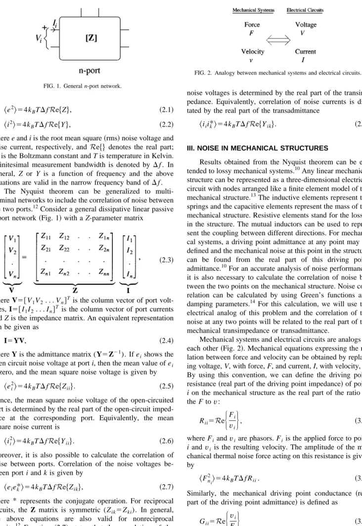
In dissipative linear electrical systems, thermal or Johnson noise was characterized by Nyquist11 in 1928. The thermal noise of a two terminal network can be represented by a series voltage noise source, e, or by a shunt current noise source, i, as determined by the Nyquist theorem. The mean values of the source phasors are zero,

^

&

^

&

and the mean square noise voltage or noise current is deter-mined by the real part of the impedance~Z! or the admittance ~Y! seen between the terminals

a!_{Electronic mail: goksenin@ee.bilkent.edu.tr}

2379

^

&

^

&

where e and i is the root mean square~rms! noise voltage and noise current, respectively, and Re$% denotes the real part;

k_B is the Boltzmann constant and T is temperature in Kelvin. Infinitesimal measurement bandwidth is denoted by D f . In general, Z or Y is a function of frequency and the above equations are valid in the narrow frequency band of D f .

The Nyquist theorem can be generalized to multi-terminal networks to include the correlation of noise between the two ports.12Consider a general dissipative linear passive

n-port network~Fig. 1! with a Z-parameter matrix

~2.3!

where V5@V1V2. . . Vn#T is the column vector of port

volt-ages, I5@I1I2. . . In#T is the column vector of port currents

and Z is the impedance matrix. An equivalent representation can be given as

I5YV, ~2.4!

where Y is the admittance matrix (Y5Z21). If ei shows the

open circuit noise voltage at port i, then the mean value of ei

is zero, and the mean square noise voltage is given by

^

&

Hence, the mean square noise voltage of the open-circuited port is determined by the real part of the open-circuit imped-ance at the corresponding port. Equivalently, the mean square noise current is

^

&

Moreover, it is also possible to calculate the correlation of noise between ports. Correlation of the noise voltages be-tween port i and k is given by

^

&

where * represents the conjugate operation. For reciprocal circuits, the Z matrix is symmetric (Zik5Zki). In general,

the above equations are also valid for nonreciprocal circuits.12 Equation ~2.7! states that the correlation of the

noise voltages is determined by the real part of the transim-pedance. Equivalently, correlation of noise currents is dic-tated by the real part of the transadmittance

^

&

III. NOISE IN MECHANICAL STRUCTURES

Results obtained from the Nyquist theorem can be ex-tended to lossy mechanical systems.10Any linear mechanical structure can be represented as a three-dimensional electrical circuit with nodes arranged like a finite element model of the mechanical structure.13 The inductive elements represent the springs and the capacitive elements represent the mass of the mechanical structure. Resistive elements stand for the losses in the structure. The mutual inductors can be used to repre-sent the coupling between different directions. For mechani-cal systems, a driving point admittance at any point may be defined and the mechanical noise at this point in the structure can be found from the real part of this driving point admittance.10For an accurate analysis of noise performance, it is also necessary to calculate the correlation of noise be-tween the two points on the mechanical structure. Noise cor-relation can be calculated by using Green’s functions and damping parameters.14 For this calculation, we will use the electrical analog of this problem and the correlation of the noise at any two points will be related to the real part of the mechanical transimpedance or transadmittance.

Mechanical systems and electrical circuits are analogs of each other~Fig. 2!. Mechanical equations expressing the re-lation between force and velocity can be obtained by replac-ing voltage, V, with force, F, and current, I, with velocity,v.

By using this convention, we can define the driving point resistance~real part of the driving point impedance! of point

i on the mechanical structure as the real part of the ratio of

the F tov: Rii5Re

H

Fi

vi

J

, ~3.1!

where Fiandviare phasors. Fi is the applied force to point

i and vi is the resulting velocity. The amplitude of the

me-chanical thermal noise force acting on this resistance is given by

^

i

2

_&

BTD f Rii. ~3.2!

Similarly, the mechanical driving point conductance ~real part of the driving point admittance! is defined as

G_ii5Re

H

J

~3.3!

FIG. 1. General n-port network.

FIG. 2. Analogy between mechanical systems and electrical circuits.

volves applying a sinusoidal force to a specific point i and measuring the velocity of the same point. If there is no loss in the mechanical structure, the phase difference between the force phasor and the velocity phasor will be 90° or 290°. Hence, Eqs. ~3.2! and ~3.4! will give zero noise. Similarly, we can find the transadmittance between two points by ap-plying a sinusoidal force to the point i and measuring the velocity of the other point k. Transconductance is given by

Gik5Re

H

vk

Fi

J

. ~3.5!

By using the mechanical analog of Eq.~2.8!, the correlation of the velocity noise between two points is given by

^

&

It is customary to use the rms displacement noise, rather than the noise in velocity. We can easily derive noise equa-tions for displacement, u, from Eqs. ~3.4! and ~3.6!. Since velocity is the derivative of displacement, the Nyquist rela-tion for the displacement noise is

^

_&

H

J

k is

^

&

H

J

where Im$% denotes the imaginary part and v52pf is the

radial measurement frequency. For displacement we can de-fine a noise correlation matrix, N, where the diagonal ele-ments show the mean square absolute displacement noise at point i and the off-diagonal elements are the correlation of displacement noise between points i and k:

Nik5

^

&

The noise correlation matrix is symmetric for reciprocal sys-tems.

IV. APPLICATION OF THE METHOD: CANTILEVER BEAM

Cantilever beams are widely used in atomic force mi-croscopy. The deflection of the cantilever is monitored to measure the atomic forces. Noise analysis of the cantilever beam is especially important for AFM where the ultimate resolution of the system is determined by the thermal me-chanical noise of the cantilever.

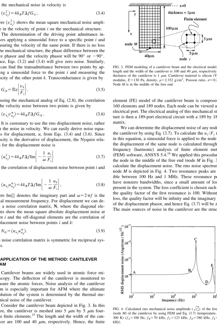
Consider the cantilever beam depicted in Fig. 3. In this figure, the cantilever is meshed into 5 mm by 5 mm four-node finite elements.15 The length and the width of the can-tilever are 100 and 40 mm, respectively. Hence, the finite

element ~FE! model of the cantilever beam is composed of 160 elements and 189 nodes. Each node can be viewed as an electrical port. The electrical analog of this mechanical struc-ture is then a 189-port electrical circuit with a 189 by 189 Z matrix.

We can determine the displacement noise of any node on the cantilever by using Eq.~3.7!. To calculate the u_i/F_iratio in this equation, a sinusoidal force is applied to the node and the displacement of the same node is calculated through the frequency ~harmonic! analysis of finite element method ~FEM! software, ANSYS 5.4.16_{We applied this procedure to}

the node in the middle of the free end~node M in Fig. 3! to calculate the displacement noise. The rms noise spectrum of node M is depicted in Fig. 4. Two resonance peaks are vis-ible between 100 Hz and 1 MHz. These resonance peaks have nonzero bandwidths, since a small amount of loss is present in the system. The loss coefficient is chosen such that the quality factor of the first resonance is 100. Without the loss, the quality factor will be infinity and the imaginary part of the displacement phasor, and hence Eq.~3.7! will be zero. The main sources of noise in the cantilever are the structure

FIG. 3. FEM modeling of a cantilever beam and the electrical model. The length and the width of the cantilever is 100 and 40mm, respectively. The thickness of the cantilever is 1mm. Cantilever material is silicon~Young modulus, E5130 Pa, density,r52.332 g/cm3_{, Poisson ratio,s50.278).} Node M is in the middle of the free end.

FIG. 4. Calculated rms mechanical noise amplitude (Azn2) of the free end

~node M! of the cantilever by using FEM and Eq. ~3.7! ~temperature, T, is

300 K! ( fA5100 Hz, fB570 kHz, fC5123 kHz, fD5380 kHz, fE5768 kHz!.

damping ~Rayleigh damping!, air damping and coupling to the bulk waves in the cantilever stand.

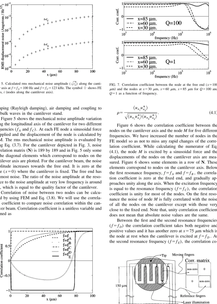
Figure 5 shows the mechanical noise amplitude variation along the longitudinal axis of the cantilever for two different frequencies ( f_A and f_C). At each FE node a sinusoidal force is applied and the displacement of the node is calculated by FEM. The rms mechanical noise amplitude is evaluated by using Eq. ~3.7!. For the cantilever depicted in Fig. 3, noise correlation matrix~N! is 189 by 189 and in Fig. 5 only some of the diagonal elements which correspond to nodes on the cantilever axis are plotted. For the cantilever beam, the noise amplitude increases towards the free end. It is zero at the node (x50) where the cantilever is fixed. The free end has the most noise. The ratio of the noise amplitude at the reso-nance to the noise amplitude at very low frequency is around 100, which is equal to the quality factor of the cantilever.

Correlation of noise between two nodes can be calcu-lated by using FEM and Eq.~3.8!. We will use the correla-tion coefficient to compare noise correlacorrela-tion within the can-tilever beam. Correlation coefficient is a unitless variable and defined as

r5

^

&

A

^

&^

&

. ~4.1!

Figure 6 shows the correlation coefficient between the nodes on the cantilever axis and the node M for five different frequencies. We have increased the number of nodes in the FE model so as not to miss any rapid changes of the corre-lation coefficient. While calculating the numerator of Eq. ~4.1!, the node M is excited by a sinusoidal force and the displacements of the nodes on the cantilever axis are mea-sured. Figure 6 shows some elements in a row of N. These elements correspond to nodes on the cantilever axis. Below the first resonance frequency, f5 fA and f5 fB, the

correla-tion coefficient is zero at the fixed end, and gradually ap-proaches unity along the axis. When the excitation frequency is equal to the resonance frequency ( f5 fC), the correlation

coefficient is unity for most of the nodes. On the first reso-nance the noise of node M is fully correlated with the noise of all the nodes on the cantilever except with those very close to the fixed end. Note that, unity correlation coefficient does not mean that absolute noise values are the same.

Between the first and the second resonance frequencies ( f5 f_D) the correlation coefficient takes both negative and positive values and it has another zero at x575mm which is the node at rest when the cantilever is excited at f5 fD. At

the second resonance frequency ( f5 fE), the correlation

co-FIG. 5. Calculated rms mechanical noise amplitude (Azn

2_{) along the} canti-lever axis at f5 fA5100 Hz and f 5 fC5123 kHz. The symbol L shows FE nodes, i~nodes along the cantilever axis!.

FIG. 6. Correlation coefficient between the nodes along the cantilever axis and the node at the middle of the node M.

FIG. 7. Correlation coefficient between the node at the free end (x5100

mm! and the nodes at x530mm, x560mm, x585mm for Q5100 and Q51 as a function of frequency.

FIG. 8. Interdigital cantilever and the form of correlation matrix.

efficient is 21 between the fixed end and the node at rest (x578 mm!, which means that this part of the axis is anti-correlated with the free end, whereas other nodes ~between the node M and the node at rest! are fully correlated with the free end.

The correlation coefficient can also be calculated as a function of frequency. Figure 7 shows the correlation coef-ficients between the three different points on the axis and the node M for two different quality factors. For high Q systems, the correlation coefficient is very weakly dependent on Q. Only when the quality factor is very low is a significant change observed. We note that, below the first resonance, the correlation coefficient is almost independent of loss.

Interdigital ~ID! cantilevers7,8 are new interferometric deflection detection sensors for atomic force microscopy. An ID cantilever is composed of two sets of interleaving fingers ~reference fingers, moving fingers! to form an optical diffrac-tion grating as depicted in Fig. 8. Such gratings when illu-minated by a laser beam reflect incidence light into many orders. The intensities of the orders depend on the relative displacement of the fingers. If a photodetector is used to detect the order intensity, the output current from the detec-tor gives the cantilever deflection. The total noise at the de-tector output is determined by integrating the mechanical noise within the illuminated area on the cantilever. For the accurate evaluation of the output noise, the noise correlation between fingers should be calculated.

For the ID cantilever, the correlation matrix has the form depicted in Fig. 8 if the FEM nodes are arranged properly. Off-diagonal sub-matrices are zero since there is no me-chanical coupling between alternate fingers; for example, the correlation between nodes A~on reference fingers! and D ~on moving fingers! is zero. In this section, we will present the correlation coefficient calculation between two reference fin-gers, specifically between nodes A, B and C as depicted in Fig. 8.

There is a close relationship between resonance mode shapes and the correlation coefficient. Figure 9 shows the mode shapes of the ID cantilever at the first longitudinal resonances. There are four longitudinal resonances between 0 and 300 kHz. The length of the fingers is 70 mm. The cantilever material is silicon and the thickness is 1mm. Fig-ure 10 shows the correlation coefficient between nodes A

and B and between nodes A and C. The resonances reveal themselves as peaks in Fig. 10. At f1all fingers move up and

down at the same time as depicted in Fig. 9, hence at this frequency, noise displacements at nodes A, B and C are posi-tively correlated. At f2, B and C move in the opposite

di-rection of A. Hence correlation coefficients, rAB, rAC, are

negative. At f3, A and B move in the same direction which

gives positive correlation, whereas the motions of A and C are in the opposite direction as depicted in Fig. 9, hencerAC

is negative. At f₄, the situation is reversed;r_ABis negative andr_ACis positive.

ACKNOWLEDGMENTS

The authors would like to thank Professor B. A. Auld and Dr. E. Gustafson of Stanford University for valuable discussions.

1_{Y. Martin, C. C. Williams, and H. K. Wickramasinghe, J. Appl. Phys. 61,} 4723~1987!.

2

N. Osakabe, K. Harada, M. I. Lutwyche, H. Kasai, and A. Tonomura, Appl. Phys. Lett. 70, 940~1997!.

3_{A. Garcia-Valenzue, J. Appl. Phys. 82, 985~1997!.}

4_{A. Garcia-Valenzue and J. Villatoro, J. Appl. Phys. 84, 58~1988!.} 5

M. V. Salapaka, H. S. Bergh, J. Lai, A. Majumdar, and E. McFarland, J. Appl. Phys. 81, 2480~1997!.

6_{K. Huang, Statistical Mechanics~Wiley, New York, 1987!.}

7_{S. R. Manalis, S. C. Minne, A. Atalar, and C. F. Quate, Appl. Phys. Lett.}

69, 3944~1996!.

8

G. G. Yaralioglu, A. Atalar, S. R. Manalis, and C. F. Quate, J. Appl. Phys.

83, 7405~1998!.

9_{P. R. Saulson, Phys. Rev. D 42, 2437~1990!.}

10_{H. B. Callen and T. A. Welton, Phys. Rev. 83, 34~1951!.} 11

H. Nyquist, Phys. Rev. 32, 110~1928!. 12

R. Q. Twiss, J. Appl. Phys. 26, 599~1955!.

13_{S. Seely, Dynamic Systems Analysis~Reinhold, New York, 1964!.} 14_{N. Nakagawa, B. A. Auld, E. Gustafson, and M. M. Fejer, Rev. Sci.}

Instrum. 68, 3553~1997!. 15

A four-node elastic shell element~SHELL63! of ANSYS is used to con-struct the finite element model for the cantilever.

16_{ANSYS, Inc., 201 Johnson Road, Houston, PA 15342-0065.} FIG. 9. Mode shapes of the fingers at different resonance frequencies. The

length of the reference part is 150mm. Finger length is 70mm. Arrows indicate the direction of motion. Dotted lines show the undeformed shape of the ID cantilever.

FIG. 10. Calculated correlation coefficients between nodes A and B and between nodes A and C.