An Integrated Model for Visualizing Biclusters from Gene Expression Data and PPI Networks

An Integrated Model for Visualizing Biclusters from Gene

Expression Data and PPI Networks

Ahmet Emre Alada ˘g

Computer Engineering Kadir Has University Istanbul, 34083, Turkey

emre.aladag@stu.khas.edu.tr

Cesim Erten

Computer Engineering Kadir Has University Istanbul, 34083, Turkey

cesim@khas.edu.tr

Melih Sözdinler

melih.sozdinler@boun.edu.tr

ABSTRACT

We provide a model to integrate the visualization of biclusters ex-tracted from gene expresion data and the underlying PPI networks. Such an integration conveys the biologically relevant interconnec-tion between these two structures inferred from biological experi-ments. We model the reliabilities of the structures using directed graphs with vertex and edge weights. The resulting graphs are drawn using appropriate weighted modifications of the algorithms necessary for the layered drawings of directed graphs. We provide applications of the proposed visualization model on the S.cerevisiae dataset.

Categories and Subject Descriptors

H.5 [Information Interfaces and Presentation]: Miscellaneous; H.1 [Information Systems]: Models and Principles

General Terms

Design, Algorithms

Keywords

Bicluster, PPI network, Visualization

1.

INTRODUCTION

In a gene expression data matrix the rows correspond to the genes and the columns correspond to the conditions such as time points or environmental conditions of interest. Each entry of the matrix is a real number that represents the expression level of a gene un-der a certain condition. Several techniques have been suggested to analyze gene expression data to gather useful biological corre-lations. Biclustering is one such technique that refers to the pro-cess of extracting submatrices of genes and conditions exhibiting “significant” correlation across both the rows and the columns of the data matrix. In more general settings its first appearance has usually been attributed to Hartigan under the name direct cluster-ing[15]. Almost thirty years later the technique has been intro-duced to the field of gene expression analysis, first by Cheng and

Permission to make digital or hard copies of all or part of this work for personal or classroom use is granted without fee provided that copies are not made or distributed for profit or commercial advantage and that copies bear this notice and the full citation on the first page. To copy otherwise, to republish, to post on servers or to redistribute to lists, requires prior specific permission and/or a fee.

ISB’10February 15-17, 2010, Calicut, India.

Copyright 2010 ACM 978-1-60558-722-6/10/02 ...$10.00.

Church [7]. Since then several methods have been suggested for the problem; see [20] for a survey. Another common structure that en-ables an understanding of cellular mechanisms and processes is that of protein interactions. As proteins rarely act as isolated species, but rather form a close association with partner proteins for some specific biological activity, it is necessary to analyze these interac-tions which globally give rise to protein-protein interaction (PPI) networks. There is usually a natural interconnection between the information contained within gene expression data and the PPI net-works [17]. The validity of extracted high-level structures as bi-clusters is usually cross-checked via low-level biological data such as in the form of protein interactions [12, 22]. Conversely, to im-prove the accuracy and the coverage of protein interactions it is usually necessary to integrate complementary data sources includ-ing gene expression [19]. In order to reflect this interconnection and the recently growing need for integrated inference and analysis methods, it is crucial to provide visualization models that integrate the high-level structures arising from expression data and the rela-tively low-level experimentally inferred PPI networks. Reliability is a major concern for both biclusters and the protein interactions. The biclustering algorithms are usually based on well known sta-tistical data mining techniques and thus should be cross validated with previously known biological results. Similarly the PPI net-works are generated using various experimental approaches. As the experimental techniques suffer from noise and systematic bi-ases several computational methods are employed for improving confidence. Nevertheless in both biclustering and the protein in-teractions data there are techniques to assign a confidence value to the resulting inferences. A faithful visualization of these inferred structures should embed the confidence values in the visualization model.

We provide a model that integrates the visualization of biclusters and the underlying PPI networks. Besides the obvious role in con-veying biologically relevant interconnection, such an integration is also important as a visualization aid. Large graphs such as the PPI networks are usually visualized using an appropriate form of clus-tered graph visualization, where the clusters are formed using some graph-theoretical measures. With the proposed integration such a clustering is indirectly achieved using natural context-based mea-sures. The reliabilities of the inferred structures are modelled using weights. The main layout paradigm used in the visualization model is the Sugiyama-style layered drawings. The resulting weighted graphs are laid out using appropriately modified algorithms neces-sary for this layout style.

2.

PREVIOUS WORK

Several methods and tools for the visualization and analysis of PPI networks have previously been proposed [5, 11, 16, 24].

Usu-ally the visualization of the network is done as a whole and various analysis options are provided within the tools. One such widely used visualization tool is Cytoscape [24]. It supports many of the layout paradigms suggested for graph visualization in literature. Its main advantage is that it is extendible with plugins such as Gene-Pro [28]. GeneGene-Pro provides a cluster-centric visualization of PPI networks with features similar to our proposed model. However the visualization model lacks the important concept of reliability. The directional information inherent in the structures is also not represented as a result of the choice of the layout algorithm. In SpringScape the main layout is based on a spring embedder [11]. It is yet another tool with similar concepts of integrating differ-ent biological information from multiple data sources such as gene expression and PPI networks. This integration is realized on the same view which leads to cluttered visualization. The absence of a clustering paradigm, be it contextual or graph theoretical, adds another complication to readability of the visualized graphs. Sim-ilar to GenePro the reliability factor has no affect on the produced visualizations.

On the other hand a number of tools and methods have also been suggested for visualization and analysis of biclusters. Bi-cat [2], Click and Expander [25] are tools that can be employed both for biclustering the data in the expression matrix and also for basic visualizations of the output biclusters. Heatmaps and gene versus condition plots constitute the employed visualization tech-niques. Bicoverlapper is a bicluster visualization tool that uses a force directed layout [23]. It supports many visualization function-alities. However, the tool itself is complicated and slow because of a straightforward implementation of the force directed layout com-putations. Furthermore it has no components to integrate various data sources. BiGGEsTS [14] is another tool aimed at visual anal-ysis of biclusters. The employed visualization techniques include parallel coordinate, heatmap, and graph visualizations. Enrichment ratio calculations based on p-values can be considered as a measure of what we call reliability. However as far as the graph visualiza-tions are concerned, the representavisualiza-tions of these measures are only limited to visual clues such as color intensity. The suggested vi-sualization methods do not take into account the reliability values while producing the final graph layout itself. Moreover there is not a general model to integrate the visualization of a bicluster with that of biologically relevant data. Such an integration is only provided via the construction of a graph of enriched GO terms per bicluster. In more general settings starting with Sugiyama et al [26] the layered drawing paradigm has received considerable attention in graph drawing literature; see [3] for a survey. Although weighted versions of some of the steps involved in the layered drawing paradigm such as layer assignment [13] or vertex orderings within layers [6] have previously been suggested, none of them presents a compre-hensive approach covering all the major steps.

3.

VISUALIZATION MODEL

3.1

Modelling Integration and Reliability

To convey the interconnection between the bicluster structures and the protein interactions we provide a two-level visualization model; see Figure 1. The first level is the central view represen-tation which shows the high-level relationships between biclusters, the bicluster graph. Each vertex in the graph corresponds to a bi-cluster that is extracted from a given gene expression data matrix using some specific biclustering algorithm. The second level is the detailed peripheral view which shows the possible low-level rela-tionships in the form of protein interactions between pairs of genes

inside each bicluster from the central view. The vertices and edges are assigned weights appropriately in the constructed graphs. The vertex and edge weights assigned in both bicluster graphs in the central view and the subgraphs of the PPI network in the peripheral view are employed in the layout phase so that the visualization can capture the reliability inherent in the structures. Additionally to en-hance visual understanding the vertices are drawn in sizes, and the edges are drawn with thicknesses proportional to their weights.

3.1.1

Peripheral View: PPI Subgraphs

It is the subgraph of the global PPI network that is defined on the genes contained within the bicluster. Each gene corresponds to a vertex and there exists an edge (u, v) with weight w(u, v) if the underlying PPI network contains an interaction from gene u to gene v. The weight w(u, v) represents the reliability of the inter-action. Suthram et al. define a confidence score between 0 and 1 for the protein interactions [27]. We normalize these scores to in-teger values and obtain the corresponding edge weight. The PPI networks of the selected sets of biclusters constitute the peripheral view of the visualization.

3.1.2

Central View: Bicluster Graph

The vertices of the bicluster graph are weighted and each weight represents the quality (reliability) of the corresponding bicluster. We use two alternative scoring functions for this weight assignment to reflect the quality. One is to evaluate a bicluster in terms of its H-value (mean squared residue) [7] and assign the weight accordingly. Assume a bicluster as a submatrix with I rows and J columns. The residue R of an entry at the ith_{row and the j}th_{column is defined}

as,

RI,J(i, j) = ai,j− aIj− aiJ+ aIJ,

where aiJ is the mean of row i, aIjis the mean of column j and

aIJis the mean of the submatrix. H-value is then defined as,

H(I, J) = 1 |I||J| X i=0,j=0 (RI,J(i, j) 2 ).

With this measure the lower the H-value of a bicluster is, the more “correlated” the data values are. Therefore the weight of a vertex u, denoted with w(u), is the inverse of the H-value of the sub-matrix corresponding to the bicluster denoted with u. As a sec-ond alternative for the vertex weights we propose to use contextual interpretations gathered from the biclusters. The Gene Ontology (GO) Consortium has published curated gene-attribute association lists for several organisms [9]. For instance, each gene of Yeast belongs to one of 13 main categories including Energy Production, Amino Acid Metabolism, Cellular Fate. Given a set of genes it is straightforward to find its enrichment ratio which corresponds to the ratio of the number of genes associated with the dominant at-tribute (functional category) in the whole set to the size of the set. Each vertex weight w(u) is equal to the enrichment ratio of the bicluster corresponding to u in this case.

We propose two alternatives for the edges of the bicluster graph as well. In the first alternative every pair of vertices u, v are con-nected with an undirected edge with weight w(u, v) equal to the number of shared genes in the biclusters corresponding to u, v. Next the edges not satisfying a minimum weight threshold are re-moved from the graph. Such a visualization is especially preferable if the biclustering algorithm provides overlapping biclusters and the emphasis of the relationship between biclusters is on the degree of these overlaps. Analogous to the vertex weighting alternatives, the second alternative scheme for edge weights is again context-based.

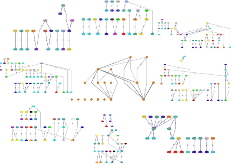
Figure 1: Snapshot of the proposed visualization model with the central and peripheral views. Bicluster graph is at the center. Biclusters of interest are clicked and the PPI network corresponding to them are laid out on the peripheral view. Colors of vertices in the peripheral view indicate the different functional categories. The directions of edges are naturally downward. Only the upward edge directions are indicated with arrows to reduce the clutter in the visualization.

A directed edge from u to v is created if there exists a considerable number of reliable protein interactions from the set of genes inside the bicluster u to the set of genes inside the bicluster v. The weight assignment is defined as

w(u, v) = X

∀gi∈u,gj∈v

w(gi, gj).

Here w(gi, gj) is the weight of the edge between the genes gi, gjin

the underlying global PPI network and it corresponds basically to the reliability of the interaction. Both alternatives are designed so as to provide clues on how to modify an unsatisfactory biclustering at hand. If a bicluster is to be expanded the most similar biclusters which are the graph-theoretically closest ones are to be considered first. The difference between these alternative schemes is that the similarity in the former is captured in essence by the degree of over-laps which in turn is a property of the employed biclustering algo-rithm, whereas the latter provides such clues after a context-based and integrated interpretation of the underlying structures.

3.2

Layout Algorithm

We employ the layered drawing paradigm for both graph types. Proposed by Sugiyama et al., it is the layout style where a directed graph is embedded in layers in such a way that the directional flow of the graph is clearly visible and certain aesthetic criteria are achieved. Attributed to these constraints, there are usually three main steps involved: Cycle Removal, Layer Assignment, and Or-dering within Layers. For the first step the usual goal is to remove cycles by reversing the minimum number of edges in the graph. Once an acyclic graph is achieved the next step assigns disjoint subsets of vertices to the layers. Several optimization goals includ-ing minimizinclud-ing the number of layers or minimizinclud-ing the number of vertices in any layer can be employed. Finally the order of the ver-tices in each layer should be assigned in such a way that the number of edge crossings in the complete layout is minimized. Almost all the interesting versions of each step is an NP-hard task. We pro-pose a weighted extension of the mentioned steps. We note that both the vertices and the edges in the graphs under consideration are weighted. Since the steps involved in the layout computation are usually related to optimizing certain criteria with regards to the

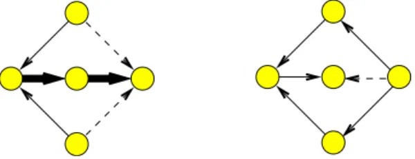
Figure 2: Left: The optimum solution to weighted FAS reverses two light edges. Right: One heavy edge reversed if weights are not considered.

edges of the graph we first modify the edge weights so as to include both the original weights of the edges and the weights of the inci-dent vertices. For the layout purposes each edge (u, v) is assigned the weight

s

w(u) × w(v)

outdeg(u) × indeg(v)× w(e(u, v))

where w(u), w(v), w(u, v) represent the original weights of the vertices and the edge, and outdeg, indeg represent the outdegree and the indegree of the vertex respectively. The contribution of the vertices is determined by the geometric mean of the contribu-tion of each vertex independently. This independent contribucontribu-tion is computed as the weight of the vertex distributed over all outgo-ing (incomoutgo-ing) edges. Given an edge-weighted directed graph, the problem now is to redefine each of the main steps of the layered drawing paradigm considering edge weights and provide appropri-ate solutions.

3.2.1

Cycle Removal

This phase is closely related to the Feedback Arc Set (FAS) prob-lem. Given a directed graph, the problem is to find the minimum size subset of edges such that when removed or reversed the graph no longer contains a cycle. The decision version is one of Karp’s 21 problems and is NP-hard [18]. For the weighted version of the problem the goal is to reverse a subset of edges such that the sum of the weights of edges in the subset is minimum. Rather than re-versing heavy edges involved in some number of cycles, it might be more beneficial for visualization purposes to reverse more light edges involved in fewer cycles; see Fig 2. Demetrescu et al. pro-vide a two phase algorithm for the weighted FAS problem [10]. The first phase consists of finding a minimum weight edge in a cycle, decrementing this weight from the weights of all the edges in the cycle, removing all edges with weight zero and repeating the whole process until no cycle remains. It is guaranteed that this initial phase produces a result that is within a ratio bounded by the length of the longest cycle in the graph from the optimum. To achieve minimality the second phase goes through the reversed edge set assigning their original directions to the edges if doing so does not introduce any cycles. We implemented this algorithm as it is simple and produces good results in practice. The only differ-ence is that in our implementation the second phase goes through the list of reversed edges after sorting them in decreasing weights so as to achieve minimality first with heavy edges.

3.2.2

Layer Assignment

Each vertex is assigned to one of k layers li,1 ≤ i ≤ k in such

a way that for every edge (u, v) we have l(u) > l(v) where l(u) indicates the layer number of u. To aid the succeeding steps, an

additional requirement is that l(u) is exactly one more than l(v) for an edge (u, v). This is achieved by introducing dummy ver-tices on edges that span more than two neighboring layers. Several optimization criteria are suggested. Minimizing the height of the drawing corresponds to producing a layout with minimum num-ber of layers. Minimizing the width of the drawing corresponds to minimizing the maximum number of vertices assigned to any layer. Minimizing number of dummy vertices achieves a minimum total edge length in the drawing. Several algorithms realizing one or more of these criteria have been suggested. We employ a lay-ering algorithm that is based on the Coffman-Graham algorithm of [8] and the longest path with promotion heuristic of [21]. Our modifications are oriented towards minimizing total weighted edge lengths while providing a compact drawing area. We first compute a lexicographical ordering π on the vertices of the graph. This or-dering in a sense is a measure of the distance to a source vertex with indegree zero. In the second phase, starting from the bottom layer the algorithm assigns a layer to each vertex each time pick-ing a new vertex with maximum π(v). When v is assigned to a layer and outdeg(v) is zero the incoming edges of v are appended to a waiting list. If there is more than one candidate vertex for the waiting list, we pick the one with the maximum sum of weights of outgoing edges to be the next one in the list. In an attempt to reduce the height of the output drawings we apply a promotion heuristic. Going through the set of vertices in no particular order the gain of promoting (moving up one layer) each vertex is tested. The pro-motion of a vertex v may require a recursive propro-motion of u, if u is directly above v. A promotion is realized if it decreases the sum of weighted edge lengths and it satisfies a prespecified maximum width. This process is repeated until no layer changes are realized.

3.2.3

Ordering within Layers

Once the layers are determined the next step is to determine the order of the vertices within each layer. The goal is to minimize the number of edge crossings in the drawing. This is usually achieved with a layer-by-layer sweep technique. Starting from the first two layers, the top layer is fixed and the bottom layer is ordered using an algorithm that minimizes crossings. Next this is applied between the second layer and the third this time keeping the second layer fixed and ordering the third, and so on until all layers are swept. The sweeping may continue in the reverse direction up and down until a desired number of crossings or iterations is reached. For the weighted version of this step, we employ the WOLF algorithm for solving the subproblem of minimizing crossings in bipartite graphs when one layer is fixed. The algorithm works on weighted bipar-tite graphs and is a 3-approximation when considering the weighted sum of crossings. In addition to this theoretical guarantee it is sim-ple and is shown to work well in practice [6].

3.2.4

Coordinate Assignment

After the order of the nodes in each layer is determined, we need to assign appropriate horizontal/vertical coordinates to each node. The desired horizontal coordinates provide edges as straight as pos-sible. We employ the method suggested in [4] as it provides linear execution time and is easy to implement. This method generates at most two edge bends per edge and tries to draw inner segments ver-tically. There are two main steps involved. In the vertical alignment step, the nodes are aligned to their median upper/lower neighbors. In the horizontal compaction step, the aligned blocks of nodes are assigned to classes providing a minimum seperation distance be-tween each class of nodes. These two steps are executed four times for each direction. After aligning these possible layouts, the actual

x-coordinate for each node is computed as the average median of the four candidates.

For the vertical coordinate assignment, we set the vertical separa-tion between a pair of layers proporsepara-tional to the density of weighted edges incident to vertices in the pair. This way, the layer corridor dense with large edge weights shall be wider to highlight the im-portance of that specific layer. On the other hand, the layer corri-dor with less cumulative edge weights shall be narrower so that no space is wasted in the y-dimension.

4.

APPLICATION ON YEAST DATASET

For our visualization application we use datasets for the organ-ism S.cerevisiae (Yeast). The source code of all the implementa-tions, the experiments and more visualization applications are pub-licly available at http://hacivat.khas.edu.tr/~cesim/ integratedviz.tar.gz. The PPI network is from [27] with 11884 interactions between 4393 genes. The biclustering results are extracted partially using the Bicat [2] and the results of [12]. Finally we obtain 13 functional categories of each of the genes in the dataset from [1].

In Figure 3, the bicluster graph in the central view has 21 ver-tices which are the biclusters from the LEB algorithm [12]. There are three graphs extracted from the peripheral view. At the PPI net-work level in the peripheral view for B3and B8, coloring of

ver-tices is not dominantly on behalf of any specific color. This implies that the bicluster fails to collect genes from the same functional cat-egory, a context-based sign that the biclusters under consideration may not semantically be relevant. This is verified by the sizes of the corresponding vertices in the bicluster graph. Furthermore the corresponding graph of B2on the peripheral view is sparse which

implies the protein interactions involving the genes in this biclus-ter do not indicate a highly connected group. Because of the large number of genes inside the biclusters B3and B8, their

correspond-ing vertices have large degrees at the central view. This makes them more general gene subsets and in fact uncorrelated. Genes in B2

actually maybe more correlated than those of B3 and B8. B3has

only three light incident edges in the central view. This may be a clue to merge B3with its more generic neighbors B15 or B8that

have appropriate H-values. For instance, H-values of B15and B8

are similar and there are fairly dense genes from the category of Cellular Organizationin both.

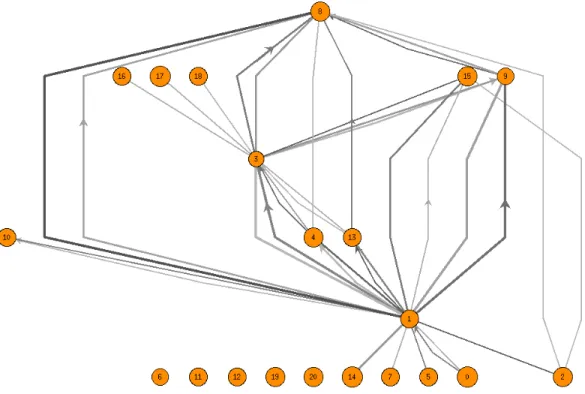
A more detailed view of B2at the peripheral view is provided in

more detail in Figure 4. When we analyze this bicluster in more de-tail, 16 of its vertices among 50 belong to the same functional cat-egory, Cellular Organization. Extending this bicluster with similar category genes might provide the ultimate bicluster as it is densely connected with fairly heavy edges in the bicluster graph, a sign of a hot spot for PPI interactions. Checking first the immediate neigh-bors in the central view for such a possible extension would provide useful. If the ultimate bicluster shows a dominant specific category according to its gene results, it is easier to check the connections of uncategorized genes just by checking relations and the H-value changes.

A detailed peripheral view of B8 is provided in Figure 6. B8

has orange circled genes colored pink which are Uncategorized. Interestingly, the pink genes seem to have interactions with the blue genes. This may be a clue that the pink uncategorized genes could be related to Translation as their blue neighbors in peripheral view are of that category.

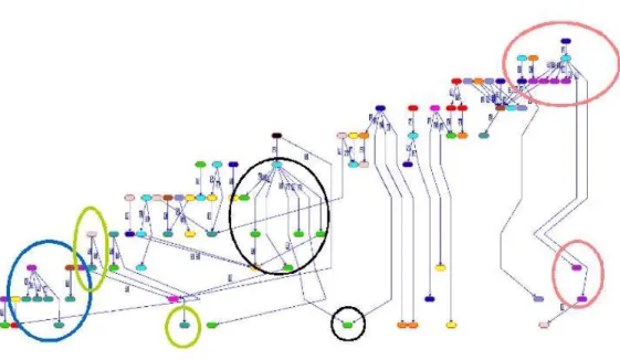
B3is presented in more detail in Figure 5. There are genes with

interactions to many different functionality genes. Green, blue, or-ange, black circles all include at least a gene interacting with

dif-ferent colored vertices, that is difdif-ferent genes. This leads to another prediction that cyan vertices inside the red circles maybe associated with Stress and Defense rather than Cellular Organization. The largest vertex in the central view is B15. This is the best

biclus-ter in biclus-terms of H-value comparison. We do not show its details in this figure but it mainly has the genes from the cyan and dark green categories, the Cellular Organization and Genome Maintenance re-spectively.

5.

CONCLUSION

We provide a visualization model that integrates different sources of biological data in the form of biclusters and protein interactions. The important concept of reliability applicable to both types of graphs is modelled using weighted graphs. The layout method em-ployed in visualizations is based on the layered drawing paradigm. Several modifications of the main steps of this paradigm are im-plemented to handle the weight generalization. Future work in-cludes extending the model with various other appropriate layout paradigms.

6.

ACKNOWLEDGEMENTS

This work is partially supported by the TUBITAK grant 109E071. Third author is supported by TUBITAK-BIDEB.

7.

REFERENCES

[1] Mips. http:

//mips.gsf.de/genre/proj/mpact/yeast. [2] S. Barkow, S. Bleuler, A. Prelic, P. Zimmermann, and

E. Zitzler. Bicat: a biclustering analysis toolbox. Bioinformatics, 22(10):1282–1283, 2006.

[3] O. Bastert and C. Matuszewski. Layered drawings of digraphs. pages 87–120, 2001.

[4] U. Brandes and B. Köpf. Fast and simple horizontal coordinate assignment. In Proc. of 9th International Symposium on Graph Drawing, pages 31–44, London, UK, 2002. Springer-Verlag.

[5] B.-J. Breitkreutz, C. Stark, and M. Tyers. Osprey: A network visualization system. Genome Biology, 3(12):1–6, 2002. [6] O. A. Çakiroglu, C. Erten, Ö. Karatas, and M. Sözdinler.

Crossing minimization in weighted bipartite graphs. Journal of Discrete Algorithms, doi:10.1016/j.jda.2008.08.003, 2008. [7] Y. Cheng and G. Church. Biclustering of expression data. In

Proc. of the 8th Int. Conf. on Intelligent Systems for Molecular Biology, pages 93–103, 2000.

[8] E. Coffman and R. L. Graham. Optimal scheduling for two-processor systems. Acta Informatica, 1:200–213, 1972. [9] Consortium. Gene ontology: tool for the unification of

biology. the gene ontology consortium. Nature Genetics, 25(1):25–29, 2000.

[10] C. Demetrescu and I. Finocchi. Combinatorial algorithms for feedback problems in directed graphs. Inf. Process. Lett., 86(3):129–136, 2003.

[11] T. M. Ebbels, B. F. Buxton, and D. T. Jones.

Springscape:visualisation of microarray and contextual bioinformatic data using spring embedding and an

´Sinformation landscapeŠ. Bioinformatics, 22(14):e99–e107, 2006.

[12] C. Erten and M. Sözdinler. Biclustering expression data based on expanding localized substructures. In Proceedings of BICoB 2009, pages 224–235, 2009.

Figure 3: S. cerevisiae. Bicluster graph from the central view in detail.

Figure 5: Bicluster 3 from the peripheral view in detail.

[13] E. Gansner, E. Koutsofios, S. North, and K. Vo. A technique for drawing directed graphs. IEEE Trans. Softw. Eng., 19(3):214–230, 1993.

[14] J. P. Gonçalves, S. C. Madeira, and A. L. Oliveira. Biggests: integrated environment for biclustering analysis of time series gene expression data. BMC Research Notes, 2(124), 2009.

[15] J. Hartigan. Direct clustering of a data matrix. Journal of the American Statistical Association, 67(337):123–129, 1972. [16] F. Iragne, M. Nikolski, B. Mathieu, D. Auber, and

D. Sherman. Proviz: protein interaction visualization and exploration. Bioinformatics, 21(2):272–274, 2005. [17] R. Jansen, D. Greenbaum, and M. Gerstein. Relating

whole-genome expression data with protein-protein interactions. Genome Research, 12(1):37–46, 2002. [18] R. M. Karp. Reducibility among combinatorial problems.

pages 85–103, 1972.

[19] X. Lin, M. Liu, and W. Chen. Assessing reliability of protein-protein interactions by integrative analysis of data in model organisms. BMC Bioinformatics, 10:S5, 2009. [20] S. Madeira and A. Oliveira. Biclustering algorithms for

biological data analysis: A survey. IEEE/ACM Trans. on Comp. Biol. and Bioinformatics, 1(1):24–45, 2004.

[21] N. Nikolov, A. Tarassov, and J. Branke. In search for efficient heuristics for minimum-width graph layering with

consideration of dummy nodes. Journal Experimental Algorithmics, 10:2.7, 2005.

[22] A. Prelic, S. Bleuler, P. Zimmermann, A. Wille, P. Buhlmann, W. Gruissem, L. Hennig, L. Thiele, and E. Zitzler. A systematic comparison and evaluation of biclustering methods for gene expression data. Bioinformatics, 22:1122–1129, 2006.

[23] R. Santamaría, R. Therón, and L. Quintales. Bicoverlapper. Bioinformatics, 24(9):1212–1213, 2008.

[24] P. Shannon, A. Markiel, O. Ozier, N. S. Baliga, J. T. Wang, D. Ramage, N. Amin, B. Schwikowski, and T. Ideker. Cytoscape: A Software Environment for Integrated Models of Biomolecular Interaction Networks. Genome Research, 13(11):2498–2504, 2003.

[25] R. Sharan, A. Maron-katz, and R. Shamir. Click and expander: A system for clustering and visualizing gene expression data. Bioinformatics, 19:1787–1799, 2003. [26] K. Sugiyama, S. Tagawa, and M. Toda. Methods for visual

understanding of hierarchical system structures. Systems, Man and Cybernetics, IEEE Transactions on,

11(2):109–125, Feb. 1981.

[27] S. Suthram, T. Shlomi, E. Ruppin, R. Sharan, and T. Ideker. A direct comparison of protein interaction confidence assignment schemes. BMC Bioinformatics, 7(1):360, 2006. [28] J. Vlasblom, S. Wu, S. Pu, M. Superina, G. Liu, C. Orsi, and

S. J. Wodak. Genepro: a cytoscape plug-in for advanced visualization and analysis of interaction networks. Bioinformatics, 22(17):2178–2179, 2006.