A collaborative system for providing routes between locations

(1)

A COLLABORATIVE SYSTEM FOR PROVIDING

ROUTES BETWEEN LOCATIONS

A THESIS

SUBMITTED TO THE DEPARTMENT OF COMPUTER ENGINEERING

AND THE INSTITUTE OF ENGINEERING AND SCIENCE OF BILKENT UNIVERSITY

IN PARTIAL FULFILLMENT OF THE REQUIREMENTS FOR THE DEGREE OF

MASTER OF SCIENCE

By K. Ali Uluğ

(2)

I certify that I have read this thesis and that in my opinion it is fully adequate, in scope and in quality, as a thesis for the degree of Master of Science.

_______________________________________ Asst. Prof. Dr. David Davenport (Advisor)

_______________________________________ Dr. Markus Schaal (Co-Advisor)

_______________________________________ Asst. Prof. Dr. H. Murat Karamüftüoğlu

_______________________________________ Asst. Prof. Dr. Savio S. H. Tse

_______________________________________ Dr. Kıvanç Dinçer

Approved for the Institute of Engineering and Science:

_______________________________________ Prof. Dr. Mehmet Baray

Director of Institute of Engineering and Science

(3)

ABSTRACT

A COLLABORATIVE SYSTEM FOR PROVIDING ROUTES

BETWEEN LOCATIONS

Kerem Ali Uluğ

M.S. in Computer Engineering Supervisor: Asst. Prof. Dr. David Davenport

Co-Supervisor: Dr. Markus Schaal June, 2008

Many systems, such as in-car GPS devices and airline company web sites, provide route information between locations. Although such systems are used widely and can provide route information successfully, users of these systems cannot contribute to the data entry process. In these systems, data is entered by the administrators and these systems cannot take advantage of the route expertise of their users.

In this work, we present a collaborative system, which provides routes between locations upon user queries. The data in the system is entered by the users of the system. We present a model which is containing locations, links between locations and relationships between locations (containment, neighborhood and intersection) in order to store the data. For the route finding purpose, we present a customized version of the A* search algorithm. This customized version, named A*CD (A* for Collaborative Data), uses heuristics for estimating the cost remaining to the target location while processing the nodes. A*CD can also provide alternative routes, exclude certain link types in the searches according to user preferences and handle the problems associated with multiple stop transportation lines. As the cost models, we use duration and financial cost.

We also present the intuitive connections concept. Even if a route does not exist between the selected locations, the system can provide a route with missing links. The gap(s) between the disconnected locations are filled by the help of the relationships between locations.

In order to evaluate the performance of the A*CD algorithm, we present automated tests. These tests show that the costs of the routes that are provided by the A*CD algorithm are close to the actual shortest routes. In order to demonstrate the intuitive connections concept, we also present manual test queries.

Keywords: Heuristic search, collaborative systems, A* search

(4)

ÖZET

MEKANLAR ARASINDA ROTALAR SUNMAK İÇİN KATILIMCI

BİR SİSTEM

Kerem Ali Uluğ

Bilgisayar Mühendisliği, Yüksek Lisans Tez Yöneticisi : Y. Doç. Dr. David Davenport

Yardımcı Tez Yöneticisi: Dr. Markus Schaal Haziran, 2008

Otomobiller için GPS cihazları ve havayolu şirketlerinin ağ siteleri gibi bir çok sistem, mekanlar arasında rota bilgileri sunmaktadır. Bu tip sistemler yaygın olarak kullanılmalarına ve rota bilgilerini doğru bir şekilde sunmalarına rağmen, kullanıcıların veri girişine izin vermemektedir. Bu tip sistemlerde tüm veri, sistem yöneticileri tarafından girilmekte ve sistemler kullanıcılarının rota tecrübelerinden faydalanamamaktadır.

Bu çalışmada, kullanıcı sorguları karşılığında mekanlar arasında rotalar sunan katılımcı bir sistem sunulmuştur. Sistemdeki veriler kullanıcılar tarafından girilmektedir. Verilerin saklanması için, mekanların, mekanlar arasındaki bağlantıların ve mekanlar arasındaki ilişkilerin (kapsama, komşuluk, kesişme) tanımlandığı bir model sunulmuştur. Rotaları bulabilmek için, A* arama algoritmasının özelleştirilmiş bir uyarlaması sunulmuştur. A*CD (A* for Collaborative Data) olarak adlandırdığımız bu uyarlama, arama esnasında mekanları işlerken, hedef mekana kalan tahmini bedeli hesaplamak için buluşsal yöntemler kullanmaktadır. Ayrıca alternatif rotalar sunmak, belli bağlantı tiplerini hariç tutmak ve çok sayıda durağa sahip taşım araçları ile ilgili sorunlara çözüm getirmek için A* arama algoritması üzerinden yapılmış değişiklikler sunulmuştur. Bedel modeli olarak seyahat süresi ve seyahat maliyeti (finansal) kullanılmaktadır.

Çalışmamızda, sezgisel bağlantılar kavramı da sunulmuştur. Seçilen mekanlar arasında bir rota bulunamaması durumunda bile, sistem eksik bağlantılara sahip bir rota dönebilmektedir. Eksik bağlantılar, mekanlar arasındaki ilişkiler yardımıyla doldurulabilmektedir.

A*CD algoritmasının performansını değerlendirmek amacıyla otomatik testler sunulmuştur. Bu testler A*CD algoritması ile bulunan rotaların bedellerinin en düşük bedelli rotaya çok yakın olduğunu göstermektedir. Sezgisel bağlantılar kavramını örneklemek için otomatik olmayan testler sunulmuştur.

Anahtar Sözcükler: Buluşsal yöntemlerle arama, katılımcı sistemler, A* arama

(5)

ACKNOWLEDGMENTS

First of all, I would like to express my gratitude to Dr. Markus Schaal due to his suggestions, and support during this research. I have learned a lot from him.

I am also indebted to Dr. David Davenport and Dr. H. Murat Karamüftüoğlu for their support and comments.

I would like to thank Dr. Savio S. H. Tse and Dr. Kıvanç Dinçer for accepting to read and review this thesis.

(6)

Chapter 1 Introduction

The best way to learn how to get from one location to another is usually to ask a person who knows the route. The route might consist of buses, taxis, sidewalks or any means of transportation. A person with an expertise on the desired route will be able to combine necessary transportation knowledge and offer the best route. On the other hand, a person has expertise on a limited number of routes. This important drawback can be eliminated by combining people’s knowledge in a collaborative system. In a collaborative system, all the data is managed by the system’s users. Wikipedia and Facebook are two popular examples of collaborative systems.

There are many systems that are providing routes between locations. In-car GPS devices provide routes by using the city road and traffic information. National train network web sites exploit train transportation information. Municipality web sites contain public bus and metro transportation information to provide routes between selected locations. Although such systems are widely used and can provide routes to the users successfully, they cannot take advantage of the route expertise of their users.

Existing systems also have another important disadvantage. They cannot take advantage of the relationships between locations. There might be different types of relationships between locations such as containment (Ankara contains Bilkent University) or neighborhood (Bilkent University and Middle East Technical University are neighbors). These relationships can be used in order to provide useful information to the user even if a route cannot be found. Consider the following scenario;

- User requests a route from Bilkent University (contained in Ankara) to Berlin Airport. - There are two airports in Istanbul, Atatürk Airport and Sabiha Gokcen Airport. - There exists a route from Bilkent University to Atatürk Airport.

- There exists a route from Sabiha Gokcen Airport to Berlin Airport. - There is no route between Bilkent University and Berlin Airport.

In this scenario, the system can conclude that two airports are connected since they are both contained in Istanbul. So, the route from Bilkent University to Atatürk Airport and also the route from Sabiha Gokcen Airport to Berlin Airport can be provided to the user together with the containment information.

1.1 Problem Definition

In this thesis, our main problem is to provide users with routes between locations, using data that has been entered by the users themselves. Gathering the data from the users is the collaborative aspect of the context. This brings a new problem associated with the quality of

(10)

CHAPTER 1. INTRODUCTION

the data. There might be missing links between locations although the links actually exist in real life. In the following scenario, a link is missing (Middle East Technical University – Bilkent University link)

- A route from Kizilay (a district in Ankara) to Bilkent University is requested - There is a route from Kizilay to Middle East Technical University

- There is no route from Kizilay to Bilkent University

- Bilkent University and Middle East Technical University are neighbors. This information has been entered by a user.

In this scenario, the system should be able to provide the route from Kizilay to Middle East Technical University and also the neighborhood information.

Also, missing links might create problems because of the duplicate information in the system. Two users might enter the same location with different names to the system. The following scenario demonstrates a situation in which there is duplicate information; two users, independent from each other, entered two locations to the system, which are both referring to the same real world location. The missing link is between the duplicate locations in this scenario.

- There are two locations named “Bilkent Engineering Building” and “Bilkent University Engineering Building” in the system. They refer to the same real world location.

- Both of these locations are contained in a location named “Bilkent University”. Data for these relationships exists in the system.

- User requests a route from a location, Kizilay (a district in Ankara) to Bilkent Engineering Building.

- There is a route from Kizilay to Bilkent University Engineering Building. - There is no route from Kizilay to Bilkent Engineering Building.

In this scenario the system should be able to provide the information to the user indicating that Bilkent Engineering Building can be reached from Kizilay by following the Kizilay to Bilkent University Engineering Building route. Since both buildings are contained in the same location, Bilkent University, the system should be able to conclude that they are connected. Such data quality problems might be handled if additional information, such as relationships between locations, exists in the system. Although there might be missing links, if the relationships have been entered properly, a solution might still be provided. We name this problem as missing links problem; there might be gaps in a route but these gaps can be filled by the help of the relationships between locations.

The provided routes’ costs should be as close as possible to the actual lowest cost routes. We don’t define a threshold for the ratio of the cost of a provided route to the actual lowest cost route. On the other hand, applying tests for a large number of location pairs and presenting the average cost ratio is in scope of this thesis.

In order to improve the running time of the algorithm, the route search should be guided by taking advantage of the data in the system (geographic coordinates, location relationships, etc.). The time and space complexity is not discussed in this work.

(11)

CHAPTER 1. INTRODUCTION

Our problem definition also contains some extensions beyond the main problem. Users should be able to request alternative routes from the system and specify either minimum duration or minimum financial cost. This choice specifies if they are interested in a fast route that will take minimum amount of time to travel or a cheap route in which they will pay less. Additionally, the system should be able to handle the problems associated with transportation lines with multiple stops.

1.2 Thesis Outline

In Chapter 2, we present details of the missing links problem and our solution to it. In Chapter 3, we give detailed descriptions of the extensions of the main problem and present solutions to them. In Chapter 4, first we present the related work for graph search algorithms and then the details of the search algorithm that we are using, A*CD (A* for Collaborative Data). In Chapter 5, we explain our implementation, mainly the modules for data entry. In Chapter 6 we present the results of our tests. We conclude the thesis with Chapter 7.

(12)

Chapter 2 Incomplete Information and Virtual Links

In this chapter, first we explain the extended unidirectional graph model for storing the data in the system. This model contains locations, links and location relationships together with their properties. Afterwards, we explain the situations in which we want to find intuitive connections for missing links, despite data problems in the base graph. Finally, we present our solution, virtual links, for the missing links problem.

2.1 A Base for Solution: Extended Unidirectional Graph

We are using a unidirectional graph as a base. A graph G is a pair (V, E). V is a set of nodes (vertices). E is a set of links (edges) between the vertices,

Each node in the graph corresponds to a location in our system. A location can be of any type, for example, it can be a country, a city, an office building or even an individual room.

Locations in our system have properties associated with them. Location type, explanation, geographical coordinates are some examples of locations’ properties. These properties are used for storing more information about a singe location.

Each edge in the graph corresponds to a unidirectional link between two locations. A link can be of any type, e.g. an international flight or a 5 minute walk. If a reverse link also exists, this is represented by another link in the system. Cycles of any length (number of nodes) are allowed in our system.

Links have several properties associated with them. Guessed duration, guessed cost (money), guessed cost currency and explanation are the link properties. We name these properties as “guessed” in order not to create a confusion with the term “estimated”, which will be used in the A*CD search algorithm.

Cost information is mandatory for links. Users should enter this information while entering a link to the system. For the financial cost, we do not request the currency rate from the users. We only take the financial cost and the currency. We maintain a currency rate table for relating all currencies with Turkish Lira so that all financial costs can be converted to Turkish Lira whenever required.

In addition to links, locations, link properties and location properties, location relationships should also be stored. There are three kinds of relationships; containment, neighborhood and intersection.

(13)

CHAPTER 2. INCOMPLETE INFORMATION AND VIRTUAL LINKS

We name two locations as parent and child if they are related with a containment relationship. We name two locations as neighbor if they are related with a neighborhood relationship. We say two locations intersect if they are related with an intersection relationship.

Figure 2.1 – An instance of the base model. Nodes have latitude, longitude and type information. Links have type, guessed duration and guessed financial cost. Node D contains node C. Nodes D and E are neighbors.

2.2 Intuitive Connections

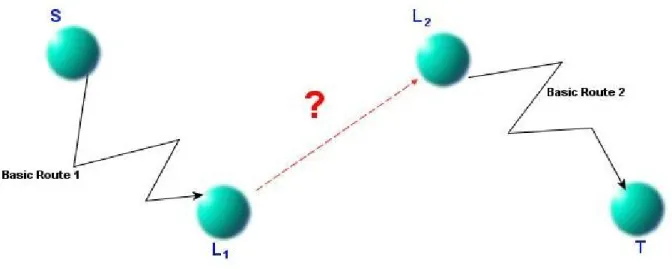
Location relationships have an important effect on the solutions provided by the system. They help provide intuitive connections so that even if a complete sequence of user entered links from the source node to the target node cannot be found, a solution can still be provided to the user, in the form of the incomplete route together with the intuitive connection(s).

In order to present the details of the intuitive connections concept, we introduce basic routes. A basic route is a sequence of user entered links. A route might consist of user entered links and intuitive connections but a basic route contains only user entered links.

(14)

Figure 2.2 – Intuitive connections.

Intuitive connections are used to fill the gaps between locations while finding routes. In order to provide a solution to the user, the system might use more than one intuitive connection; there might be two or more gaps in the route. Also, it is possible that S = L1. This means that

the source node is connected to L2 with an intuitive connection. It is possible that L2 = T. This

means that the target node is reached from L1 with an intuitive connection. Figure 2.2

illustrates intuitive connections. In this figure, there is no basic route from L1 to L2.

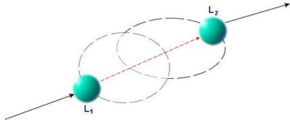
Figure 2.3 presents a scenario in which three intuitive connections are used. In this scenario, for the first intuitive connection, S = L1. Second intuitive connection connects intermediate

nodes and for the third intuitive connection T = L2.

Figure 2.3 – A scenario in which three intuitive connections are used. S – A, B – C and E – T routes are missing.

There are five types of intuitive connections.

a

(15)

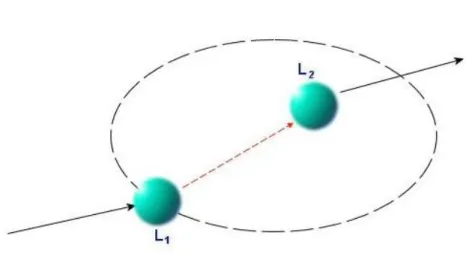
Intuitive Connection 1 – Common Parent

If there is a location P such that - L1 is a child of P

- L2 is a child of P

Figure 2.4 – Common parent intuitive connection.

The following scenario shows the usage of this type of intuitive connection.. - A route from Antalya Intercity Bus Station to Istanbul Airport is requested

- There is a basic route from Antalya Intercity Bus Station to Ankara Intercity Bus Station (L1)

- There is a basic route from Ankara Airport (L2) to Istanbul Airport

- There is no basic route between Ankara Intercity Bus Station and Ankara Airport - Ankara Intercity Bus Station and the Ankara Airport are contained in Ankara

Intuitive Connection 2 – Containment-1

Figure 2.5 – Containment-1 intuitive connection.

(16)

CHAPTER 2. INCOMPLETE INFORMATION AND VIRTUAL LINKS If there is a relationship between L1 and L2 such that

- L1 is a child of L2

The following scenario shows the usage of this type of intuitive connection..

- A route from Cayyolu (a district in Ankara) to Ulus (a district in Ankara) is requested - There is a basic route from Cayyolu to Bilkent Bus Stop (L1)

- There is a basic route from Bilkent University (L2) to Ulus

- There is no basic route from Bilkent Bus Stop to Bilkent University - Bilkent Bus Stop is contained in Bilkent University

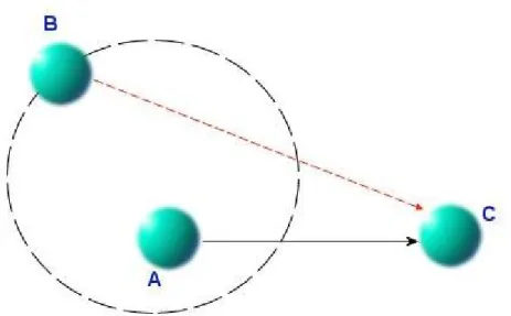
Intuitive Connection 3 – Containment-2

If there is a relationship between L1 and L2 such that

- L1 is a parent of L2

Figure 2.6 – Containment-2 intuitive connection.

- A route from Cankaya (a district in Ankara) to Bestepe (a district in Ankara) is requested

- There is a basic route from Cankaya to Kizilay (a district in Ankara – L1)

- There is a basic route from Kizilay Metro Station (L2) to Bestepe

- There is no basic route from Kizilay to Kizilay Metro Station - Kizilay Metro Station is contained in Kizilay

Intuitive Connection 4 – Neighborhood

- L1 and L2 are neighbors

(17)

Figure 2.7 – Neighborhood intuitive connection.

- A route from Cankaya (a district in Ankara) to Bestepe (a district in Ankara) is requested

- There is a basic route from Cankaya to Kizilay Main Bus Station (L1)

- There is a basic route from Kizilay Metro Station (L2) to Bestepe

- There is no basic route from Kizilay Main Bus Station to Kizilay Metro Station - Kizilay Main Bus Station and Kizilay Metro Station are neighbors

Intuitive Connection 5 – Intersection

- L1 and L2 intersects

Figure 2.8 – Intersection intuitive connection.

- A route from Kemer Town Center (a town center in Antalya) to Antalya City Center is requested

- There is a basic route from Kemer Town Center to Olympos Beach (L1) by a boat

- There is a basic route from Cirali (a town in Antaya – L2) to Antalya City Center by a

bus

- There is no basic route from Olympos Beach to Cirali - Olympos Beach and Cirali intersects

(18)

2.3 Virtual Links

In order to provide the intuitive connections, we came up with the idea of virtual links. A virtual link is a special type of link, which is maintained by the system. The users cannot maintain these links. Virtual links are maintained automatically; as users enter or delete data, the system creates or deletes virtual links accordingly. There are four types of virtual links. These types are described and illustrated in sections 2.3.1 – 2.3.4. Virtual link maintenance is described in section 2.3.5.

2.3.1 Virtual Link Type-1

If location A is in location B and a link from A to C exists, virtual link is from B to C.

Figure 2.9 – Virtual Link Type-1. A link from A to C exists in the system. B is a parent of A. Virtual link is from B to C.

This virtual link is inserted for each containment relationship. If there exists a containment relationship such that; location A resides in location B, a virtual link from A to B is added to the system.

This kind of virtual relationship “connects” the locations that are contained in the same parent location. By this, even if the system cannot find a direct route for a query, it can supply a route by using a location that is sharing a common parent.

(19)

Figure 2.10 – Virtual Link Type-2. B is a parent of A. Virtual link is from A to B.

This virtual link is inserted for each neighborhood relationship. If there is a neighborhood relationship between two locations A and B, two virtual links are added; one from A to B and the other from B to A.

Figure 2.11 – Virtual Link Type-3. A and B are neighbors.

This virtual link is inserted for each intersection relationship. If there is an intersection relationship between two locations A and B, two virtual links are added; one from A to B and the other from B to A.

(20)

Figure 2.12 – Virtual Link Type-4. A and B intersects.

2.3.5 Virtual Link Maintenance

The virtual links are all maintained by the system. Users cannot modify, delete or add virtual links to the system. We have come up with two solutions to manage virtual links and decided on the second one.

Batch Virtual Link Maintenance

In this approach, an automated script is executed and the script creates the type 1 and type 2 virtual links automatically. Before creation all the virtual links are deleted from the system. The advantage of this approach is that, there are no extra operations during data entry of the users. On the other hand, this approach leaves the database unsynchronized between script executions. The virtual links are not created immediately after data entry.

The highly coupled nature of the virtual links makes it hard to implement virtual link maintenance in real time. For the type-1 virtual links, if B is also a parent of C, the virtual link is not created. The reason for eliminating such virtual link candidates is that, with those in the system, the search algorithm gives results that are meaningless to human users.

Deletion and re-creation of around 10000 virtual links takes around 3500 ms, so running the script frequently (in the order of minutes) even if the data increases rapidly, might decrease the disadvantages due to this approach.

Real-Time Virtual Link Maintenance

This approach creates and deletes virtual links when a user-entered data is changed in the system. Virtual links are affected by containment relationships between locations and links. So, any change in these information changes the virtual links in the system. We have categorized trigger changes as follows;

- Add containment relationship (effects type-1 & type-2) - Delete containment relationship (effects type-1 & type-2) - Add link (effects type-1)

- Delete link (effects type-1)

(21)

CHAPTER 2. INCOMPLETE INFORMATION AND VIRTUAL LINKS - Add neighborhood relationship (effects type-3)

- Delete neighborhood relationship (effects type-3) - Add intersection relationship (effects type-4) - Delete intersection relationship (effects type-4)

Adding Containment Relationships

Users can enter containment relationships to the system. We are considering an atomic operation of relating a location with another, with relation type containment. Such a change in the system effects both type-1 and type-2 virtual links. The following algorithm maintains virtual links (type-1) upon entry of containment relationship.

Figure 2.13 – Pseudo code for managing type-1 virtual links upon containment addition

First part of the algorithm creates type-1 virtual links that are originating from the parent. For that, all links originating from child are retrieved.

Figure 2.14 - Pseudo code for recreating incoming type-1 virtual links

Second part, which is recreating type-1 virtual links, is a recursive algorithm. The rule of the type-1 virtual links is that, as indicated before, if destination is also a child of the parent, the link won’t be added. This is why type-1 virtual links that are ending at the new child and also children of the new child should be checked upon entry of a new containment relationship.

13

AddContainment_ManageType1(child, parent)

for each Link p originating from child

if p is not a virtual link and destination(p) is not in parent add a type 1 virtual link from parent to destination(p) end if

end for

RecreateIncomingType1Links(child)

RecreateIncomingType1Links(loc)

for each Link p ending at loc if p is a type 1 virtual link delete p

end if end for

for each Link p ending at loc if p is not a virtual link

for each parent of source(p)

if destination(p) is not in parent

add a type 1 virtual link from parent to destination(p)

end if end for end if end for

for each Location child in children(loc) RecreateIncomingType1Links(child)

(22)

Figure 2.15 - Pseudo code for managing type-2 virtual links upon containment addition

Deleting Containment Relationships

Users can delete containment relationships from the system. Such an operation effects both type-1 and type-2 virtual links in the system.

The following algorithm is for maintaining virtual links (type-1) upon deletion of a containment relationship.

Figure 2.16 – Pseudo code for managing type-1 virtual links upon containment deletion

In the first part of the algorithm, all type-1 virtual links that are created because of the relationship between the child and parent are deleted from the system. Afterwards, incoming type 1 virtual links to child are recreated.

The following algorithm maintains virtual links (type-2) upon deletion of a containment relationship.

Figure 2.17 – Pseudo code for managing type-2 virtual links upon containment deletion

Adding Links

Users can add a link from any location to any other location. Upon such a data change, type-1 virtual links should be maintained.

The following algorithm maintains virtual links (type-1) upon addition of a link.

14

DeleteContainment_ManageType2(child, parent)

for each Link p ending at parent

if p is a type 2 virtual link originating from child delete p

AddContainment_ManageType2(child, parent)

Add a virtual link from child to parent

DeleteContainment_ManageType1(child, parent)

for each Link p originating from parent

if p is a type 1 virtual link due to child parent relationship delete p

(23)

Figure 2.18 – Pseudo code for managing type-1 virtual links upon link addition

Deleting Links

Users can delete any link from the system. Upon such a data change, type 1 virtual links should be maintained.

The following algorithm maintains virtual links (type-1) upon addition of a link.

Figure 2.19 - Pseudo code for managing type-1 virtual links upon link deletion

Adding Neighborhood Relationships

Users can add neighborhood relationships between locations. Upon adding these data, the system should maintain type-3 virtual links.

Figure 2.20 – Pseudo code for managing type-3 virtual links upon neighborhood addition

Deleting Neighborhood Relationships

Users can delete neighborhood relationships between locations. Upon deleting these data, the system should maintain type-3 virtual links.

Figure 2.21 – Pseudo code for managing type-3 virtual links upon neighborhood deletion

Adding Intersection Relationships

Users can add intersection relationships between locations. Upon adding these data, the system should maintain type-4 virtual links.

15

DeleteLink_ManageType1(source, destination)

for each Link p ending at destination

if p is a type 1 virtual link that is generated due to source destination actual link

delete p end if

end for

AddNeighborhood_ManageType3(location1, location2)

add a type-3 virtual link from location1 to location2 add a type-3 virtual link from location2 to location1

DeleteNeighborhood_ManageType3(location1, location2)

delete the type-3 virtual link from location1 to location2 delete the type-3 virtual link from location2 to location1

AddLink_ManageType1(source, destination)

for each Parent parent of source

if destination is not a child of parent

add a type 1 virtual link from parent to destination end if

(24)

Figure 2.22 – Pseudo code for managing type-3 virtual links upon intersection addition

Deleting Intersection Relationships

Users can delete intersection relationships between locations. Upon deleting these data, the system should maintain type-4 virtual links.

Figure 2.23 – Pseudo code for managing type-3 virtual links upon intersection deletion

2.4 Accepted Target Set

Accepted target set is used to provide intuitive connection 3 where L2 = T and also provide

intuitive connection 1 where L2 = T. This set stores each parent of the target node, which is

not a parent of the source node. We do not add parents of both the source and the target node to the accepted target set since virtual link type-2 connects a child to its parent. Consider that they are added to the target set and consider the following scenario.

- The search is from the node S to the node T

- There exists a node, P, which is a parent of both S and T

In this scenario, S – P link (virtual link type-2) will be provided as a solution and this information is not useful for the user.

2.5 Why These Virtual Link Types

The main drawback of virtual links is that they slow down the algorithm since they introduce new edges to the graph. More edges means the algorithm will process more nodes and routes. We had two main goals while designing virtual links;

- They should cover all intuitive connections.

- Their number should be kept at minimum. The reason is to reduce the search space as much as possible. More links mean more processing.

Using these four types, it is possible to cover three intuitive connections that are described in section 2.2. These virtual links cannot cover intuitive connection 1 and intuitive connection 3 completely. The cases where L2 = T are missed since we do not have virtual links from parent

nodes to child nodes. In order to cover these cases, we have introduced the accepted target set. Instead of such an approach, we could have defined another type of virtual link, type-5; A link type that is from the parent location to the child location, i.e. the reverse of the type-2 virtual 16

DeleteIntersection_ManageType3(location1, location2)

delete the type-4 virtual link from location1 to location2 delete the type-4 virtual link from location2 to location1

AddIntersection_ManageType3(location1, location2)

add a type-4 virtual link from location1 to location2 add a type-4 virtual link from location2 to location1

(25)

link. By such a virtual link, the accepted target set would be unnecessary, but it would increase the number of virtual links. As the number of links increases, the algorithm has to process more links so the running time also increases. A comparison between the used approach and the approach with the type-5 virtual links is given in Table 2.1.

We can say that the cost increase of the approach with type-5 virtual links is more than the cost increase of the currently used approach.

Used Approach Approach With Type-3 VL

Summary Only four types of virtual links are used. Accepted target set is also used.

Five types of virtual links are used. Accepted target set is not used.

Place of Extra

Processing Whenever successor nodes of the processed node are retrieved, due to virtual links, some extra nodes are retrieved. Also, after target check, a check is done to see if the node is in the accepted target set.

Whenever successor nodes of the processed node are retrieved, due to virtual links, some extra nodes are

retrieved.

Cost of Extra

Processing Extra processing due to more successor nodes is omitted since four types of virtual links also affect the second approach the same way. Checking accepted target set is done in constant time by the help of a hash table. So, if number of processed nodes is P, the cost will change from O(P * 1) to O(P * (1 + c)) where c is a small constant.

Extra processing due to more successor nodes that are connected to the processed node by type-5 virtual links increases the processing time. If number of processed nodes without type-5 virtual links is P and if there are R number of containment relationships, the cost will change from O(P) to O(P + R).

Table 2.1 – Comparison between the applied approach and the approach with type 3 virtual links

(26)

Chapter 3 Problem Extensions

In this chapter, we explain the three extensions in our problem definition. First we explain the details of the multiple stop transportation line problem and present a solution. Then, we explain the alternative routes problem and its solution. Finally, we explain the search preferences problem and its solution.

3.1 Multiple Stop Transportation Lines

Until now, all links in the system are considered to be unrelated with each other. But in real life, links between locations can be related.

Consider a bus line in Istanbul, that is connecting four bus stops; Besiktas – Zincirlikuyu – Levent – Maslak

If the algorithm finds a route from source location to target location, in which there are two or more links from the same bus line, it should display it as just one link. So,

Source Location - … - Besiktas – Zincirlikuyu – Levent - … - Target Location is not a desired solution. Instead of this, the algorithm should provide the following route

Source Location - … - Besiktas – Levent - … - Target Location

In order to solve this problem we use a new property for the links, MultipleStopLineId. In our approach, all links, which are due to a single transportation line, will share the same MultipleStopLineId value. Other than these links, no other link will have the same value. For the above example there will be three links in the system.

- Besiktas – Zincirlikuyu - Zincirlikuyu – Levent - Levent – Maslak

We solve this problem during the display of the data to the user. During display, if we realize that two consecutive links, L1 and L2, in the solution has the same MultipleStopLineId, we display these two links as one link in which the source is the source of L1 and the target is the target of L2.

(27)

CHAPTER 3. PROBLEM EXTENSIONS

3.2 Alternative Routes

In addition to providing a route from the source location to the target location, the system should also provide alternative routes to the users.

There might be alternative routes between the selected pair in different cities or countries, using trains, using planes or using intercity buses. Inside the same city, same pair of locations might be connected by buses, ferries or metro networks.

Although “k-shortest route (path) problem” [9, 12, 16, 17, 21, 23, 24, 28] in the literature is generally studied in order to find the k optimal routes from a source to a target, it contains many similarities with the problem at hand.

In order to provide more than one route, we have to process each node more than once. We use a constant, k, in order to define the maximum number of times a node can be processed in the search algorithm. This number defines the minimum number of routes the system can provide if routes exist. It is the minimum number since there might be alternative routes that are not sharing any common node other than the source and the target nodes.

Figure 3.1 – Alternative routes example. There are four alternative routes from S to T. Three of them pass over the node B. If k = 1, two routes can be found. If k = 2, three routes can be found. If k = 3, four routes can be found.

3.3 Search Preferences

The system will allow users to enter two search preferences, which will be the input of the search algorithm.

(28)

CHAPTER 3. PROBLEM EXTENSIONS

The user should be able to exclude certain link types in his queries. For instance, a user should be able to exclude planes and intercity buses if he wants to travel by trains between cities. In order to provide this feature, we display a list of used link types to the user whenever a route is provided. User can select any number of these link types as unwanted types. After this selection user can request an alternative route. The search algorithm will this time discard a link if its type is in the excluded link types list. Discarding is a trivial issue. While processing the successors of a node in the search algorithm, types of the links that are connecting the node to its successors are checked.

In addition to excluded link types, the user should be able to select his cost preference out of two options. First option is the duration. Second option is the financial cost. So, the user should be able to specify if he is interested in a fast route that will take minimum amount of time to travel or a cheap route in which he will pay less. For each route search, user can select one option out of these two. In the search algorithm, in order to calculate the cost till the processed point, we add either durations together or the financial costs, according to the preference of the user. Since all links in the system contain information for both cost models, for any route search these two options are valid.

Throughout the thesis, whenever the cost of a link or the total cost of a route is mentioned, we are referring to one of these options. Since in both options a route or a link with a lower cost would be preferred over a higher cost route or link, it doesn’t matter which option the user has chosen.

(29)

Chapter 4 Search Algorithm

In this chapter, we first present related work for graph search algorithms, mainly about the A* graph search since our algorithm’s base is the A* search algorithm. Then we present the details of our algorithm. Afterwards we present the details of the h-value calculation together with our heuristics. After providing all the details of the algorithm, we explain the virtual link preference conditions. We conclude this chapter with an example execution scenario.

4.1 Related Work

BFS (Breadth First Search) is one of the most common graph search algorithms. Using the locations as vertices and links as edges, a graph representation is formed in memory and using BFS, a route from source to destination is searched.

BFS is an uninformed search algorithm which exhaustively searches all the nodes in the graph until it finds the desired route. It starts with the source node, and at each stage it visit one level up (source node is at level 0, successors of the source node are at level 1, etc...). On the first stage it visits all the vertices at level 1 (relative to the source node). In the second stage it visits all the vertices at level 2 and goes on like that. BFS can be considered as a “blind” search since it does not give any priority to the nodes. There are also versions of this algorithm for massive graphs [3].

DFS (Depth First Search) is very similar to BFS. Instead of processing a level after the processing of the previous level is finished, DFS processes a branch till its deepest node. There are versions [29] of this algorithm, which are handling the problems associated with duplicate nodes.

There are many algorithms [2, 5, 10] that guarantee finding the fastest path. Dijkstra’s algorithm [11] guarantees to find the fastest path (route). All nodes’ cost is initialized to a very large constant and source node’s cost is initialized as 0. At each step, the node with the least cost is processed. Whenever the target node is reached, the cost of the target node is the minimum cost between the source and the target nodes. There are algorithms [6] that guarantee to find the lowest cost route in graphs with negative weight edges. There are algorithms [1] that find the lowest cost k-link route. There are also algorithms that are running on dual graphs [30].

We do not consider these approaches as a base to our solution since they do not take advantage of additional information in the graph. They are blind search strategies and not guided. Being able to use heuristics is a mandatory requirement for us. Researches like [14] present the performance advantages of guided search strategies over blind search strategies.

(30)

CHAPTER 4. SEARCH ALGORITHM

A* search algorithm [15] is accepted as one of the most efficient route finding algorithms for graphs. The original algorithm uses a function f(n), that gives the cost of going from source location to one of the target nodes through node n. The algorithm relies on heuristics. In the pseudo code (shown in Figure 4.1), successors(p) returns the nodes that can be reached by following a single link from p. It is assumed that the queue maintains an ordering by f-value automatically.

f(n) = g(n) + h(n)

g(n) is the cost of the route so far (cost between the source node and n) and h(n) is the estimated cost from n to the target node. In this h function, heuristics comes into play and used for estimating the remaining cost. According to the value of f(n) a route is given higher or lower priority.

With this algorithm, one can use several heuristics for prioritizing routes. The advantage is that different heuristics can be added to the algorithm as new optimization ways are discovered since the heuristic implementations are separated from the algorithm core.

Figure 4.1 – Pseudo code of the A* search algorithm

IDA* [18] is a modified version of the A* algorithm. In this version, iterative-deepening approach [25] is applied to the A* algorithm. This algorithm suffers from the usage of only a limited amount of memory. So, it suffers from excessive node regeneration.

RBFS [19] is a recursive algorithm that attempts to mimic the operation of standard best-first search using only linear space. Its structure is similar to recursive depth-first search. Instead of continuing indefinitely down the current path, it keeps track of the f value of the best alternative route available from any ancestor of the current node. If the current node exceeds f-value limit, the recursion unwinds back to the alternative path. As the recursion unwinds, RBFS replaces the f-value of each node align the path with the best f-value of its children. By this, the algorithm remembers the f-value of the best leaf in the forgotten subtree. Similar to IDA*, RBFS also suffers from excessive node generation.

22

A*(start,goal)

var closed <- the empty set var q <- make_queue(start) while q is not empty

var p <- remove_first(q) var x <- the last node of p if x in closed continue end if if x = goal return p end if add x to closed

for each y in successors(x) enqueue(q, p, y)

end for

end while

(31)

MA* [8] is the memory bounded version of A* algorithm. In contrast to IDA*, its memory limit is not fixed; the algorithm can take advantage of the whole available memory.

SMA* [26, 27] has some improvements over MA*. It proceeds just like A*. When the memory is full, it discards the node with the worst value from the queue and backups the f-value of the forgotten node to its parent. By this, the ancestor of a forgotten subtree knows the quality of the best route in that subtree. When all the nodes in the queue have f-values greater than the forgotten node’s f-value, the node is regenerated.

SMAG* is a graph search extension of SMA*. This algorithm prunes a node whenever a lower cost route from source to that node is found. By this way, its entire subtree is removed from the search space and the node can be explored again.

A new algorithm which is similar to SMAG* is introduced in [31]. The difference of this approach is to propagate the change instead of pruning when a lower cost route is found to a previously explored node. The change is propagated to the node’s descendants. In [14], a new approach which is using A* in combination with a technique based on landmarks and the triangle inequality is presented.

**4.2 A*CD Algorithm Details**

There are many approaches and algorithms for finding routes in graphs. Among these alternatives we have selected the A* search algorithm as the base. As explained in the previous section, A* algorithm’s structure allows heuristics to be integrated to the search algorithm.

A* search guarantees to find the fastest route if the heuristic function is monotone [15, 31]. A heuristic function h is monotone if for each node n and successor node n'_,

h(n) ≤ h(n') + c(n, n')

where c(n, n') is the cost of the link from n to n'_{. Our heuristic function does not meet this} criteria so A*CD does not guarantee to find the fastest route.

A*CD starts from the source node and at each step successors of the current node are retrieved from the database. Upon successor retrieval, heuristics are applied to the successor nodes, some of them are eliminated and the others are added to the priority queue to be further processed.

In the original A* algorithm heuristics are applied to estimate the cost to the target node. Assume that we are processing a node that is corresponding to location L. Original A* algorithm takes successors of L, and for each node S in successors(L) it applies the heuristics and calculates an estimate; cost of the route with the lowest cost, which is passing through S

f(n) = g(n) + h(n)

where g(n) is the actual cost of the route so far and h(n) is the estimated cost to reach from the current node to the target node. In the original A* algorithm, f value is calculated for all nodes 23

(32)

S in successors(L) and the successor is added to the queue together with its f value. As the f value of a route decreases, it is more favorable since it means its cost estimate is lower. Lower cost means better route.

In our approach, calculation of g-value is done according to the costs of the links used so far. Assume that the algorithm is processing location L. This location has been retrieved from the queue in order to be processed. For each location that is in the queue, the cost to reach from the source location to that node is also stored. So, while processing successors of L, adding the link cost to the cost of L is enough to calculate g-value.

Figure 4.2 – An example scenario for g-value calculation.

For Figure 4.2, values near links indicate their cost. c values are the costs (financial) of the links and d values are the durations of the links. Assume that search is started from node S. L is the currently processed node; it has been retrieved from the queue. There are three successor nodes of L; S1, S2 and S3. For each successor, a g-value must be calculated. If the user has selected duration as his point of interest, g-values will be as follows;

- g(S1) = d1 + d2 + d3 - g(S2) = d1 + d2 + d4 - g(S3) = d1 + d2 + d5

If the user has selected financial cost as his point of interest, g-values will be calculated as follows;

- g(S1) = c1 + c2 + c3 - g(S2) = c1 + c2 + c4 - g(S3) = c1 + c2 + c5

(33)

Calculation of h-value is done in three steps. In the first step the distance between the currently processed node and the target node is calculated by using the geographic coordinates of the nodes.

This value is then normalized in order to match its unit (kilometers) with the unit of the g-value (duration or financial cost, depends on the choice of the user).

This value is then increased or decreased by the heuristics [4, 7, 13, 20, 22]. According to the data existing in the system, the algorithm modifies the value of the estimated cost.

All heuristics are combined together to modify the estimated cost value. We do not have any constraint for the number of heuristics that are applied. They might be considered as rules [4] which are affecting the estimated cost.

An important advantage of this approach is its flexibility. As the system operates, there will be new ideas for collecting new information about locations and links. New heuristics, which are relying on the new data, can easily be integrated to this system.

While one heuristic increases the estimated cost, another one might decrease it. It is like saying, “This route uses very few numbers of hops and is cheap, but it takes too long”. By using this approach, we believe we are reflecting the advantages and disadvantages of routes to the algorithm in a suitable way.

Figure 4.3 – Multiple routes reaching to the same node.

Another important thing to be noted on the algorithm is its support for supplying alternative routes. As indicated previously in Chapter 3, we want the algorithm to provide several alternative routes to the user. In the classical A* search algorithm structure, no such support exists. Whenever a node in successors set of the currently processed node is seen, the algorithm checks to see if the node has been previously added to the queue. If so, the successor node is skipped. Consider the graph in Figure 4.3. In this graph, there are two 25

(34)

alternative routes from S to T. Consider that Bus link is processed before Dolmuş link. In this case, Dolmuş link won’t be processed by the algorithm, since the algorithm has already reached L1 and L1 has already been added to the queue (containing S as its ancestor and Bus link as its ancestor connecting link).

In order to modify this approach to support finding k-shortest routes, we are storing more than one instance of the same node in the queue. For the above example, two instances of node L1 will be stored in the queue with our approach. One instance contains Dolmuş as the ancestor connecting link and the other instance contains Bus as the ancestor connecting link.

The queue (defined at line 6) is used to store the nodes that should be processed. The nodes in this queue are ordered according to their f-value. For initialization, start node is added to the queue. Queue might contain more than one instance of the same node if more than one route has been found to that node.

The set “visitedNodes” is used to store nodes that have been reached in the search. This set might be considered as a permanent backup location for nodes. As indicated, the queue stores only nodes to be processed. So, if a node is processed it is removed from the queue. On the other hand, we need removed nodes’ information (in order to track the route from the target to the source by visiting ancestor node of each node). This set is used to provide this information.

“excludedLinkTypes” is a set, in which elements are link types. This set is added to the algorithm in order to give the user a chance to exclude one or more link types from the search. Line 22 is related with accepted target set. The “incompleteResults” set in the algorithm stores the found routes that are from source node to a node in the accepted target set. If no route between source and target is found, these results are displayed to the user.

In the original A* algorithm goal check is done inside the body of the for loop that is starting at line 26. Instead of this approach, we are doing this check inside the body of the while loop that is starting at line 8. By this, when the target node is reached, it is again processed and added to the priority queue. But this time its favorability is multiplied with a high constant (by heuristic 7). By this, if a node has more than one link to the goal target, an order between those two links can also be done by our system.

Also checks like the one at Line 2 of the “enqueue” method can be done by this approach. Consider the case in we have locations S, P and T with the following conditions

- S is the source node - T is the target node

- There is a user entered link from S to T

- There is a type 2 virtual link from S to P (because of containment relationship)

- There is a type 1 virtual link from P to T (because of containment relationship and S – T link)

In these conditions, if original A* approach is used, as the algorithm is processing node S, it will find P – T link, and since it reaches us to the target, it will return the result immediately, which is an incorrect behavior. But when we process this link by our regular procedures, it is being eliminated because of the check at line 2 of the enqueue method.

(35)

Figure 4.4 – Pseudo code of A*CD algorithm

Whenever a node is retrieved from the queue, a check is done to see if the node has been processed before (line 10). In this check, value of k is important. If the node has been visited k times, it is considered to be processed before so it is skipped (pseudo code for that function is provided in Figure 4.7).

If the node turns out to be the target node, the route from source node to the target node is added to the found routes set (line 15). If the node turns out to be in the accepted target set, it is added to the incomplete results set (line 23). There is an important difference between these two cases. If the node is the target, the algorithm does not continue with the successors of the node. On the other hand, if the node is in the accepted target set, it is added to the incomplete results but in addition to that, successors of the node are also processed.

27

1 A*CD(source, target, excludedLinkTypes) 2 var visitedNodes <- empty set

3 var acceptedTargets <- getAcceptedTargets(source, target) 4 var routes <- empty set

5 var incompleteResults <- empty set 6 var q <- make_queue(source)

7 var k <- number of routes to be found 8 while q is not empty

9 var node <- remove_first(q) 10 if (processedBefore(node)) 11 continue

12 end if

13 addToVisitedSet(node) 14 if node == goal

15 addToFoundRoutes(routes, visitedNodes, node) 16 if (routes.Count == k) 17 return routes 18 else 19 continue 20 end if 21 end if

22 if node in acceptedTargets and L.getType() != virtual link 23 addToIncompleteResults(incompleteResults, visitedNodes, node) 24 end if

25 var routeFromSource <- createRouteFromSource(node) 26 for each Link L originating from node

27 if L.getType() in excludedLinkTypes 28 continue

29 end if

30 if L.getType() is virtual link and L.actualLink().getType() 31 in excludedLinkTypes 32 continue 33 end if 34 if L.getDestination() in routeFromSource.NodeSet 35 continue 36 end if 37 enqueue(node, L, routeFromSource) 38 end for 39 end while

40 add incompleteResults to routes set 41 return routes

(36)

After the target checks, successors of the node are retrieved from the database. For each successor, excluded link type check is done. If the successor passes this check, the route till now (the route starting from the start node and ending at the currently processed node) is checked; if the route contains the successor, successor is skipped. After passing these checks, enqueue method is called.

Figure 4.5 – Pseudo code of enqueue method

Figure 4.6 – Indirect virtual link loop. If node B is being processed, B-C-A route might occur if this check is not done. The virtual link from B to C is created because of the B contains A relationship and A to C link. So, in the graph it is not a loop but when the actual links in real life are considered, this condition is a loop.

28

1 enqueue(node, link)

2 if checkType2Type1VirtualLinkChain() is true 3 return

4 end if

5 var newNode <- link.getTarget() 6 newNode.ancestor <- node

7 newNode.ancestorConnectingLink <- link 8 var favorability <- applyAllHeuristics() 9 if (favorability < threshold) 10 return 11 end if 12 if (checkIndirectVirtualLinkLoop()) 13 return 14 end if

15 var gVal <- node.distanceTillNow + link.cost

16 var fVal <- gVal + calculateHValue(node, newNode, link, favorability) 17 addToQueue(newNode, fVal)

(37)

Figure 4.7 – Pseudo codes of the helper methods

Enqueue method first checks for virtual link chains (line 2). Figure 4.6 shows an example virtual link chain. Then, the new node is created (line 5). This new node is the one that will be added to the queue (if it passes the checks). Its ancestor is initialized as the currently processed node and its ancestor connecting link is initialized as the currently processed link. Than, at line 15, a favorability value is calculated. This is done by applying all heuristics one by one. If the favorability value turns out to be lower than the favorability threshold, ft, new node is not added to the queue.

Finally, the f-value is calculated by adding g-value with h-value.

4.3 Calculation of h-value and Heuristics

h(n) is the estimated cost of reaching from node n to target. We are calculating this value in three parts. First, we are calculating the geographical distance between node n and the target. After this, we are normalizing this value since the distance is in miles but we need a cost measure for summing h-value with g-value. Finally, we are applying several heuristic functions in order to calculate a favorability value r(n). According to the data entered by the users, this favorability value is increased or decreased. After this favorability value calculation is done, it’s inverse (1 / r(n)) is multiplied by the normalized estimated cost in order to give the final h(n) value.

29

1 processedBefore(node)

2 var tmpNodeArray <- visitedNodes.getNodeArray(node.Id) 3 if tmpNodeArray = null 4 return false 5 end if 6 if tmpNodeArray.Count < k 7 return false 8 end if 9 return true 1 addToVisitedSet(node)

2 var tmpNodeArray <- visitedNodes.getNodeArray(node.Id) 3 if tmpNodeArray = null 4 tmpNodeArray <- createEmptyArray() 5 end if 6 tmpNodeArray.addElement(node) 7 visitedNodes.addNodeArray(tmpNodeArray) 1 createRouteFromSource(node)

2 var route <- emptyRoute 3 var currentNode <- node

4 var link <- null 5 route.addNode(node)

6 while currentNode != start node

7 link <- currentNode.getAncestorConnectingLink() 8 currentNode <- currentNode.getAncestor()

9 route.addNode(currentNode) 10 route.addLink(link)

(38)

Calculating Geographical Distance

Figure 4.8 – Distance calculation

Normalization of the Distance

The cost estimate is based on the geographical distance between the new node and the target node. But this value, alone, is not enough for a proper estimate. The unit of this estimate is kilometers; it is the distance between the new node and the target node. On the other hand, unit of the cost till now is either a currency (financial cost) or time. So addition of these values with different units won’t give us a proper overall f-value.

In order to normalize the value, we have developed two approaches. After developing and testing the first approach, we have realized that it has some disadvantages. Because of this, we have developed another approach.

Normalization – Approach 1

In this approach, we are normalizing the estimated cost by using three other values; - Distance between the new node and the target

- Distance between the source and the new node - Actual cost from the source node to the new node

Figure 4.9 – Normalizing the distance. c1 is the actual cost between the source node and the currently processed node. There might be more than one link, only total cost of the route is important. c2 is the actual cost of the link connecting node and new node. Normalized estimated cost value is calculated according to c1, c2 and distance between new node and the target node.

30

var x <- 69.1 * (Lattitudet – Lattitudes)

var y <- 69.1 * (Longitudet - Longitudes) * Cosine(Lattitudet / 57.3)

(39)

The aim of this approach is to exploit the existing information to estimate a cost. We know the distance between the source node and the new node. We also know the cost between these nodes. Also, we know the distance between the new node and the target node. So, by a simple ratio calculation we can have a cost estimate between the new node and the target node.

distance(source, newNode) / (c1 + c2) = distance(newNode, source) / x

Although this approach seems as an applicable one, it has two main disadvantages. First of all, since type-2 virtual links (the links from the child nodes to the parent nodes) have a cost of 0, for nodes that are reachable by these links, the cost is underestimated.

Another disadvantage is the variable nature of the links. Consider that the query is between two very distant nodes (like two locations in different countries). Also consider that the route till now (route from the source node to the new node) contains only close locations to the source node. In this case, the estimate will be very different from the actual cost since links between close locations have different cost characteristics than links between distant locations. To be more specific, consider that the user has selected duration as the cost model. For close locations, x kilometers might take 2x minutes. On the other hand, for distant locations, if a plane will be used, 800x kilometers take x minutes.

Normalization – Approach 2

This approach provides a hard-coded conversion between miles and cost. The pseudo-code is given in Figure 4.10.

Figure 4.10 - Pseudo code of the applied normalization approach

The threshold values (t values) and multiplier values (m values) are different for duration and financial cost choices.

These are the hard-coded estimates. In a way, we are transferring our route expertise to the system by this normalization method. For example, if the distance is below 100 miles, we can say that the duration estimate will be distance * 1. Meaning each mile will take 1 minute to travel.

Of course, this approach has also disadvantages. Consider two distance values, d1 = t1 – 1 and

d2 = t1 + 1. Although they have a very small difference, their cost estimate will be very

different. 31 Normalize(distance) if distance < t1 return distance * m1 else if distance < t2 return distance * m2 else if distance < t3 return distance * m3 else return distance * m4 end if