NOISE ENHANCED DETECTION
a thesis
submitted to the department of electrical and
electronics engineering
and the institute of engineering and sciences
of bilkent university
in partial fulfillment of the requirements
for the degree of
master of science
By
Suat Bayram
I certify that I have read this thesis and that in my opinion it is fully adequate, in scope and in quality, as a thesis for the degree of Master of Science.
Asst. Prof. Dr. Sinan Gezici (Supervisor)
I certify that I have read this thesis and that in my opinion it is fully adequate, in scope and in quality, as a thesis for the degree of Master of Science.
Prof. Dr. Orhan Arıkan
I certify that I have read this thesis and that in my opinion it is fully adequate, in scope and in quality, as a thesis for the degree of Master of Science.
Asst. Prof. Dr. ˙Ibrahim K¨orpeo˘glu
Approved for the Institute of Engineering and Sciences:
Prof. Dr. Mehmet Baray
ABSTRACT
NOISE ENHANCED DETECTION
Suat Bayram
M.S. in Electrical and Electronics Engineering
Supervisor: Asst. Prof. Dr. Sinan Gezici
June 2009
Performance of some suboptimal detectors can be improved by adding indepen-dent noise to their measurements. Improving the performance of a detector by adding a stochastic signal to the measurement can be considered in the frame-work of stochastic resonance (SR), which can be regarded as the observation of “noise benefits” related to signal transmission in nonlinear systems. Such noise benefits can be in various forms, such as a decrease in probability of error, or an increase in probability of detection under a false-alarm rate constraint. The main focus of this thesis is to investigate noise benefits in the Bayesian, mini-max and Neyman-Pearson frameworks, and characterize optimal additional noise components, and quantify their effects.
In the first part of the thesis, a Bayesian framework is considered, and the previous results on optimal additional noise components for simple binary hypothesis-testing problems are extended to M-ary composite hypothesis-testing problems. In addition, a practical detection problem is considered in the Bayesian framework. Namely, binary hypothesis-testing via a sign detector is studied for antipodal signals under symmetric Gaussian mixture noise, and the effects of shifting the measurements (observations) used by the sign detector are investi-gated. First, a sufficient condition is obtained to specify when the sign detector
based on the modified measurements (called the “modified” sign detector) can have smaller probability of error than the original sign detector. Also, two suf-ficient conditions under which the original sign detector cannot be improved by measurement modification are derived in terms of desired signal and Gaussian mixture noise parameters. Then, for equal variances of the Gaussian components in the mixture noise, it is shown that the probability of error for the modified detector is a monotone increasing function of the variance parameter, which is not always true for the original detector. In addition, the maximum improve-ment, specified as the ratio between the probabilities of error for the original and the modified detectors, is specified as 2 for infinitesimally small variances of the Gaussian components in the mixture noise. Finally, numerical examples are presented to support the theoretical results, and some extensions to the case of asymmetric Gaussian mixture noise are explained.
In the second part of the thesis, the effects of adding independent noise to measurements are studied for M-ary hypothesis-testing problems according to the minimax criterion. It is shown that the optimal additional noise can be represented by a randomization of at most M signal values. In addition, a convex relaxation approach is proposed to obtain an accurate approximation to the noise probability distribution in polynomial time. Furthermore, sufficient conditions are presented to determine when additional noise can or cannot improve the performance of a given detector. Finally, a numerical example is presented.
Finally, the effects of additional independent noise are investigated in the Neyman-Pearson framework, and various sufficient conditions on the improv-ability and the non-improvimprov-ability of a suboptimal detector are derived. First, a sufficient condition under which the performance of a suboptimal detector can-not be enhanced by additional independent noise is obtained according to the Neyman-Pearson criterion. Then, sufficient conditions are obtained to specify
when the detector performance can be improved. In addition to a generic con-dition, various explicit sufficient conditions are proposed for easy evaluation of improvability. Finally, a numerical example is presented and the practicality of the proposed conditions is discussed.
Keywords: Hypothesis testing, noise enhanced detection, Bayes decision rule,
¨
OZET
G ¨
UR ¨
ULT ¨
U ˙ILE GEL˙IS¸T˙IR˙ILM˙IS¸ SEZ˙IM
Suat Bayram
Elektrik ve Elektronik M¨uhendisli˘gi B¨ol¨um¨u Y¨uksek Lisans
Tez Y¨oneticisi: Asst. Prof. Dr. Sinan Gezici
Haziran 2009
Optimal olmayan bazı detekt¨orlerin girdisine ba˘gımsız g¨ur¨ult¨u eklenerek, de-tekt¨or¨un performansı artırılabilir. Bu olay, do˘grusal olmayan sistemlerde sinyal iletimi sırasında g¨ur¨ult¨u yararının g¨ozlemlenmesi ¸seklinde de tanımlanabilen stokastik rezonans (SR) kavramı ile ilintilidir. G¨ur¨ult¨u yararı, hata ihtimalinin azalması ya da belirli yanlı¸s tespit seviyesi altında do˘gru tespit ihtimalinin art-ması gibi bir¸cok farklı ¸sekilde g¨ozlemlenebilir. Bu tezin temel olarak yo˘gunla¸stı˘gı konu, g¨ur¨ult¨u yararının Bayesian, minimax ve Neyman-Pearson kriterlerinde ¸calı¸sılması ve optimal g¨ur¨ult¨un¨un formunun ve etkilerinin incelenmesidir.
Tezin ilk kısmında, ikili basit hipotez testleri i¸cin optimal g¨ur¨ult¨u formu ile ilgili literat¨urdeki ¨onceki sonu¸clar, ¸coklu bile¸sik hipotez testlerine geni¸sletilmektedir. Buna ek olarak, iki kutuplu sinyallerin Gauss karı¸sımı
(Gaus-sian mixture) g¨ur¨ult¨us¨u altında i¸saret detekt¨or¨u ile tespit edilmesi problemi,
Bayesian kriterine g¨ore analiz edilmektedir. Bu analizde, i¸saret detekt¨or¨u tarafından kullanılan g¨ozlemleri kaydırmanın sonu¸cları ara¸stırılmaktadır. ˙Ilk olarak, kaydırılmı¸s g¨ozlemler kullanan i¸saret detekt¨or¨un¨un, orijinal i¸saret de-tekt¨or¨unden daha d¨u¸s¨uk hata olasılı˘gına sahip olması i¸cin bir yeterli ko¸sul sunul-maktadır. Bunun yanında, orijinal detekt¨or¨un geli¸stirilemedi˘gi iki yeterli ko¸sul elde edilmektedir. Bu yeterli ko¸sullar, sinyal ve Gauss karı¸sımı g¨ur¨ult¨us¨un¨un
parametreleri cinsinden bulunmaktadır. Gauss karı¸sımı g¨ur¨ult¨us¨undeki Gauss bile¸senlerinin standard sapmaları e¸sit oldu˘gu zaman, hata ihtimali de˘gistirilmi¸s detekt¨or i¸cin monoton artan bir fonksiyondur. Bu durum, orijinal detekt¨or i¸cin her zaman ge¸cerli de˘gildir. Buna ek olarak, Gauss karı¸sımı g¨ur¨ult¨us¨undeki Gauss bile¸senlerin standard sapmaları sıfıra gitti˘gi zaman, orijinal hata ihtimalinin de˘gistirilmi¸s detekt¨or¨un hata ihtimaline oranının, yani geli¸sim oranının, en fazla ikiye e¸sit oldu˘gu g¨osterilmektedir. Son olarak, sayısal ¨orneklerle teorik sonu¸clar desteklenmekte ve teorik sonu¸cların simetrik olmayan Gauss karı¸sımı g¨ur¨ult¨us¨une nasıl geni¸sletilebilece˘giyle ilgili yorumlar yapılmaktadır.
Tezin ikinci kısmında, ¸coklu (M’li) hipotez testlerinde, detekt¨orlerin kul-landı˘gı g¨ozlemlere ba˘gımsız g¨ur¨ult¨u eklemenin, minimax kriteri altındaki etk-ileri analiz edilmektedir. Optimal g¨ur¨ult¨un¨un ihtimal yo˘gunluk fonksiy-onunun en fazla M farklı de˘ger icin sıfırdan farklı olabilece˘gi ispatlanmak-tadır. Buna ek olarak, polinom zamanda optimal g¨ur¨ult¨un¨un ihtimal yo˘gunluk fonksiyonunun yakla¸sık olarak “convex relaxation” y¨ontemiyle elde edilebilece˘gi g¨osterilmektedir. Ayrıca, detekt¨or performansının g¨ur¨ult¨uyle hangi durum-larda geli¸stirilip geli¸stirilemiyece˘giyle ilgili yeterli ko¸sullar sunulmaktadır. Son b¨ol¨umde ise, sayısal bir ¨ornek ¨uzerine ¸calı¸sılmaktadır.
Son olarak, Neyman-Pearson kriteri altında, g¨ozleme ba˘gımsız g¨ur¨ult¨u ekle-menin detekt¨or performansı ¨uzerindeki etkileri incelenmektedir. Bu ba˘glamda, optimal olmayan bir detekt¨or¨un performansının geli¸stirilip geli¸stirilemiyece˘gi du-rumlarla ilgili yeterli ko¸sullar ¸cıkarılmaktadır. ˙Ilk olarak, Neyman-Pearson kriter-ine g¨ore, optimal olmayan bir detekt¨or¨un performansının hangi durumda g¨ozleme ba˘gımsız g¨ur¨ult¨u ekleme yoluyla geli¸stirilemiyece˘giyle ilgili yeterli ko¸sul sunul-maktadır. Daha sonra, detekt¨or¨un geli¸stirilebilmesiyle ilgili yeterli ko¸sullar elde edilmektedir. Genel ko¸sulların yanında, geli¸stirilebilirlili˘gin kolay test edilebilme-sine imkan sa˘glayan ¸ce¸sitli yeterli ko¸sullar da ¨onerilmektedir. Son olarak, sayısal ¨ornekler sunulmakta ve ¨onerilen ko¸sulların pratik de˘gerleri tartı¸sılmaktadır.
Anahtar Kelimeler: Hipotez testi, g¨ur¨ult¨uyle geli¸stirilmi¸s sezim, Bayes kuralı, minimax, Neyman-Pearson, stokastik rezonans (SR), i¸saret detekt¨or¨u.
ACKNOWLEDGMENTS
I was so lucky to have Asst. Prof. Dr. Sinan Gezici as my advisor. He has been one of the few people who had vital influence on my life. His endless energy, perfectionist personality and inspirational nature have been a great admiration for me. It was a real privilege and honor for me to work with such a visionary and inspirational advisor. I would like to, especially, thank him for providing me great research opportunities and environment.
I also extend my special thanks to Sara Bergene, Zakir S¨ozduyar, Mehmet Barı¸s Tabakcıo˘glu, Mustafa ¨Urel, Abd¨ulkadir Eryıldırım, Saba ¨Oz, Mahmut Yavuzer, Hamza So˘gancı, M. Emin Tutay, Yasir Karı¸san, Sevin¸c Figen ¨Oktem, Aslı ¨Unl¨ugedik, and Ba¸sak Demirba˘g for being wonderful friends and sharing unforgettable moments together. Also I would like to thank Professor Orhan Arıkan and Asst. Prof. Dr. ˙Ibrahim K¨orpeo˘glu for agreeing to serve on my thesis committee. I would also like to thank T ¨UB˙ITAK for its financial support which was vital for me.
I would also like to thank Elif Eda Demir, who has been a true friend for my life, for the spectacular moments we had.
Finally, I would like to give a special thank to my mother Zehra, and my brothers Yakup, Cavit and Acar Alp for their unconditional love and support throughout my studies. They mean everything to me. I have much gratitude towards my mother for helping me believe that there is nothing one cannot accomplish.
Contents
1 Introduction 1
1.1 Objectives and Contributions of the Thesis . . . 1
1.2 Organization of the Thesis . . . 5
2 Noise Enhanced Detection in the Bayesian Framework and Its Application to Sign Detection under Gaussian Mixture Noise 7 2.1 Noise Enhanced M-ary Composite Hypothesis-Testing in the Bayesian Framework . . . 8
2.1.1 Generic Solution . . . 8
2.1.2 Special Cases . . . 11
2.1.3 A Detection Example . . . 14
2.2 Noise Enhanced Sign Detection under Gaussian Mixture Noise . . 17
2.2.1 Signal Model . . . 17
2.2.2 Formulation of Optimal Measurement Shifts . . . 19
2.2.3 Conditions for Improvability and Non-improvability of De-tection . . . 20
2.2.4 Performance Analysis of Noise Enhanced Detection . . . . 23
2.2.5 Numerical Results . . . 32
2.3 Concluding Remarks and Extensions . . . 37
3 Noise Enhanced M-ary Hypothesis-Testing in the Minimax Framework 40 3.1 Problem Formulation . . . 41
3.2 Noise Enhanced Hypothesis-Testing . . . 42
3.3 Numerical Results . . . 46
3.4 Concluding Remarks . . . 48
4 On the Improvability and Non-improvability of Detection in the Neyman-Pearson Framework 50 4.1 Signal Model . . . 51 4.2 Non-improvability Conditions . . . 52 4.3 Improvability Conditions . . . 54 4.4 Numerical Results . . . 59 4.5 Concluding Remarks . . . 63
List of Figures
2.1 Additional independent noise c is added to observation x in order to improve the performance of the detector φ(·). . . . 9 2.2 Bayes risk versus α for A = 2 and σ = 1. . . 16 2.3 Bayes risk versus c for A = 2 and σ = 1. . . 16 2.4 Mean values (xj’s) in a symmetric Gaussian mixture noise for
M = 8, and signal amplitude A. . . 27
2.5 Mean values (xj’s) in a symmetric Gaussian mixture noise for
M = 8, signal amplitude A, and additional noise c. . . 28
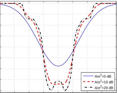
2.6 (a) In the conventional case, the mean values (xj’s) of the Gaus-sian mixture noise that are in the interval [−A, A] determine the probability of error. (b) When a constant noise term c is added, the mean values (xj’s) of the Gaussian mixture noise that are in the interval [−A − c, A − c] determine the probability of error. . . 29 2.7 Probability of error versus A/σ2 for symmetric Gaussian
mix-ture noise with M = 10, where the center values are
±[0.02 0.18 0.30 0.55 1.35] with corresponding weights of
2.8 Probability of error in (2.47) versus c for various A/σ2 values for
the scenario in Fig. 2.7. . . 33 2.9 The improvability function in (2.48) and the optimal additional
signal value copt in (2.46) versus A/σ2 for the scenario in Fig. 2.7. 34
2.10 Probability of error versus A for symmetric Gaussian mixture noise with σi = 0.1 for i = 1, . . . , M and M = 10, where the center values are ±[0.02 0.18 0.30 0.55 1.35] with corresponding weights of [0.167 0.075 0.048 0.068 0.142]. . . 34 2.11 The improvability function in (2.48) and the optimal additional
signal value copt in (2.46) versus A for the scenario in Fig. 2.10. . 35
2.12 Probability of error versus σ for A = 1 and for symmetric Gaus-sian mixture noise with M = 12, where the center values are
±[0.0965 0.2252 0.4919 0.6372 0.8401 1.0151] with corresponding
weights of [0.1020 0.0022 0.2486 0.0076 0.1293 0.0103]. . . 36 2.13 The optimal additional noise coptin (2.46) versus σ for the scenario
in Fig. 2.12. . . 37 2.14 The improvability function in (2.48) versus σ for the scenario in
Fig. 2.12. . . 38
3.1 Maximum of the conditional risks versus η for the original and the noise-modified detectors for A = 1, B = 2.5, σ = 0.1, w1 = 0.5
and w2 = 0.5. . . 46
3.2 Probability mass function of optimal additional noise for various threshold values when the parameters are taken as A = 1, B = 2.5,
3.3 Original and noise-modified maximum of the conditional risks vs
σ graph for the parameters taken as η = 1.8, A = 1, B = 2.5, w1 = 0.5 and w2 = 0.5. . . 49
4.1 The improvability function obtained from Proposition 3 for various values of A, where ρ1 = 0.1, ρ2 = 0.2, µ1 = 2, and µ2 = 3. . . 61
4.2 Detection probabilities of the original and noise modified detectors versus σ for A = 2, ρ1 = 0.1, ρ2 = 0.2, µ1 = 2, and µ2 = 3. . . 61
4.3 The improvability function obtained from Proposition 3 for various values of A in the case of sign detector where ρ1 = 0.1, ρ2 = 0.2,
Chapter 1
Introduction
1.1
Objectives and Contributions of the Thesis
Performance of some suboptimal detectors can be improved by adding indepen-dent noise to their measurements. Improving the performance of a detector by adding a stochastic signal to the measurement is referred to as noise enhanced detection [1], [2]. Noise enhanced detection can also be considered in the frame-work of stochastic resonance (SR), which can be regarded as the observation of “noise benefits” related to signal transmission in nonlinear systems [3]-[17]. Such noise benefits can be in various forms, such as an increase in output signal-to-noise ratio (SNR) [5], [3], a decrease in probability of error [18], or an increase in probability of detection under a false-alarm rate constraint [1], [17].
Although adding noise to a system commonly degrades its output, SR presents an exception to that intuition, which is observed under special circum-stances. The SR was first studied in [3] to explain the periodic recurrence of ice gases. In that work, presence of noise was taken into account to explain a natural phenomenon. Since then, the SR concept has been employed in numerous non-linear systems, such as optical, electronic, magnetic, and neuronal systems [8].
The first experimental verification of the SR phenomenon was the investigation of the behavior of the Schmitt trigger in an electronic bistable system [19].
Considering the probability of error as the performance criterion, it is shown in [18] that the optimal additional signal that minimizes the probability of er-ror of a suboptimal detector has a constant value. In other words, addition of a stochastic signal to the measurement corresponds to a shift of the measure-ments in that scenario. Hence, when the aim is to minimize the probability of error, improvement of detector performance by utilizing SR can be regarded as threshold adaptation, which has been applied in various fields, such as in radar problems [20]. Although the formulation of the optimal signal value is provided in [18], no studies have investigated sufficient conditions for improvability and non-improvability of specific suboptimal detectors according to the minimum probability of error criterion, and quantified performance improvements that can be achieved by measurement modifications. In addition, the effects of additional noise have not been investigated for composite hypothesis-testing problems in the Bayesian framework.
An important application of the results in [18] includes the investigation of the effects of additional noise (effectively, measurement shifts) on sign detec-tors that operate under Gaussian mixture noise. Motivated by the fact that, under zero-mean Gaussian noise, signals with opposite polarities minimize the error probability of a sign detector based on correlation outputs [21], antipodal signaling with sign detection has been extensively used in communications sys-tems [22]. In fact, sign detectors can be employed as suboptimal detectors in symmetric non-Gaussian noise environments as well due to their low complex-ity [23]. Therefore, it is of interest to investigate techniques that preserve the low complexity structure of the sign detector but improve the overall receiver performance by modifying the measurements (observations) used by the detec-tor. In this thesis, the effects of adding a stochastic signal to measurements are
investigated for sign detection of antipodal signals under symmetric Gaussian mixture noise. The Gaussian mixture model is encountered in many practi-cal scenarios, such as characterization of multiple-access-interference (MAI) [24], ultra-wideband (UWB) communications systems [25], localization [26] and ac-quisition [27] problems.
In Chapter 2 of the thesis, optimal additional noise is shown to have a con-stant value for M-ary composite hypothesis-testing problems in the Bayesian framework, which extends the results in [18]. In other words, the optimal ad-ditional noise corresponds to a shift of the measurements for M-ary composite hypothesis-testing problems as well. Then, the effects of measurement shifts are investigated for sign detection of antipodal signals under symmetric Gaussian mixture noise according to the minimum probability of error criterion. First, a sufficient condition is obtained for measurement shifts to reduce the probability error of a sign detector in terms of desired signal and Gaussian mixture noise parameters. Then, two conditions under which the performance of the original detector cannot be improved are derived. Also, for equal variances of the Gaus-sian components in the mixture noise, the probability of error for the modified detector is characterized as a monotone increasing function of the variance. It is also shown via numerical examples that the original detector does not have this property in general. In addition, a theoretical performance comparison is made between the original and the modified detectors for small variances of the Gaussian components in the mixture noise, and it is shown that the maximum ratio between the probabilities of error for the original and the modified detectors is equal to two. As a byproduct of this result, sufficient conditions for improv-ability and non-improvimprov-ability of the sign detector are obtained for infinitesimally small variance values. Finally, numerical examples are presented to support the theoretical results, and some concluding remarks are made.
In addition to the Bayesian criterion, performance of some detectors can be evaluated according to the minimax criterion in the absence of prior information about the hypotheses [21], [28]. The study in [29] utilizes the results in [18] and [1] in order to investigate optimal additional noise for suboptimal variable detectors in the Bayesian and minimax frameworks. Although the formulation of optimal additional noise is studied for a binary hypothesis-testing problem in [29], no studies have investigated M-ary hypothesis problems under the minimax framework, and provided the structure of the optimal noise probability density functions (PDFs) and sufficient conditions for the improvability and the non-improvability of a given detector.
In Chapter 3 of this thesis, noise enhanced detection is studied for M-ary hypothesis-testing problems in the minimax framework. First, the formulation of optimal additional noise is provided for an M-ary hypothesis-testing problem according to the minimax criterion. Then, it is shown that the optimal additional noise can be represented by a randomization of no more than M signal levels. In addition, a convex relaxation approach is proposed to obtain an accurate ap-proximation to the noise PDF in polynomial time. Also, sufficient conditions are provided regarding the improvability and non-improvability of a given detector via additional noise.
In the absence of prior information about the hypotheses, the Neyman-Pearson criterion considers the maximization of detection probability under a constraint on the probability of false alarm [21]. In the framework of noise enhanced detection, the aim is to obtain the optimal additional noise that max-imizes the probability of detection under a constraint on the probability of false alarm [1], [17]. In [1], a theoretical framework is developed for this problem, and the PDF of optimal additional noise is specified. Specifically, it is proven that optimal noise can be characterized by a randomization of at most two discrete
signals, which is an important result as it greatly simplifies the calculation of op-timal noise PDFs. Moreover, [1] provides sufficient conditions under which the performance of a suboptimal detector can or cannot be improved via additional independent noise. The study in [17] focuses on the same problem and obtains the optimal additional noise PDF via an optimization theoretic approach. In addition, it derives alternative improvability conditions for the case of scalar observations.
In Chapter 4 of this thesis, new improvability and non-improvability con-ditions are proposed for detectors in the Neyman-Pearson framework, and the improvability conditions in [17] are extended. The results also provide alternative sufficient conditions to those in [1]. In other words, new sufficient conditions are derived, under which the detection probability of a suboptimal detector can or cannot be improved by additional independent noise, under a constraint on the probability of false alarm. All the proposed conditions are defined in terms of the probabilities of detection and false alarm for specific additional noise values without the need for any other auxiliary functions employed in [1]. In addition to deriving generic conditions, simpler but less generic improvability conditions are provided for practical purposes. The results are compared to those in [1], and the advantages and disadvantages are specified for both approaches. In other words, comments are provided regarding specific detection problems, for which one approach can be more suitable than the other. Moreover, the improvabil-ity conditions in [17] for scalar observations are extended to both more generic conditions and to the case of vector observations.
1.2
Organization of the Thesis
The organization of the thesis is as follows. In Chapter 2, optimal additional noise is characterized for M-ary composite hypothesis-testing problems in the Bayesian
framework, and the effects of additional noise are investigated for conventional sign detectors under symmetric Gaussian mixture noise.
In Chapter 3, noise benefits are investigated for M-ary hypothesis-testing problems under the minimax framework. Both the optimal additional noise characterization is provided, and a technique for obtaining the optimal addi-tional noise components is proposed.
In Chapter 4, new improvability and non-improvability conditions are pro-posed for suboptimal detectors in the Neyman-Pearson framework, and the im-provability conditions in [17] are extended. The results also provide alternative sufficient conditions to those in [1].
Chapter 2
Noise Enhanced Detection in the
Bayesian Framework and Its
Application to Sign Detection
under Gaussian Mixture Noise
This chapter is organized as follows. In Section 2.1, optimal additional noise is characterized for M-ary composite hypothesis-testing problems according to the Bayesian criterion. Then, based on the results in Section 2.1, noise enhanced detection is studied for sign detectors under Gaussian mixture noise in the re-maining sections. In Section 2.2.1, the system model is introduced, and the Gaussian mixture measurement noise is described. Then, Section 2.2.2 studies the optimal additional independent noise for minimizing the probability of deci-sion error for a sign detector under symmetric Gaussian mixture noise. In Section 2.2.3, conditions on desired signal amplitude and/or the parameters of Gaussian mixture noise are derived in order to specify whether the performance of the detector can be improved. After that, the probability of error performance of the noise enhanced detector is investigated, and a monotonicity property of the
probability of error and the maximum improvement ratio are derived in Section 2.2.4. Finally, numerical examples are studied in Section 2.2.5, and concluding remarks and extensions are presented in Section 2.3.
2.1
Noise Enhanced M-ary Composite
Hypothesis-Testing in the Bayesian Framework
2.1.1
Generic Solution
Consider the following M-ary composite hypothesis-testing problem:
Hi : pXθ (x) , θ ∈ Λi , i = 0, 1, . . . , M − 1 , (2.1) where Hi denotes the ith hypothesis and pXθ (x) represents the probability den-sity function (PDF) of observation X for a given value of Θ = θ. Each ob-servation (measurement) x is a vector with K components; i.e., x ∈ RK, and Λ0, Λ1, . . . , ΛM −1 form a partition of the parameter space Λ. The prior distribu-tion of the unknown parameter Θ, denoted by w(θ), is assumed to be known, considering a Bayesian framework.
A generic decision rule can be defined as
φ(x) = i , if x ∈ Γi , (2.2)
for i = 0, 1, . . . , M −1, where Γ0, Γ1, . . . , ΓM −1form a partition of the observation space Γ.
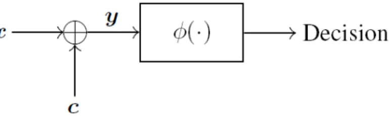
As shown in Fig. 2.1, the aim is to add noise to the original observation x in order to improve the performance of the detector according to the Bayesian criterion. By adding noise c to the original observation x, the modified obser-vation is formed as y = x + c, where c has a PDF denoted by pC(·), and is
Figure 2.1: Additional independent noise c is added to observation x in order to improve the performance of the detector φ(·).
independent of x. It is assumed that the detector φ , described by (2.2), is fixed, and the only means for improving the performance of the detector is to optimize the additional noise c. In other words, the aim is to find pC(·) that minimizes the Bayes risk r(φ); that is,
poptC (c) = arg min pC(c)
r(φ) , (2.3)
where the Bayes risk is given by [21]
r(φ) = E{RΘ(φ)} =
Z
Λ
Rθ(φ)w(θ) dθ , (2.4)
with Rθ(φ) denoting the conditional risk that is defined as the average cost of decision rule φ for a given θ ∈ Λ. The conditional risk can be calculated from [21] Rθ(φ) = E{C[φ(Y ), Θ] | Θ = θ} = Z Γ C[φ(y), θ] pY θ(y) dy , (2.5) where pY
θ(y) is the PDF of the modified observation for a given value of Θ = θ, and C[i, θ] is the cost of selecting Hi when Θ = θ, for θ ∈ Λ. Thus, r(φ) can be expressed as r(φ) = Z Λ Z Γ C[φ(y), θ] pY θ(y) w(θ) dy dθ. (2.6)
Due to the addition of independent noise, the modified observation has the following PDF:
pYθ(y) = Z
RK
Then, from (2.6) and (2.7), the following expressions are obtained: r(φ) = Z Λ Z Γ Z RK C[φ(y), θ] pX θ (y − c) pC(c) w(θ) dc dy dθ (2.8) = Z RK pC(c) ·Z Λ Z Γ C[φ(y), θ]pX θ (y − c) w(θ) dy dθ ¸ dc (2.9) = Z RK pC(c) f (c) dc (2.10) = E{f (C)} (2.11) where f (c)=. Z Λ Z Γ C[φ(y), θ] pX θ (y − c) w(θ) dy dθ . (2.12)
From (2.11), it is observed that the solution of (2.3) can be obtained by assigning all the probability to the minimizer of f (c); i.e.,
poptC (c) = δ(c − c0) , (2.13)
where
c0 = arg min
c f (c). (2.14)
In other words, the optimal additional noise that minimizes the Bayes risk can be expressed as a constant corresponding to the minimum value of f (c). Of course, when f (c) has multiple minima, then the optimal noise PDF can be represented as pC(c) = PNi=1λiδ(c − c0i), for any λi ≥ 0 such that
PN
i=1λi = 1, where
c01, . . . , c0N represent the values corresponding to the minimum values of f (c).
The main implication of the result in (2.13) is that among all PDFs for the additional independent noise c, the ones that assign all the probability to a single noise value can be used as the optimal additional signal components in Fig. 2.1. In other words, in the Bayesian framework, addition of independent noise to observations corresponds to shifting the decision region of the detector.
2.1.2
Special Cases
The analysis in the previous section considers a Bayes risk based on a very generic cost function C[j, θ], which can assign different costs even to the same decision j for a given true hypothesis θ ∈ Λi when different values of θ in set Λi are considered. In this section, various special cases are studied for some specific structures of the cost function. In addition, the binary hypothesis-testing problem (M = 2) is analyzed in more detail.
If it is assumed, for all i, j, that the cost of deciding Hj when Hi is true is the same for all θ ∈ Λi (i.e., if a uniform cost is assumed in each Λi for
i = 0, 1, . . . , M − 1), the cost function satisfies
C[φ(y) = j , θ] = Cji , ∀θ ∈ Λi , ∀i, j ∈ {0, 1, . . . , M − 1} , (2.15) where Cji is a non-negative constant that is independent of θ [21]. Then, f (c) in (2.12) becomes f (c) = Z Λ Z Γ C[φ(y), θ] pX θ (y − c) w(θ) dy dθ = M −1X i=0 Z Λi à M −1X j=0 Z Γj Cji pXθ (y − c) dy ! w(θ) dθ = M −1X i=0 M −1X j=0 Cji Z Γj Z Λi pX θ (y − c)w(θ) dθ dy = M −1X i=0 M −1X j=0 Cjifji(c) (2.16) where fji(c)=. Z Γj Z Λi pXθ (y − c)w(θ) dθ dy . (2.17)
In addition to (2.15), if uniform cost assignment (UCA) is considered, the costs are specified as Cji = 1 for j 6= i and Cji = 0 for j = i. In other words, the correct decisions are assigned zero cost, whereas the wrong ones are assigned
unit cost. In this case, f (c) in (2.16) becomes f (c) = M −1X i=0 M −1X j=0 j6=i fji(c) = 1 − M −1X i=0 fii(c) . (2.18)
Next, let M = 2 (i.e., binary hypothesis-testing) and assume uniform costs in Λi for i = 0, 1. Then, f (c) can be calculated as follows:
f (c) = 1 X i=0 1 X j=0 Cjifji(c) = 1 X i=0 1 X j=0 Cji Z Γj Z Λi pX θ (y − c)w(θ) dθ dy = C10 Z Γ1 Z Λ0 pX θ (y − c)w(θ) dθ dy + C00 Z Γ0 Z Λ0 pX θ (y − c)w(θ) dθ dy + C01 Z Γ0 Z Λ1 pXθ (y − c)w(θ) dθ dy + C11 Z Γ1 Z Λ1 pXθ (y − c)w(θ) dθ dy = π1C01+ π0C00+ Z Γ1 " (C10− C00) Z Λ0 pX θ (y − c)w(θ) dθ − (C01− C11) Z Λ1 pXθ (y − c)w(θ) dθ # dy , (2.19)
where the following relation is employed in obtaining the final expression: Z Γ0 Z Λi pX θ (y − c)w(θ) dθ dy = πi− Z Γ1 Z Λi pX θ (y − c)w(θ) dθ dy , (2.20) for i = 0, 1, with πi = P (Hi) = R Λiw(θ) dθ .
Then, the Bayes risk in (2.10) can be expressed from (2.19) as
r(φ) = Z RK pC(c) f (c) dc = E{f (C)} = π1C01+ π0C00− E{g(C)} , (2.21) where g(c) = Z Γ1 " − (C10− C00) Z Λ0 pX θ (y − c)w(θ) dθ + (C01− C11) Z Λ1 pX θ (y − c)w(θ) dθ # dy . (2.22)
From (2.21), it is observed that r(φ) is minimized for pC(c) = δ(c − c0),
where
c0 = arg max
Therefore, the optimal additional noise that minimizes the Bayes risk can be expressed as a constant corresponding to the maximum value of g(c).
In order to obtain a more explicit expression for g(c), the following result is employed [21]. pX(y − c|Θ ∈ Λ i) = 1 πi Z Λi pX θ (y − c)w(θ) dθ , i = 0, 1. (2.24) Then, g(c) in (2.22) can be expressed as
g(c) = Z RK φ(y) " (C01− C11) Z Λ1 pX θ (y − c)w(θ) dθ − (C10− C00) Z Λ0 pX θ (y − c)w(θ) dθ # dy (2.25) = Z RK φ(x + c) h (C01− C11)π1pX(x|θ ∈ Λ1) − (C10− C00)π0pX(x|θ ∈ Λ0) i dx , (2.26)
where the result in (2.24), as well as a change of variables (x = y − c) are used in obtaining the final result. If we define a new function h(x) as
h(x) = (C01− C11)π1pX(x|θ ∈ Λ1) − (C10− C00)π0pX(x|θ ∈ Λ0) , (2.27) we then have g(c) = Z RK φ(x + c)h(x) dx . (2.28)
As can be seen from (2.28), g(c) is the correlation between the decision function and h(x).
If we also assume that correct decisions have zero cost, and wrong ones have unit cost, we have r(φ) = π1− E{g(C)} and
h(x) = π1pX(x|θ ∈ Λ1) − π0pX(x|θ ∈ Λ0) . (2.29)
For simple hypotheses (i.e., when Λ0 and Λ1 contain single elements), (2.29)
yields h(x) = π1pX1 (x) − π0pX0 (x), which is the result obtained in [18]. In Section
2.2, the result for simple hypotheses is used to investigate noise enhanced sign detectors under Gaussian mixture noise.
2.1.3
A Detection Example
In this section, the following composite hypothesis-testing problem is studied in order to present an example of the theoretical results obtained in the previous sections.
H0 : θ ∈ Λ0 = [−α, 0] ,
H1 : θ ∈ Λ1 = (0, 2α] , (2.30)
where α is a known positive real number. For a given value of Θ = θ, the observation X has the following PDF:
pXθ (x) = 1 3 £ γ(x; θ − A, σ2) + γ(x; θ, σ2) + γ(x; θ + A, σ2)¤ , (2.31) where γ(x; µ, σ2) =. √1 2πσexp ³ −(x−µ)2σ22 ´
. In other words, the observation is dis-tributed as the mixture of three Gaussian distributions with the same variance
σ2 and means θ − A, θ, and θ + A. In addition, the prior distribution of Θ is
modeled by a uniform random variable between −α and 2α, which is denoted as Θ ∼ U[−α , 2α]. Therefore, the prior probabilities of the hypotheses can be obtained as π0 = P (H0) =
R0
−α3α1 dθ = 1/3 and π1 = P (H1) =
R2α
0 3α1 dθ = 2/3 .
The sign detector is considered as the decision rule in this example, which is expressed as φ(y) = 1 if y ≥ 0 0 if y < 0 . (2.32)
The aim is to obtain the optimal value of additional signal c such that y = x + c results in the minimum Bayes risk for this composite hypothesis-testing problem (cf. (2.3)).
Assuming uniform costs in Λ0 and Λ1 and for UCA, the optimal value of c
can be obtained from (2.14), (2.17) and (2.18), or from (2.23), (2.28) and (2.29). When the solution based on (2.14), (2.17) and (2.18) is considered, f (c) can be
obtained as f (c) = 1 − f00(c) − f11(c). From (2.17), f00(c) and f11(c) can be
expressed for Θ ∼ U[−α , 2α] as
f00(c) = 1 3α Z 0 −α Z 0 −∞ pXθ (y − c) dy dθ , (2.33) f11(c) = 1 3α Z 2α 0 Z ∞ 0 pX θ (y − c) dy dθ . (2.34)
Then, after some manipulation, f (c) = 1 − f00(c) − f11(c) can be obtained, from
(2.31), (2.33) and (2.34), as f (c) = 1 − f00(c) − f11(c) = 2 3− 1 9α µZ 2α 0 vθ(c) dθ − Z 0 −α vθ(c) dθ ¶ , (2.35) where vθ(c)= Q. µ −θ + A − c σ ¶ + Q µ −θ − c σ ¶ + Q µ −θ − A − c σ ¶ . (2.36)
Therefore, the optimal value of c can be calculated from (2.14) and (2.35) as
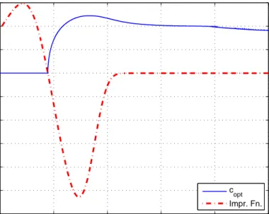
c0 = arg max c ½Z 2α 0 vθ(c) dθ − Z 0 −α vθ(c) dθ ¾ . (2.37)
In Fig. 2.2, the Bayes risks are plotted against α for the original sign detector (i.e., without additional signal c) and for the noise enhanced sign detector (i.e., with optimal additional signal c0) when A = 2 and σ = 1. Note from (2.11) that
the Bayes risks are given by r(φ) = f (0) and r(φ) = f (c0) for the original and
the noise enhanced sign detectors, respectively. It is observed from the figure that there is significant improvement for small values of α and the amount of improvement decreases as α increases. For example, for α = 0.5, the Bayes risks are 0.429 and 0.323, respectively, for the conventional and the noise enhanced sign detectors, whereas they are 0.298 and 0.262 for α = 1.5 .
In Fig. 2.3, the Bayes risk is plotted versus additional signal c when A = 2 and σ = 1 for various values α . For each α, there is a unique minimizer of the Bayes risk for a positive value of c. In addition, it is observed that the optimal additional signal value c0 in (2.37) decreases as α increases. In fact, for large
0 1 2 3 4 5 0.1 0.15 0.2 0.25 0.3 0.35 0.4 0.45 0.5 α Bayes Risk Original Noise Enhanced
Figure 2.2: Bayes risk versus α for A = 2 and σ = 1.
−10 −5 0 5 10 0.2 0.3 0.4 0.5 0.6 0.7 c Bayes Risk α=1 α=2 α=3
values of α, c0 goes to zero, which implies that the detector cannot be improved
by additional noise; that is, the original detector is non-improvable, which is in compliance with the result in Fig. 2.2.
2.2
Noise Enhanced Sign Detection under
Gaussian Mixture Noise
After showing, in the previous section, that an optimal additional noise corre-sponds to a shift of the measurements used by the detector, this section inves-tigates the effects of measurement shifts for sign detection of antipodal signals under symmetric Gaussian mixture noise.
2.2.1
Signal Model
Consider the following measurement (observation) model
x = A b + n , (2.38)
where b ∈ {−1, +1} represents the equiprobable binary symbol to be detected,
A > 0 is the known amplitude coefficient,1 and n is the measurement noise,
which is modeled as symmetric Gaussian mixture noise. The PDF of the noise is given by pN(x) = M X i=1 wiψi(x − xi) , (2.39) where wi ≥ 0 for i = 1, . . . , M , PM i=1wi = 1, and ψi(x) = 1 √ 2π σi exp µ −x2 2 σ2 i ¶ , (2.40)
1The results in the thesis can be extended to A < 0 cases as well, by switching the decision regions of the detector in (2.42).
for i = 1, . . . , M . Due to the symmetry assumption, xi = −xM −i+1, wi = wM −i+1 and σi = σM −i+1 for i = 1, . . . , bM/2c.
The symmetric Gaussian mixture model specified above is observed in many practical scenarios [25]-[30]. One important scenario is multiuser wireless com-munications, in which the desired signal is corrupted by interference from other users as well as zero-mean Gaussian background noise. In that case, the over-all noise has a symmetric Gaussian mixture model when the user symbols are symmetric and equiprobable (e.g., ±1 with equal probability) [23].
The problem can be stated as the following binary hypothesis test
H0 : X ∼ pN(x + A) ,
H1 : X ∼ pN(x − A) , (2.41)
where hypotheses H0 and H1 correspond to b = −1 and b = +1 cases,
respec-tively. The following conventional sign detector is considered to determine the index of the true hypothesis, which is expressed as
φ(x) = 0 , x < 0 1 , x > 0 . (2.42)
In the case of x = 0, the detector decides H0 or H1 randomly (i.e., with equal
probabilities). It is well-known that the conventional detector in (2.42) is not optimal in general for Gaussian mixture noise [18], [31]. However, its main advantage is that it has very low complexity, which makes it very practical for low cost applications. Therefore, the main aim in this work is to keep the low complexity of the detector but to modify the measurement in (2.38) in order to improve detection performance.
2.2.2
Formulation of Optimal Measurement Shifts
Instead of the original measurement x, consider a noise modified version of the measurement as
y = x + c , (2.43)
where c represents additional independent noise term.
As studied in [18] and in Section 2.1, the optimal additional noise c that minimizes the probability of decision error2 is a constant that solves the following
maximization problem:
copt = arg max
c Z ∞
−∞
φ(y + c) [pN(y − A) − pN(y + A)] dy , (2.44) where pN(·) represents the PDF of the measurement noise in (2.38).
For the detector in (2.42), the optimal additional noise in (2.44) is given by
copt = arg max
c Z ∞
−c
[pN(y − A) − pN(y + A)] dy , (2.45) which, after some manipulation, can be expressed, from (2.39), as
copt = arg max
c M X i=1 wi · Q µ −c − A − xi σi ¶ − Q µ −c + A − xi σi ¶¸ , (2.46) where Q(x) = √1 2π R∞ x e−t 2/2
dt represents the Q-function. Note that the
opti-mization in (2.46) can be performed over c ≥ 0 only, since it can be shown that the term in the square brackets is an even function of c for the symmetric Gaussian mixture noise model.
The probability of decision error when a constant noise c is added in (2.43) is given by [18] P(c) = 1 2− 1 2 M X i=1 wi · Q µ −c − A − xi σi ¶ − Q µ −c + A − xi σi ¶¸ . (2.47)
2This criterion is equivalent to the minimization of the Bayes risk for uniform cost assign-ment and equal priors [21].
When the optimal value of c is calculated as in (2.46), PSR = P(copt) specifies
the error probability obtained via measurement modification. The conventional case corresponds to using no additional noise, i.e., Pconv = P(0). Note that
copt = 0 corresponds to the non-improvability case, in which it is not possible to
improve the detector performance by adding noise to the measurement; that is, PSR = Pconv. On the other hand, if PSR < Pconv, the detector is improvable [1].
One justification for using additional noise (measurement shifts) to improve performance of suboptimal detectors as in (2.42) instead of employing an optimal detector based on the likelihood ratio test is reduced implementation complexity [1]. Instead of calculating the likelihood ratio for each observation, the detector in (2.42) just checks the sign of the observation shifted by copt. Note that the
calculation of copt requires the solution of the optimization problem in (2.46),
but that problem needs to be solved only when the noise statistics and/or the signal amplitude change.
2.2.3
Conditions for Improvability and Non-improvability
of Detection
In this section, sufficient conditions are derived in order to determine whether additional noise can enhance the performance of the conventional detector in (2.42) in the presence of symmetric Gaussian mixture measurement noise. Such improvability and non-improvability conditions carry practical importance, since determination of whether additional noise is useful or not based on desired signal and measurement noise parameters helps specify when to solve the optimization problem in (2.46) for the optimal additional noise.
First, a sufficient condition on the signal amplitude and the measurement noise statistics is obtained in order for additional noise to improve detection performance.
Proposition 1: The detector in (2.42) is improvable if the signal amplitude
A in (2.38) and the measurement noise specified by (2.39) and (2.40) satisfy
M X i=1 wi σ3 i (A + xi) e −(A+xi)2σ2 2 i < 0 . (2.48)
Proof: From (2.46), a first-order necessary condition for optimal additional noise value can be obtained by equating the first derivative with respect to c to zero. M X i=1 wi √ 2π σi à e−(−c−A−xi) 2 2σ2i − e− (−c+A−xi)2 2σ2i ! = 0 . (2.49)
Note that the condition in (2.49) is satisfied by the conventional solution, i.e., for c = 0. In addition, the second derivative at c = 0 can be calculated from (2.49) as M X i=1 wi √ 2π σ3 i à −(A + xi) e −(A+xi)2σ2 2 i − (A − xi) e −(A−xi)2σ2 2 i ! . (2.50)
Due to the symmetry of the Gaussian mixture PDF, the expression in (2.50) is always positive when the condition in the proposition is satisfied. Since the first derivative is zero and the second derivative is positive at c = 0, it is a minimum point of the objective function in (2.46). Therefore, (2.47) implies that there exists c 6= 0 such that PSR(c) < Pconv, which proves the improvability of the
detector. ¤
Proposition 1 provides a simple sufficient condition to determine if the use of additional noise can improve the performance of the detector in (2.42). When the condition in (2.48) is satisfied, the optimal additional noise can be calculated from (2.46) (which is non-zero since the system is improvable), and the updated measurement in (2.43) can be used for improved error performance.
Similar to determining the improvability of the system, it is also important to know when the system cannot be improved via additional noise. Such a knowl-edge prevents efforts for solving (2.46) to find the additional noise, which yields
copt = 0 when the system is non-improvable. In the following, two conditions are
provided to classify the system as non-improvable.
Proposition 2: Assume that the variances of the Gaussian components in
the mixture noise, specified by (2.39) and (2.40), converge to infinity; that is, σ2
i → ∞ for i = 1, . . . , M. Then, the detector in (2.42) is non-improvable. Proof: This result can be proven by showing that lim
σ2
1,...,σ2M→∞
P (c)
P (0) = 1, where
P (c) is as in (2.47). In other words, no improvement can be obtained for any
value of c. Hence, the detector is non-improvable. ¤
The main implication of Proposition 2 is that when the variance of each Gaussian component in the Gaussian mixture noise is very large, the conventional decision rule, which decides H0 for negative measurements and H1 otherwise, has
lower probability of error than any other decision rule that applies the sign rule in (2.42) on shifted measurements as in (2.43) for c 6= 0. In other words, for large variances, copt = 0 and PSR = Pconv.
Another non-improvability condition can be obtained when the signal ampli-tude A in (2.38) is larger than or equal to all the mass points in the Gaussian mixture noise.
Proposition 3: Assume that the signal amplitude A in (2.38) is larger than
or equal to the maximum of the mean values of the Gaussian components in the Gaussian mixture in (2.39); that is,
A ≥ max
i=1,...,M{xi} . (2.51)
Then, the detector in (2.42) is non-improvable.
Proof: The first-order necessary optimality condition in (2.49) is given by M X i=1 wi σi e−(c+A+xi) 2 2σ2i = M X i=1 wi σi e−(c−A+xi) 2 2σ2i . (2.52)
Due to the symmetry of the Gaussian mixture noise, (2.52) can be expressed as bM/2cX i=1 wi σi à e−(c+A+xi) 2 2σ2i + e− (c+A−xi)2 2σ2i ! = bM/2cX i=1 wi σi à e−(−c+A+xi) 2 2σ2i + e− (−c+A−xi)2 2σ2i ! . (2.53) Since A ≥ max
i=1,...,M{xi}, A+xi ≥ 0 and −A+xi ≤ 0 for i = 1, . . . , M. Then, for
c > 0, it is observed that e− (c+A+xi)2 2σ2i < e− (−c+A+xi)2 2σ2i and e− (c+A−xi)2 2σ2i < e− (−c+A−xi)2 2σ2i
for i = 1, . . . , M . Therefore, the term on the right-hand-side (RHS) of (2.53) is always larger than that on the left-hand-side (LHS) for c > 0. Similarly, it can be shown that the term on the LHS of (2.53) is always larger than that on the RHS for c < 0. The equality is satisfied only when c = 0. In addition, the second derivative at c = 0, given in (2.50), is always negative since A ± xi ≥ 0 for i = 1, . . . , M. Hence, c = 0 is the unique maximum of the problem in (2.46). ¤
Proposition 3 states that if the signal amplitude A is larger than or equal to all the mean values of the Gaussian components in the mixture noise, then there is no need to search for optimal additional noise as copt = 0 in that case, which implies
that the conventional algorithm cannot be improved. In fact, if A > max i=1,...,M{xi} and if σi’s in (2.40) are very small, then the conventional system can have very small probability of error, hence, may not need performance improvement in some cases.
2.2.4
Performance Analysis of Noise Enhanced Detection
After the investigation of improvability and non-improvability conditions in the previous section, this section focuses on some properties of noise enhanced detec-tion, and theoretical limits on performance improvements that can be obtained by adding noise to measurements.
First, the effects of additional noise are investigated as a function of the standard deviations of the Gaussian noise components in the Gaussian mixture noise specified by (2.39) and (2.40). Let σ = [σ1· · · σM] represent the standard deviation terms in (2.40). Then, the probability of decision error of the noise enhanced detector can be expressed, from (2.46) and (2.47), as
PSR(σ) = 1 2 − 1 2maxc M X i=1 wi · Q µ −c − A − xi σi ¶ − Q µ −c + A − xi σi ¶¸ . (2.54) In the conventional case, no additional noise is used; hence, the probability of decision error is given by
Pconv(σ) = 1 2− 1 2 M X i=1 wi · Q µ −A − xi σi ¶ − Q µ A − xi σi ¶¸ . (2.55)
For certain parameters of the Gaussian mixture noise, the probabilities of decision error in (2.54) and (2.55) may not be monotonically decreasing as the standard deviations, σ1, . . . , σM, decrease. Although this might seem counter-intuitive at first, it mainly due to the multi-modal nature of the Gaussian mixture distri-bution. In Section 2.2.5, numerical examples are provided to illustrate that be-havior. Although the probabilities of error can exhibit non-monotonic behaviors in general, the following proposition states that for equal standard deviations, a decrease in the standard deviation value can never result in an increase in the probability of decision error for the noise enhanced detector.
Proposition 4: Assume σi = σ for i = 1, . . . , M . Then, PSR(σ) in (2.54) is
a monotone increasing function of σ.
Proof: When σi = σ for i = 1, . . . , M , PSR(σ) in (2.54) is expressed as
PSR(σ) = 1 2− 1 2 M X i=1 wi · Q µ −copt(σ) − A − xi σ ¶ − Q µ −copt(σ) + A − xi σ ¶¸ , (2.56)
where copt(σ) represents the maximizer of the summation term in (2.54), which
satisfies the following first and second derivative conditions3
M X i=1 wi σ µ e−(−copt(σ)−A−xi) 2 2σ2 − e− (−copt(σ)+A−xi)2 2σ2 ¶ = 0 , (2.57) M X i=1 wi σ3 h (−copt(σ) − A − xi) e− (−copt(σ)−A−xi)2 2σ2 − (−copt(σ) + A − xi) e− (−copt(σ)+A−xi)2 2σ2 i < 0 . (2.58)
In order to prove the monotonicity of PSR(σ) in (2.56) with respect to σ, the
first derivative of PSR(σ) is calculated as follows:
dPSR(σ) dσ = 1 2 M X i=1 wi √ 2π σ2 ( · −dcopt(σ) dσ σ + copt(σ) + A + xi ¸ e−(copt(σ)+A+xi) 2 2σ2 − · −dcopt(σ) dσ σ + copt(σ) − A + xi ¸ e−(copt(σ)−A+xi) 2 2σ2 ) , (2.59) which can be manipulated to obtain
dPSR(σ) dσ = − 1 2√2π dcopt(σ) dσ M X i=1 wi σ · e−(copt(σ)+A+xi) 2 2σ2 − e− (copt(σ)−A+xi)2 2σ2 ¸ + 1 2√2π σ2 M X i=1 wi " (copt(σ) + A + xi) e− (copt(σ)+A+xi)2 2σ2 − (copt(σ) − A + xi) e− (copt(σ)−A+xi)2 2σ2 # . (2.60)
Since copt(σ) satisfies (2.57), the first term in (2.60) becomes zero. In
addi-tion, (2.58) implies that the second term in (2.60) is always positive. Therefore,
dPSR(σ)/dσ > 0 is satisfied; hence, PSR(σ) is a monotone increasing function of
σ. ¤
It is noted from the proof of Proposition 4 that the result is valid also for asymmetric Gaussian mixture noise. In other words, as long as σi = σ for
i = 1, . . . , M , PSR(σ) in (2.54) is a monotone increasing function of σ.
3The inequalities in (2.57) and (2.58) can be obtained similar to those in (2.49) and (2.50) by taking the derivatives of the summation term in (2.54), which is equal to that in (2.46), with respect to c.
One implication of Proposition 4 is that for equal σ1, . . . , σM in (2.40), the noise enhanced detector utilizes any decrease in the standard deviations for de-creasing the probability of decision error. In other words, a decrease in the stan-dard deviation can never increase error probability. This statement is not true in general for the conventional algorithm, which does not employ any additional noise. Addition of noise provides such a desirable monotonicity property since it effectively provides an adaptive detector structure depending on the characteris-tics of the noise. Note that addition of a constant to the decision variable, as in (2.43), for the detector in (2.42) is equivalent to using the original observation but adjusting the threshold of the detector.
The condition in Proposition 4 about equal σ1, . . . , σM values may not hold in all scenarios. However, one important scenario in which such Gaussian mixture noise components are observed includes measurement noise that is composed of zero-mean Gaussian noise and discrete noise components. An important ex-ample of such a scenario is binary detection in the presence of multiple-access interference (MAI) [23], where the measurement is modeled as
x = A1b1+
K X
k=2
Akbk+ n , (2.61)
with bi ∈ {±1} and n representing a zero-mean Gaussian noise component. The aim is to detect b1 in the presence of MAI,
PK
k=2Akbk, and background noise, n. Therefore, the total noise,PKk=2Akbk+ n, can be modeled as Gaussian mixture noise with mean values at PKk=2Akbk for all possible b2, . . . , bK values (that is, for [b2, . . . , bK] ∈ {±1}K−1) and standard deviation terms being all equal to that of the background noise term n. Therefore, the result in Proposition 4 applies in this practical scenario.
As studied in Proposition 2, additional noise cannot improve detector perfor-mance for very large variances of the Gaussian mixture noise. Another important case is to investigate the behavior of the noise enhanced detector for very small variances. As σi → 0 for i = 1, . . . , M , the probability of decision error in (2.55)
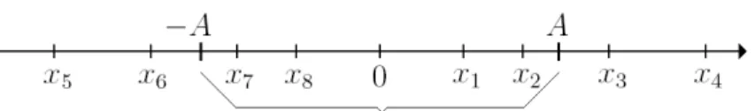
Figure 2.4: Mean values (xj’s) in a symmetric Gaussian mixture noise for M = 8, and signal amplitude A.
for the conventional algorithm can be expressed as4
Pconv = 1 2 − 1 2 M X i=1 wiu(A − |xi|) , (2.62)
where u(·) is the unit step function defined as
u(x)=. 1 , x > 0 0.5 , x = 0 0 , x < 0 . (2.63)
Similarly, as σi → 0 for i = 1, . . . , M , the probability of decision error in (2.54)
for the noise enhanced algorithm is given by PSR = 1 2 − 1 2maxc M X i=1 wiu(A − |xi+ c|) . (2.64)
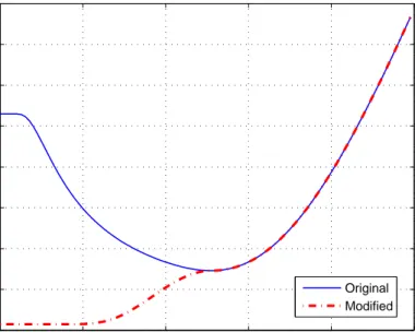
The expressions in (2.62) and (2.64) provide a simple interpretation of the probability of decision error. For example, consider the values of x1, . . . , xM and
A as in Fig. 2.4. Since the probability of error expression in (2.62) states that
the xivalues that are between −A and A contribute to the summation term, only the weights w1, w2, w7 and w8 are employed in the calculation of the probability
of error for the settings in Fig. 2.4. For the noise enhanced scenario, various values of c in (2.64) correspond to various shifts of the interval in Fig. 2.4 as shown in Fig. 2.5. Then, the value of c that results in the minimum probability of error is selected as the additional noise component.
4x
Figure 2.5: Mean values (xj’s) in a symmetric Gaussian mixture noise for M = 8, signal amplitude A, and additional noise c.
The previous interpretation of noise enhanced detection for very small vari-ance values facilitates calculation of theoretical limits on performvari-ance improve-ments that can be obtained via additional noise.
Proposition 5: Let M be an even number5 and 0 < x
1 < · · · < xM/2 without
loss of generality. As σi → 0 for i = 1, . . . , M , the maximum improvement of the
sign detector in (2.42) under symmetric Gaussian mixture noise given by (2.39) and (2.40) is specified as max A,x1,...,xM,w1,...,wM Pconv PSR = 2 , (2.65)
which is achieved when there exists i ∈ {1, . . . , M/2 − 1} such that xi+1 > A > (xi+ xM/2)/2 .
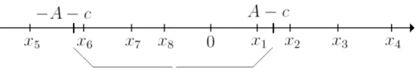
Proof: Let xi < A < xi+1 for any i ∈ {1, . . . , M/2 − 1}. Note that there is no need to consider i = M/2 since there can be no improvement by adding noise to the measurement for A > xM/2 = max{xi}, as stated in Proposition 3. From (2.62), the probability of error for the conventional case can be calculated for xi < A < xi+1 as (c.f. Fig. 2.6-(a))
Pconv = 1 2 Ã 1 − 2 i X l=1 wl ! = 1 2 − i X l=1 wl , (2.66)
where the symmetry property of the Gaussian mixture, i.e., xi = −xM −i+1 and
wi = wM −i+1 for i = 1, . . . , M/2, is employed.
In order to obtain the maximum improvement that can be obtained via ad-ditional noise, the parameter values that result in the minimum PSR in (2.64)
5Assuming an even M does not reduce the generality of the result due to the symmetry of
Figure 2.6: (a) In the conventional case, the mean values (xj’s) of the Gaussian mixture noise that are in the interval [−A, A] determine the probability of error. (b) When a constant noise term c is added, the mean values (xj’s) of the Gaussian mixture noise that are in the interval [−A − c, A − c] determine the probability of error.
should be determined. The interpretation of the probability of error calculation related to the weights of xj’s that reside in the interval [−A − c, A − c] (as in the example in Fig. 2.5) implies that the maximum improvement can be ob-tained for a value of c that results in a shift of the interval [−A, A] such that all the xj values that are on the shift direction are included in the new interval [−A − c, A − c] in addition to the xj’s that are already included in [−A, A]. This scenario is depicted in Fig. 2.6. In the conventional case, ±x1, . . . , ±xi are in-cluded in the interval [−A, A]. The minimum probability of error when noise c is added corresponds to the case in which the interval [−A − c, A − c] includes as many xj’s as possible. Since shifting the interval [−A, A] to one direction (to the right for c < 0 and to the left for c > 0) guarantees that the at least M/2 − i points will be outside [−A − c, A − c], the best case is obtained when the interval [−A − c, A − c] includes all the remaining M/2 + i points, as in Fig. 2.6-(b). In that case, the probability of error is given by
PSR = 1 2 1 − 2 i X l=1 wl− M/2 X l=i+1 wl . (2.67)
Due to symmetry, PM/2l=1 wl = 1/2. Therefore,
PM/2
l=i+1wl in (2.67) can be ex-pressed as 1/2 −Pil=1wl. Hence, (2.67) becomes
PSR = 1 2 Ã 1 2− i X l=1 wl ! = Pconv 2 , (2.68)
as claimed in the proposition.
Note that the scenario in Fig. 2.6-(b) can be obtained if −A−c < xM −i+1and
A − c > xM/2. Since xM −i+1 = −xi, these inequalities imply A > (xi+ xM/2)/2. As A is assumed to satisfy xi < A < xi+1, the minimum probability of error can be obtained when xi+1> A > xi+xM/2
2 , as stated in the proposition.6
To complete the proof, the equality case is considered as well. Let A = xi for any i ∈ {1, . . . , M/2}. Then, the probability of error in (2.62) can be obtained as Pconv = 1 2 Ã 1 − 2 i−1 X l=1 wl− wi ! . (2.69)
Similar to preceding arguments for calculating the minimum probability of error for the noise enhanced case, (2.64) can be expressed as
PSR = 1 2 1 − 2Xi−1 l=1 wl− M/2 X l=i wi = 1 2 Ã 1 2− i−1 X l=1 wl ! . (2.70)
From (2.69) and (2.70), PSR > Pconv/2 is obtained. Hence, the maximum
im-provement cannot be obtained for A = xi. ¤
The practical importance of Proposition 5 is that it defines an upper bound on the performance improvement that can be obtained by using additional noise, when the variances of the Gaussian components in the mixture noise (c.f. (2.40)) are significantly smaller than the distances between consecutive mean values, xj’s in (2.39). In such a case, Proposition 5 states that the noise enhanced detector cannot have a probability of decision error that is smaller than half of that for the conventional case.
6For a leftwards shift, i.e., for c > 0, −A − c < x
M/2+1= −xM/2and A − c > xi need to be
The proof of Proposition 5 also leads to derivation of some necessary and sufficient conditions for improvability or non-improvability of detection via SR as σi → 0 for i = 1, . . . , M . A simple sufficient condition for improvability can be
obtained by investigation of Fig. 2.6-(a). If A satisfies A > (xi+xi+1)/2, shifting the interval [−A, A] to the right (left) by an amount that is slightly larger than
xi+1− A; that is, setting |c| = xi+1− A + ² for sufficiently small ² > 0, results in including xi+1 (xM −i) in the interval [−A − c, A − c], in addition to all the points that are already included in [−A, A]. Therefore, smaller probability of error can be obtained in that case. Hence, the detector in (2.42) is improvable if
A > (xi+ xi+1)/2 for i ∈ {1, . . . , M/2 − 1}.
A sufficient condition for non-improvability can be obtained in a similar man-ner as σi → 0 for i = 1, . . . , M. First, the previous arguments imply that A ≤ (xi+ xi+1)/2 is a necessary condition for non-improvability. In order to find a condition that guarantees that the detector cannot be improved by any value of c, it is first observed that for any possible improvement, the interval [−A, A] in Fig. 2.6 must be shifted to the right (or, left) direction so that it includes some of xi+1, . . . , xM/2 (or, xM −i, . . . , xM/2+1) in the shifted interval [−A − c, A − c]. However, A ≤ (xi+xi+1)/2 implies that at least xM −i+1(or, xi) must be excluded from the interval [−A − c, A − c] in order to include at least one of xi+1, . . . , xM/2 (or, xM −i, . . . , xM/2+1). If wi ≥
PM/2
l=i+1wl, the probability of error can never be lower for a non-zero value of c, since exclusion of xM −i+1 (or, xi) causes an increase in the probability of error which cannot be compensated even if all of
xi+1, . . . , xM/2 (or, xM −i, . . . , xM/2+1) are included in [−A − c, A − c]. In other words, in the presence of non-zero additional noise (c 6= 0), the probability of error can never be smaller than the conventional probability of error (c = 0). Therefore, for xi < A < xi+1, A ≤ (xi + xi+1)/2 and wi ≥
PM/2
l=i+1wl are suffi-cient conditions for non-improvability.
![Figure 2.6: (a) In the conventional case, the mean values (x j ’s) of the Gaussian mixture noise that are in the interval [−A, A] determine the probability of error.](https://thumb-eu.123doks.com/thumbv2/9libnet/5906090.122332/44.892.203.756.154.366/figure-conventional-values-gaussian-mixture-interval-determine-probability.webp)
![Figure 2.7: Probability of error versus A/σ 2 for symmetric Gaussian mixture noise with M = 10, where the center values are ±[0.02 0.18 0.30 0.55 1.35] with corresponding weights of [0.167 0.075 0.048 0.068 0.142].](https://thumb-eu.123doks.com/thumbv2/9libnet/5906090.122332/47.892.299.678.182.486/figure-probability-versus-symmetric-gaussian-mixture-corresponding-weights.webp)