COMPARISON OF MULTI-SCALE
DIRECTIONAL FEATURE EXTRACTION
METHODS FOR IMAGE PROCESSING
a thesis
submitted to the department of electrical and electronics engineering
and the graduate school of engineering and science of bilkent university
in partial fulfillment of the requirements for the degree of
master of science
By
Alican Bozkurt
August, 2013
I certify that I have read this thesis and that in my opinion it is fully adequate, in scope and in quality, as a thesis for the degree of Master of Science.
Prof. Dr. A. Enis C¸ etin (Advisor)
I certify that I have read this thesis and that in my opinion it is fully adequate, in scope and in quality, as a thesis for the degree of Master of Science.
Prof. Dr. Orhan Arıkan
I certify that I have read this thesis and that in my opinion it is fully adequate, in scope and in quality, as a thesis for the degree of Master of Science.
Asst. Prof. Dr. Beh¸cet U˘gur T¨oreyin
Approved for the Graduate School of Engineering and Science:
Prof. Dr. Levent Onural Director of the Graduate School
ABSTRACT
COMPARISON OF MULTI-SCALE DIRECTIONAL
FEATURE EXTRACTION METHODS FOR IMAGE
PROCESSING
Alican Bozkurt
M.S. in Electrical and Electronics Engineering
Supervisor: Prof. Dr. A. Enis C¸ etin
August, 2013
Almost all images that are presented in classification problems regardless of area of application, have directional information embedded into its texture. Al-though there are many algorithms developed to extract this information, there is no ‘golden’ method that works the best every image. In order to evaluate performance of these developed algorithms, we consider 7 different multi-scale directional feature extraction algorithms along with our own multi-scale direc-tional filtering framework. We perform tests on several problems from diverse areas of application such as font/style recognition on English, Arabic, Farsi, Chi-nese, and Ottoman texts, grading of follicular lymphoma images, and stratum corneum thickness calculation. We present performance metrics such as k-fold cross validation accuracies and times to extract feature from one sample, and compare with the respective state of art on each problem. Our multi-resolution computationally efficient directional approach provides results on a par with the state of the art directional feature extraction methods.
Keywords: Font recognition, follicular lymphoma grading, stratum corneum,
¨
OZET
˙IMGE ˙IS¸LEME ˙IC¸˙IN KULLANILAN C¸OK ¨
OLC
¸ EKL˙I
Y ¨
ONSEL ¨
OZN˙ITEL˙IK C
¸ IKARMA Y ¨
ONTEMLER˙IN˙IN
KARS
¸ILAS
¸TIRILMASI
Alican Bozkurt
Elektrik-Elektronik M¨uhendisli˘gi, Y¨uksek Lisans
Tez Y¨oneticisi: Prof. Dr. A. Enis C¸ etin
A˘gustos, 2013
Do˘gal imgelerin neredeyse tamamında y¨onsel veriler resmin dokusuna i¸slenmi¸s
durumdadır. Bu bilgiyi ¨ozutleyecek halihazırda bir¸cok y¨ontem bulunsa da, bu
y¨ontemlerin hi¸cbiri b¨ut¨un resim t¨urlerinde en iyi ba¸sarımı g¨osterememektedir.
Geli¸stirilmi¸s y¨ontemlerin ba¸sarımlarını test etmek i¸cin 7 farklı cok ¨ol¸cekli y¨onsel
¨
oznitelik ¸cikarma y¨ontemleri ile bu tezde geli¸stirilen y¨onsel s¨uzge¸cleme y¨ontemini
kar¸sıla¸stırdık. ˙Ingilizce, Arap¸ca, C¸ ince, Fars¸ca ve Osmanlıca gibi farklı dillerde
yazitipi tanıma, folikuler lenfoma imgelerenin notlandirılması, stratum corneum kalınlıgının hesaplanması gibi bir¸cok farklı alandan ve farklı yapıda resimlerle
testler ger¸cekle¸stirdik. Test edilen her y¨ontem icin kar¸sılıklı sa˘glama y¨uzdeleri
ve ¨oznitelik ¸cıkarma zamanları gibi ba¸sarım ol¸c¨utlerini ilgili alanın en geli¸smi¸s
teknikleriyle kar¸sıla¸stırdık. Geli¸stirdi˘gimiz ¸cok ol¸cekli hesapsal verimli y¨onsel
yakla¸sımımız en geli¸smi¸s ¸cok ¨ol¸cekli y¨onsel ¨oznitelik ¸cıkarma y¨ontemleriyle benzer
ba¸sarım sergilemektedir.
Anahtar s¨ozc¨ukler : Yazıtipi tanımlama, folik¨uler lenfoma, stratum corneum, ¸cok ¨
Acknowledgement
My first and foremost thanks goes to my family: Without them, none of this would have happened and I am deeply indebted for everything they have done. That being said, I would also like to express my deepest gratitude to following:
• My thesis advisor Prof. A. Enis C¸etin; and my thesis committee: Prof.
Orhan Arıkan, and Asst. Prof. Beh¸cet U˘gur T¨oreyin.
• T¨UB˙ITAK for the scholarship. This thesis is funded by T¨UB˙ITAK B˙IDEB
2210 program.
• Asst. Prof. Pinar Duygulu-S¸ahin for her contributions to the font
recogni-tion part of this thesis, and Dr. Mehmet Kalpaklı for providing Ottoman texts.
• Dr. Kıvan¸c K¨ose and Dr. Milind Rajadhyaksha for the opportunity to work
in Memorial Sloan Kettering Cancer Center.
• Assoc. Prof. Vakur Ert¨urk for giving me most valuable advice on many
topics and sharing my compassion for tennis.
• Dr. Ay¸ca ¨Oz¸celikkale, Dr. Alexander Suhre and Dr. Mehmet K¨oseo˘glu for
having the answers to every question I could possibly think of, and showing me the best and worst parts of academia.
• My closest and dearest friends: Pınar Akyol, Berk Ay, Ba¸sarbatu Can,
Selimcan Deda, Nazlı G¨o˘g¨u¸s, Nur Tekmen and Melis Yetkinler.
• My gym buddy H. Ka˘gan O˘guz.
• My fellow graduate student friends: Cemre Arıy¨urek, Elif Aydo˘gdu,
Aslı ¨Unl¨ugedik, Merve Beg¨um Terzi, Volkan A¸cıkel and Can Uran.
• To past and present members of Signal Processing Group: Osman G¨unay,
Serdar C¸ akır, Onur Yorulmaz,˙Ihsan ˙Ina¸c, Y. Hakan Habibo˘glu, Ahmet
vi
• Prof. Levent Onural for giving me a solid background, and motivation to
pursue a degree in signal processing.
• Dr. Kıvan¸c K¨ose (again) for everything.
Last, but not least, I would like to thank my highschool chemistry teacher
and my first advisor , Mustafa ¨Ustunı¸sık, for teaching me scientific integrity and
how amazing science can be. I would not be the person who I am today if it wasn’t for him.
Contents
1 Introduction 1
1.1 Font Recognition Problem . . . 3
1.1.1 Dataset 1: English Lorem Ipsum Texts . . . 4
1.1.2 Dataset 2: Chinese Lorem Ipsum Texts . . . 6
1.1.3 Dataset 3: Farsi Lorem Ipsum Texts . . . 6
1.1.4 Dataset 4: ALPH-REGIM Database . . . 7
1.1.5 Dataset 5: Ottoman Scripts . . . 7
1.2 Follicular Lymphoma Grading Problem . . . 7
1.3 Stratum Corneum Thickness Estimation Problem . . . 10
2 Background on Multi-scale Directional Feature Extraction Algo-rithms Studied in This Thesis 12 2.1 Directional Filtering . . . 12
2.2 Complex Wavelet Transform . . . 23
CONTENTS viii
2.4 Contourlet Transform . . . 33
2.5 Steerable Pyramids . . . 36
2.6 Texton Filters . . . 43
2.7 Gabor Filters . . . 44
2.8 Gray Level Co-Occurrence Matrices . . . 50
2.9 Comparison of Feature extraction speeds . . . 64
3 Experiments on Font Recognition Datasets 65 3.1 Feature extraction and classification framework for Font Recogni-tion problem . . . 65
3.1.1 Choosing window size . . . 67
3.2 Results on English texts . . . 69
3.3 Results on Chinese texts . . . 73
3.4 Results on Farsi texts . . . 74
3.5 Results on Arabic texts . . . 74
3.6 Results on Ottoman texts . . . 75
4 Experiments on Light Microscope Images 77 4.1 Feature extraction and classification framework for Follicular Lym-phoma Grading problem . . . 77
4.2 Results on Follicular Lymphoma images . . . 78
CONTENTS ix
5.1 Feature extraction and classification framework for Stratum
Corneum thickness estimation problem . . . 81
5.2 Results on Reflectance Confocal Microscopy Images . . . 84
6 Conclusion 85
A Confusion Matrices of optimal classifiers in Font Recognition
List of Figures
1.1 Examples from English datasets . . . 5
1.2 Example of Chinese dataset, in SongTi italic . . . 6
1.3 Examples of Farsi texts . . . 7
1.4 Example pages from different styles of Ottoman calligraphy.
Im-ages are cropped for space limitations . . . 8
1.5 Example images for each of 3 grades of follicular lymphoma. . . . 9
1.6 Example stack of confocal reflectance microscopy showing stratum
corneum and stratum granulosum layers. Each consecutive image
is 1.5µm apart. . . . 11
2.1 Test images: Fireworks and Zoneplate . . . 13
2.2 Filter rotation process for Lagrange a trois filter . . . 15
2.3 Frequency responses of directional and rotated filters, for θ =
0◦,±26.56◦,±45◦,±63.43◦, 90◦ . . . 19
2.4 Largest %2 Responses of directional and rotated filters on fireworks
pattern, for θ = 0◦,±26.56◦,±45◦,±63.43◦, 90◦ . . . 22
LIST OF FIGURES xi
2.6 Directional Filter Responses of zoneplate pattern . . . 24
2.7 Top %2 responses of DWT (left column) and CWT(center and
right columns) to fireworks pattern for at level 1 . . . 26
2.8 2D Impulse responses of CWT at level 4(top row:real, bottom
row:imaginary) . . . 27
2.9 Complex Wavelet Transform of the fireworks pattern, for 3 scales
and θ =±15◦,±45◦,±75◦ . . . 29
2.10 Complex Wavelet Transform of the zoneplate pattern, for 3 scales
and θ =±15◦,±45◦,±75◦ . . . 31
2.11 Spectral Decomposition of the curvelet transform, in frequency
domain. . . 33
2.12 Curvelet Transform of the fireworks pattern, for 3 scales . . . 34
2.13 Curvelet Transform of the zoneplate pattern, for 3 scales . . . 35
2.14 Signal flow diagram for one level of the contourlet
trans-form.(Taken from [1]) . . . 36
2.15 Curvelet Transform of the fireworks pattern, for 3 scales . . . 37
2.16 Curvelet Transform of the zoneplate pattern, for 3 scales . . . 38
2.17 System diagram for radial decomposition of steerable pyramid. . . 39
2.18 Filter set used for scale and angular decomposition in steerable
pyramid scheme . . . 40
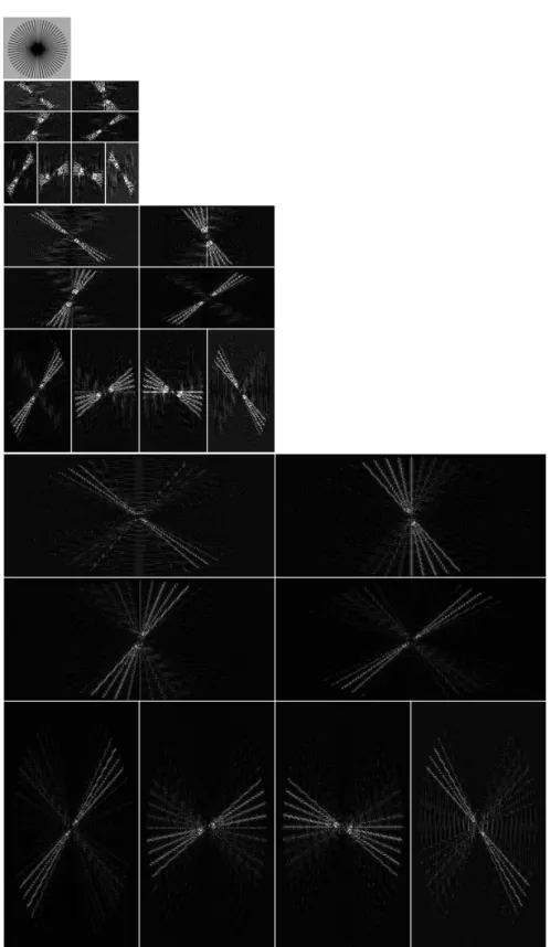
2.19 Steerable pyramid outputs of the fireworks pattern, for 3 scales . . 41
2.20 Steerable pyramid outputs of the zoneplate pattern, for 3 scales . 42
LIST OF FIGURES xii
2.22 LM Responses to fireworks pattern . . . 48
2.23 LM Responses to zoneplate pattern . . . 50
2.24 RFS Filters . . . 51
2.25 RFS Responses to fireworks pattern . . . 52
2.26 RFS Responses of zoneplate pattern . . . 53
2.27 MR8 Responses to fireworks pattern . . . 54
2.28 MR8 Responses to zoneplate pattern . . . 54
2.29 Highest % 2 Responses of real, imaginary and complex Gabor Fil-ters to fireworks pattern, for λ = 5.4, θ = π/8 . . . . 54
2.30 Real(left filter in each image) and imaginary(right filter in each im-age) Gabor Filters, for λ = [2.7, 4.1, 5.4] and θ = [π/8, 2π/8, . . . , π]. 56 2.31 Gabor Filter responses to fireworks pattern, for λ = [2.7, 4.1, 5.4] and θ = [π/8, 2π/8, . . . , π] . . . . 58
2.32 Gabor Filter responses to zoneplate pattern, for λ = [2.7, 4.1, 5.4] and θ = [π/8, 2π/8, . . . , π] . . . . 60
2.33 Immediate neighbours(d=1) of a pixel, corresponding offset values and corresponding angles . . . 61
2.34 Non-zero elements of GLCM of fireworks pattern, for d = 1, . . . , 4
and θ ={0◦, 45◦, 90◦, 135◦} . . . 62
2.35 Non-zero elements of GLCM of zoneplate pattern, for d = 1, . . . , 4
and θ ={0◦, 45◦, 90◦, 135◦} . . . 63
3.1 Example subsamples and average features of Arial bold, for various subsample sizes . . . 68
LIST OF FIGURES xiii
3.2 Mean recognition accuracies for each feature on datasets 1,2,3 . . 69
List of Tables
1.1 Average SNR values of English datasets three levels of noise . . . 5
2.1 Directional and rotated filters for θ ={0◦,±26.56◦,±45◦,±63.43◦, 90◦} 14
2.2 Time required for each feature to be extracted from a N×N image,
for N = [512, 1024, 2048] . . . . 64
2.3 Each entry is divided by the smallest entry in the column, for
N = [512, 1024, 2048] . . . . 64
3.1 Recognition rates of a classifier trained with features extracted
from 96x96 sized windows (using CWT features) . . . 67
3.2 Recognition rates(%) of the feature extraction algorithms on
Dataset 1 (English Printscreen texts). . . 70
3.3 Recognition rates(%) of the feature extraction algorithms on
Dataset 2 (English low noisy texts) . . . 71
3.4 Recognition rates(%) of the feature extraction algorithms on
Dataset 4 (English high noisy texts) . . . 72
3.5 Recognition rates(%) of the feature extraction algorithms on
LIST OF TABLES xv
3.6 Recognition rates(%) of the tested algorithms and comparisons
with [2] and [3] on Farsi texts. . . 74
3.7 Recognition accuracies of the tested algorithms and the method of
Ben Moussa et al. [4] on ALPH-REGIM database . . . 75
3.8 Recognition accuracies of each algorithm on Dataset 8 (Ottoman
scripts) . . . 76
4.1 10-fold cross-validation accuracies of each grade, for each feature . 79
5.1 Mean error in Stratum corneum thickness (µm) of each test stack
for each feature . . . 84
A.1 Confusion matrix of the optimal classifier trained with CWT
fea-tures in no-noise set (Dataset 1) . . . 95
A.2 Confusion matrix of the optimal classifier trained with contourlet
features in no-noise set (Dataset 1) . . . 96
A.3 Confusion matrix of the optimal classifier trained with curvelet
features in no-noise set (Dataset 1) . . . 97
A.4 Confusion matrix of the optimal classifier trained with dirfil3
fea-tures in no-noise set (Dataset 1) . . . 98
A.5 Confusion matrix of the optimal classifier trained with dirfil4
fea-tures in no-noise set (Dataset 1) . . . 99
A.6 Confusion matrix of the optimal classifier trained with gabor fea-tures in no-noise set (Dataset 1) . . . 100 A.7 Confusion matrix of the optimal classifier trained with LM features
LIST OF TABLES xvi
A.8 Confusion matrix of the optimal classifier trained with MR8 fea-tures in no-noise set (Dataset 1) . . . 102 A.9 Confusion matrix of the optimal classifier trained with pyramid
features in no-noise set (Dataset 1) . . . 103 A.10 Confusion matrix of the optimal classifier trained with CWT
fea-tures in low-noise set (Dataset 2) . . . 104 A.11 Confusion matrix of the optimal classifier trained with contourlet
features in low-noise set (Dataset 2) . . . 105 A.12 Confusion matrix of the optimal classifier trained with curvelet
features in low-noise set (Dataset 2) . . . 106 A.13 Confusion matrix of the optimal classifier trained with dirfil3
fea-tures in low-noise set (Dataset 2) . . . 107 A.14 Confusion matrix of the optimal classifier trained with dirfil4
fea-tures in low-noise set (Dataset 2) . . . 108 A.15 Confusion matrix of the optimal classifier trained with gabor
fea-tures in low-noise set (Dataset 2) . . . 109 A.16 Confusion matrix of the optimal classifier trained with LM features
in low-noise set (Dataset 2) . . . 110
A.17 Confusion matrix of the optimal classifier trained with MR8 fea-tures in low-noise set (Dataset 2) . . . 111 A.18 Confusion matrix of the optimal classifier trained with pyramid
features in low-noise set (Dataset 2) . . . 112 A.19 Confusion matrix of the optimal classifier trained with CWT
LIST OF TABLES xvii
A.20 Confusion matrix of the optimal classifier trained with contourlet features in high-noise set (Dataset 3) . . . 114 A.21 Confusion matrix of the optimal classifier trained with curvelet
features in high-noise set (Dataset 3) . . . 115 A.22 Confusion matrix of the optimal classifier trained with dirfil3
fea-tures in high-noise set (Dataset 3) . . . 116 A.23 Confusion matrix of the optimal classifier trained with dirfil4
fea-tures in high-noise set (Dataset 3) . . . 117 A.24 Confusion matrix of the optimal classifier trained with gabor
fea-tures in high-noise set (Dataset 3) . . . 118 A.25 Confusion matrix of the optimal classifier trained with LM features
in high-noise set (Dataset 3) . . . 119 A.26 Confusion matrix of the optimal classifier trained with MR8
fea-tures in high-noise set (Dataset 3) . . . 120 A.27 Confusion matrix of the optimal classifier trained with pyramid
features in high-noise set (Dataset 3) . . . 121 A.28 Confusion matrix of the optimal classifier trained with CWT
fea-tures in Chinese dataset . . . 122 A.29 Confusion matrix of the optimal classifier trained with contourlet
features in Chinese dataset . . . 123 A.30 Confusion matrix of the optimal classifier trained with curvelet
features in Chinese dataset . . . 124 A.31 Confusion matrix of the optimal classifier trained with dirfil3
LIST OF TABLES xviii
A.32 Confusion matrix of the optimal classifier trained with dirfil4 fea-tures in Chinese dataset . . . 126 A.33 Confusion matrix of the optimal classifier trained with gabor
fea-tures in Chinese dataset . . . 127 A.34 Confusion matrix of the optimal classifier trained with LM features
in Chinese dataset . . . 128
A.35 Confusion matrix of the optimal classifier trained with MR8 fea-tures in Chinese dataset . . . 129 A.36 Confusion matrix of the optimal classifier trained with pyramid
features in Chinese dataset . . . 130 A.37 Confusion matrix of the optimal classifier trained with CWT
fea-tures in Farsi set . . . 131
A.38 Confusion matrix of the optimal classifier trained with contourlet features in Farsi set . . . 132 A.39 Confusion matrix of the optimal classifier trained with curvelet
features in Farsi set . . . 133 A.40 Confusion matrix of the optimal classifier trained with dirfil3
fea-tures in Farsi set . . . 134
A.41 Confusion matrix of the optimal classifier trained with dirfil4
fea-tures in Farsi set . . . 135
A.42 Confusion matrix of the optimal classifier trained with gabor
fea-tures in Farsi set . . . 136
A.43 Confusion matrix of the optimal classifier trained with LM features in Farsi set . . . 137
LIST OF TABLES xix
A.44 Confusion matrix of the optimal classifier trained with MR8
fea-tures in Farsi set . . . 138
A.45 Confusion matrix of the optimal classifier trained with pyramid features in Farsi set . . . 139 A.46 Confusion matrix of the optimal classifier trained with CWT
fea-tures in ALPH-REGIM dataset . . . 140 A.47 Confusion matrix of the optimal classifier trained with contourlet
features in ALPH-REGIM dataset . . . 140 A.48 Confusion matrix of the optimal classifier trained with curvelet
features in ALPH-REGIM dataset . . . 140 A.49 Confusion matrix of the optimal classifier trained with dirfil3
fea-tures in ALPH-REGIM dataset . . . 141 A.50 Confusion matrix of the optimal classifier trained with dirfil4
fea-tures in ALPH-REGIM dataset . . . 141 A.51 Confusion matrix of the optimal classifier trained with gabor
fea-tures in ALPH-REGIM dataset . . . 141 A.52 Confusion matrix of the optimal classifier trained with LM features
in ALPH-REGIM dataset . . . 141
A.53 Confusion matrix of the optimal classifier trained with MR8 fea-tures in ALPH-REGIM dataset . . . 141 A.54 Confusion matrix of the optimal classifier trained with pyramid
Chapter 1
Introduction
Almost all images studied in classification problems regardless of area of appli-cation, have directional information embedded into its texture. In some cases this information create intra-class variance that needs to accounted for; or some-times direction stand as a discriminating feature. In any case, there is a need to extract the direction information. This gives rise to development of many different multi-scale directional feature extraction methods, such as curvelets [5], bandelets [6], wedgelets [7], steerable pyramids [8], directional wavelets [9], com-plex wavelets [10], directional filter banks [11], co-occurrence matrices [12],and Gabor filters [13]. There is no ’golden’ method that works the best in all areas of application. Each algorithm has its advantages and drawbacks. This thesis com-pares several directional feature extraction algorithms on several different image datasets with different areas of application and different modalities. Notice that we cover only the most widely used multi-scale directional image representation algorithms. Ref. [14] provides an excellent review article covering almost all of directional image analysis algorithms reported in the literature. However, these algorithms are not compared to each other in [14].
The thesis is organized as follows: The rest of this chapter is dedicated to definition of three distinct problems and explanation of related datasets used in this thesis: font recognition, follicular lymphoma grading, and stratum corneum thickness estimation. A brief literature survey and background information on
directional feature extraction methods are presented in Chapter 2. Compari-son of aforementioned algorithms on font recognition is presented in Chapter 3. Comparison of algorithms on follicular lymphoma grading and cancer cell line classification on microscopic images are presented in Chapter 4. Comparison of algorithms on stratum corneum thickness estimation on reflectance confocal mi-croscopy images will be presented in Chapter 5. Finally, Chapter 6 will conclude the thesis.
In this thesis we test the algorithms on images acquired with three different modalities. The datasets and modalities used in each problem is described:
1. Font Recognition
(a) Scanned text images
i. English Lorem Ipsum texts, A. Noise-free set
B. Low noise set C. High noise set
ii. Chinese Lorem Ipsum texts, iii. Persian Lorem Ipsum texts, iv. ALPH-REGIM database [15], and
v. Ottoman Scripts 2. Follicular Lymphoma Grading
(a) Light Microscope Images
3. Stratum Corneum Thickness Estimation (a) Reflectance Confocal Microscopy Images
1.1
Font Recognition Problem
Font recognition is an important issue in document analysis especially on multi-font documents [16, 2]. Besides its advantages in capturing the document layout, font recognition may also help to increase the performance of optical character recognition (OCR) systems by reducing the variability of shape and size of the characters to be recognized. Since it is intended to be used as a preprocessing stage, a good font recognition algorithm should be computationally as simple as possible in order not to introduce further overhead to overall OCR process.
Recently, a number of font recognition approaches were proposed in the lit-erature. Local features that usually refer to typographical information gained from parts of individual letters were utilized in [17, 18, 19]. Alternatively, global features refer to information extracted from entire words, lines, or pages, and mostly texture based features [20, 21, 22, 2, 16], such as Gabor filters [23, 24] or higher order moments [25, 26] were used, but some of this feature extraction algorithms are computationally complex, thus they introduce overhead.
Since local feature extraction relies on character segmentation, the document should be noise-free and scanned in high resolution. When Arabic or Farsi doc-uments with cursive scripts are considered, the change in character shape with location (i.e. isolated, initial, medial and final); and dots above or below the letters cause difficulties in character segmentation. Obviously, if it is desired to be used as a preprocessing stage, a font recognition algorithm should use global feature extraction.
Classification of handwriting calligraphy styles continues to be a challenging yet an important problem for paleographic analysis [27]. In classification of He-brew [28], Chinese [29], and Arabic [30] calligraphy, characters are used as the basic elements to extract the features. However, these methods heavily rely on preprocessing steps and they are prone to error.
Different styles have been used in different writings, such as books, letters, de-crees. Classification of Ottoman calligraphy styles would be an important step for categorization of large number of documents in archives. Furthermore, it could be used as an initial step for automatic transliteration. Ottoman is similar to Farsi and Arabic in the sense that it is written right to left, it is a cursive script, and the alphabets are similar. However, existing methods on Arabic and Farsi font recognition cannot be easily utilized for Ottoman calligraphy.Due to the late adoption of printing technology, a high percentage of scripts are hand-written resulting in intra-class variances much higher than printed fonts. Some of the documents are hundreds of years old and non-optimal storage conditions in Ottoman archives resulted in highly degraded documents. Moreover, in order not to damage the binding, books are scanned with their pages partially open, introducing non-uniform lighting.
To compare different methods with the state-of-the-art studies, we used avail-able datasets provided by other studies and generated artificial datasets. We used fonts used in [31] for English texts, fonts used in [23] for Chinese texts,and fonts used in [2] for Farsi texts. For Arabic, we used an available dataset prepared by [4]. We also constructed a new dataset for Ottoman by scanning pages from Ottoman documents written in different calligraphy styles.
1.1.1
Dataset 1: English Lorem Ipsum Texts
In order to test the noise performance of the algorithms, we created four different English datasets. The first set, named “Noise-free set”, consists of saved pages of English lorem ipsum texts typed in eight different typefaces (namely Arial, Bookman, Courier, Century Gothic, Comic Sans MS, Impact, Modern, Times New Roman), and in four emphases (regular, italic, bold, bold-italic) are directly converted to images. An example is presented in Figure 1.1-(a). The term “Noise-free set” here means no noise is introduced in generating or saving the texts, as texts are directly fed to the algorithms as images. This set is used for validation and comparison of algorithms in ideal case.
1.1.1 Noise-free 1.1.2 Low noise
1.1.3 High noise
Figure 1.1: Examples from English datasets
We also created noisy versions of the same texts by printing and scanning the pages in 200 dpi as done in [25], using a Gestetner MP 7500 printer/scanner. This introduced a small amount of noise to the images, hence the dataset created from these pages are named “Low noise set”.
Last English dataset is created by photocopying and scanning the texts 10 times in succession. This results in a clear degradation of image quality and introduced a large number of artifacts. Hence, this set is an approximation of a worn-out document. This set is named “High noise set”
These three datasets are used for comparisons with other studies in the liter-ature, and to understand the effect of algorithms and parameters. The average signal to noise ratio (SNR) values for each set is given in Table 1.1
Table 1.1: Average SNR values of English datasets three levels of noise
Set Average SNR
Low noise set 8.2487
Figure 1.2: Example of Chinese dataset, in SongTi italic
1.1.2
Dataset 2: Chinese Lorem Ipsum Texts
Since tested algorithms extract textural information which is not unique to any specific language, there are no limitations on the language or the alphabet. We show this advantage of our method, by testing it on Chinese texts. Four different emphases (italic, bold, bold-italic, regular) of six different typefaces (SongTi, KaiTi, HeiTi, FangSong, LiShu and YouYuan) that are used in [23] are used to construct this dataset. An example of the scanned pages of Chinese lorem ipsum texts is shown in Figure 1.2. This dataset is the Chinese equivalent of noise-free set (Dataset 1(a)).
1.1.3
Dataset 3: Farsi Lorem Ipsum Texts
Ottoman alphabet is similar in nature to Farsi alphabet, so we also tested our method on Farsi texts. To compare performance against Khosravi and Kabir’s [2] method, we tried to replicate the dataset used in [2]. The dataset consists of scanned pages of Farsi lorem ipsum paragraphs written in four different emphases (italic, bold, bold-italic, regular) of ten different typefaces: Homa, Lotus, Mitra, Nazanin, Tahoma, Times New Roman, Titr, Traffic, Yaghut, and Zar. Only regular and italic have been used for Titr, because bold emphasis is not available for that font. Examples of the set are shown in Figure 1.3.
1.3.1 Homa regular 1.3.2 Tahoma italic Figure 1.3: Examples of Farsi texts
1.1.4
Dataset 4: ALPH-REGIM Database
ALPH-REGIM Database1, constructed in [15], a is dataset for printed
Ara-bic scripts. The dataset consists of text snippets of various fonts, sizes and
lengths. We use ten typefaces which are also used in [15]: Ahsa, Andalus, Ara-bictransparant, Badr, Buryidah, Dammam, Hada, Kharj, Koufi and Naskh.
1.1.5
Dataset 5: Ottoman Scripts
Automatic classification of Ottoman calligraphy is relatively unstudied problem in font and calligraphy style recognition [32]. In order to show our algorithm can classify calligraphy styles as well as fonts, we generated a novel dataset from docu-ments written in Ottoman calligraphy by scanning 30 pages written in 5 different styles (divani, matbu, nesih, rika,talik). Examples are shown in Figure 1.4.
1.2
Follicular Lymphoma Grading Problem
Follicular Lymphoma(FL) is a group of malignancies of lymphocyte origin that arise from lymph nodes, spleen, and bone marrow in the lymphatic system in most
1.4.1 Divani 1.4.2 Matbu 1.4.3 Nesih
1.4.4 Rika 1.4.5 Talik
Figure 1.4: Example pages from different styles of Ottoman calligraphy. Images are cropped for space limitations
1.5.1 Grade 1 1.5.2 Grade 2 1.5.3 Grade 3 Figure 1.5: Example images for each of 3 grades of follicular lymphoma. cases and is the second most common non-Hodgkins lymphoma [33]. Character-istic of FL is the presence of a follicular or nodular pattern of growth presented by follicle center B cells consisting of centrocytes and centroblasts. World Health Organization’s (WHO) histological grading process of FL depends on the number of centroblasts counted within representative follicles, resulting in three grades with increasing severity [34]:
Grade 1 0-5 centroblasts(CBs) per high-power field (HPF) Grade 2 6-15 centroblasts per HPF
Grade 3 More than 15 centroblasts per HPF
Therefore, accurate grading of follicular lymphoma images is of course essen-tial to the optimal choice of treatment. One common way of grade FL images is an expert manually counting the centroblasts in an image, which is time consum-ing. Recently. Suhre proposed 2-level classification tree using sparsity-smoothed Bayesian classifier, and reported very high accuracies [35].
The dataset provided by [35] is also used in this thesis. The dataset consists of 90 images for each of 3 grades of Follicular Lymphoma.
1.3
Stratum Corneum Thickness Estimation
Problem
Thickness estimation of the stratum corneum (SC) is often required in pharmaco-logical, dermatological and cosmetological work. Reflectance confocal microscopy (RCM) is a non-invasive technique for high resolution imaging of cellular layers in skin. Although automated SC thickness estimation algorithms are available for other imaging modalities such as optical coherence tomography, multi-photon microscopy, and Raman-spectroscopy, RCM based SC measurements currently rely on manual visual analysis of images, which is subjective and variable.
Confocal Reflectance Microscopy is a relatively new modality for imaging the human skin in vivo[36]. Reflectance confocal microscopy works by detecting single back-scattered photon from the illuminated in-focus section through a pinhole-sized filter and rejecting light reflected from out-of-focus portions of the object. Laser beam is then scanned on the horizontal plane producing 2-dimensional pictures representing parallel sections of the skin. Confocal Scanning Laser Mi-croscopy enables the non-invasive imaging of skin structures with cellular-level
resolution (0.5−1.0µm in the lateral dimension and 4−5µm in the axial ones) to
a depth limited to 200 to 300µm, in relation to the wavelength of the employed laser-light, corresponding to the level of papillary dermis in normal skin. The dataset consists of seven 62-layer stacks covering 93µm of human skin acquired
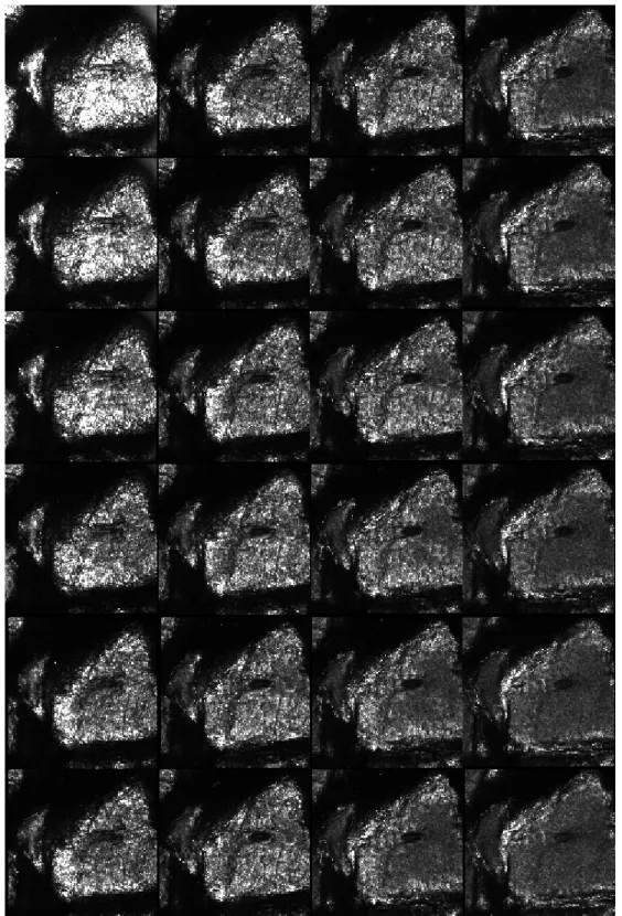
Figure 1.6: Example stack of confocal reflectance microscopy showing stratum corneum and stratum granulosum layers. Each consecutive image is 1.5µm apart.
Chapter 2
Background on Multi-scale
Directional Feature Extraction
Algorithms Studied in This
Thesis
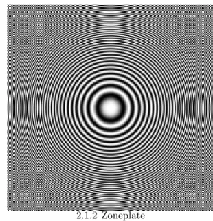
In this chapter, we will provide some background information on the algorithms used in this thesis. Algorithms are tested on two images to display their ad-vantages and shortcomings. These images are a fireworks pattern and zoneplate pattern, which are presented in Figure 2.1. Fireworks is used to test directional selectivity of algorithms, whereas zoneplate is used to test the algorithms ability to capture curved edges and gradual changes. In Section 2.9 we also compare the
time required for feature for a N × N image.
2.1
Directional Filtering
Directional filtering is a new framework developed in this thesis. In this
frame-work, we start with a given filter impulse response f0 with filter length N in
2.1.1 Fireworks 2.1.2 Zoneplate Figure 2.1: Test images: Fireworks and Zoneplate
To do so, we propose to create a set of filters obtained by rotating f0 along a set
of angles parameterized by θ.
Instead of rotating f0 by bilinear (or cubic) interpolation, we use the following
method: For a specific angle θ, we draw a line l going through origin (l : y =
tan θx) and determine the coefficients of the rotated filter fθ(i, j) proportional to
the length of the line segment within each pixel (i, j), which is denoted by |li,j|.
For odd N , f0(0) is exactly the center of rotation, therefore value of f0(0) does
not change in fθ(0, 0). Therefore we take line segment in origin pixel |l0,0| as
reference (|F G| in Figure 2.2(b)). For θ ≤ 45◦ , |l0,0| = cos θ1 , assuming each pixel
is of unit side. For each pixel in column j in the grid, we calculate the fθ(i, j) as
fθ(i, j) = f0(i)× |l|l0,0i,j||. This approach is also used in computerized tomography
[37].
Calculating the line segment |li,j| is straightforward. To rotate the filter for
θ ≤ 45◦ (which corresponds to Nv ≤ 1), we place f0 to the vertical center of a
N × N grid, where CX(i, j) and CY(i, j) are the coordinates of the center of cell
with horizontal index i = 0, . . . , N− 1, and vertical index j = 0, . . . , N − 1. Then
we construct a line l along the desired direction where the bisector of the line is the exact center of the grid (which is also the center of filter). For every cell
of the grid, we calculate the rotated filter coefficients as : fθ(i, j) = f0(i, j)×
max(0, 1− C(i, j) + l(Cx(i, j))). To rotate the filter for θ ≥ 45◦ we first rotate the
filter 90◦− θ then transpose f90◦−θ to get fθ. Note that this method of rotation
retains the DC response of the original filter, since ∑i,jfθ(i, j) =
∑
kf0(k).
Table 2.1: Directional and rotated filters for θ ={0◦,±26.56◦,±45◦,±63.43◦, 90◦}
Angle Directional Filter Rotated Filter
−63.43◦ 0 −0.0313 −0.0313 0 0 0 0 0 0 0 0 0 0 0 0 0 0.2813 0.2813 0 0 0 0 0 0 1 0 0 0 0 0 0 0.2813 0.2813 0 0 0 0 0 0 0 0 0 0 0 0 0 −0.0313 −0.0313 0 0 −0.01459 −0.03004 0 0 0 0 0 −0.00451 −0.01475 0.012539 0 0 0 0 0 0.204712 0.336475 0 0 0 0 0 0.084917 1 0.084917 0 0 0 0 0 0.336475 0.204712 0 0 0 0 0 0.012539 −0.01475 −0.00451 0 0 0 0 0 −0.03004 −0.01459 0 −45◦ −0.0625 0 0 0 0 0 0 0 0 0 0 0 0 0 0 0 0.5625 0 0 0 0 0 0 0 1 0 0 0 0 0 0 0 0.5625 0 0 0 0 0 0 0 0 0 0 0 0 0 0 0 −0.0625 0 −0.0085 0 0 0 0 0 −0.0085 −0.05178 −0.00222 0 0 0 0 0 −0.00222 0.329505 0.202284 0 0 0 0 0 0.202284 1 0.202284 0 0 0 0 0 0.202284 0.329505 −0.00222 0 0 0 0 0 −0.00222 −0.05178 −0.0085 0 0 0 0 0 −0.0085 0 −26.56◦ 0 0 0 0 0 0 0 −0.0313 0 0 0 0 0 0 −0.0313 0 0.2813 0 0 0 0 0 0 0.2813 1 0.2813 0 0 0 0 0 0 0.2813 0 −0.0313 0 0 0 0 0 0 −0.0313 0 0 0 0 0 0 0 0 0 0 0 0 0 0 −0.01459 −0.00451 0 0 0 0 0 −0.03004 −0.01475 0.204712 0.084917 0 0 0 0 0.012539 0.336475 1 0.336475 0.012539 0 0 0 0 0.084917 0.204712 −0.01475 −0.03004 0 0 0 0 0 −0.00451 −0.01459 0 0 0 0 0 0 0 0◦ 0 0 0 0 0 0 0 0 0 0 0 0 0 0 0 0 0 0 0 0 0 −0.0625 0 0.5625 1 0.5625 0 −0.0625 0 0 0 0 0 0 0 0 0 0 0 0 0 0 0 0 0 0 0 0 0 0 0 0 0 0 0 0 0 0 0 0 0 0 0 0 0 0 0 0 0 0 −0.0625 0 0.5625 1 0.5625 0 −0.0625 0 0 0 0 0 0 0 0 0 0 0 0 0 0 0 0 0 0 0 0 0 26.56◦ 0 0 0 0 0 0 0 0 0 0 0 0 0 −0.0313 0 0 0 0 0.2813 0 −0.0313 0 0 0.2813 1 0.2813 0 0 −0.0313 0 0.2813 0 0 0 0 −0.0313 0 0 0 0 0 0 0 0 0 0 0 0 0 0 0 0 0 0 0 0 0 0 0 0 0 −0.00451 −0.01459 0 0 0 0.084917 0.204712 −0.01475 −0.03004 0 0.012539 0.336475 1 0.336475 0.012539 0 −0.03004 −0.01475 0.204712 0.084917 0 0 0 −0.01459 −0.00451 0 0 0 0 0 0 0 0 0 0 0 0 45◦ 0 0 0 0 0 0 −0.0625 0 0 0 0 0 0 0 0 0 0 0 0.5625 0 0 0 0 0 1 0 0 0 0 0 0.5625 0 0 0 0 0 0 0 0 0 0 0 −0.0625 0 0 0 0 0 0 0 0 0 0 0 −0.0085 0 0 0 0 0 −0.00222 −0.05178 −0.0085 0 0 0 0.202284 0.329505 −0.00222 0 0 0 0.202284 1 0.202284 0 0 0 −0.00222 0.329505 0.202284 0 0 0 −0.0085 −0.05178 −0.00222 0 0 0 0 0 −0.0085 0 0 0 0 0 63.43◦ 0 0 0 0 −0.0313 −0.0313 0 0 0 0 0 0 0 0 0 0 0 0.2813 0.2813 0 0 0 0 0 1 0 0 0 0 0 0.2813 0.2813 0 0 0 0 0 0 0 0 0 0 0 −0.0313 −0.0313 0 0 0 0 0 0 0 0 −0.03004 −0.01459 0 0 0 0 0.012539 −0.01475 −0.00451 0 0 0 0 0.336475 0.204712 0 0 0 0 0.084917 1 0.084917 0 0 0 0 0.204712 0.336475 0 0 0 0 −0.00451 −0.01475 0.012539 0 0 0 0 −0.01459 −0.03004 0 0 0 0 90◦ 0 0 0 −0.0625 0 0 0 0 0 0 0 0 0 0 0 0 0 0.5625 0 0 0 0 0 0 1 0 0 0 0 0 0 0.5625 0 0 0 0 0 0 0 0 0 0 0 0 0 −0.0625 0 0 0 0 0 0 −0.0625 0 0 0 0 0 0 0 0 0 0 0 0 0 0.5625 0 0 0 0 0 0 1 0 0 0 0 0 0 0.5625 0 0 0 0 0 0 0 0 0 0 0 0 0 −0.0625 0 0 0
This method imposes a lower bound on θ, since at the line should cross at
2.2.1 f0(i, j) 2.2.2 Line θ = arctan 1/2 = 26.565◦
2.2.3 Lengths of line segments in each pixel 2.2.4 Resulting f26.56◦ Figure 2.2: Filter rotation process for Lagrange a trois filter
have side l, this bound is calculated as follows: tan(θ)[Cx( N − 1 2 , 0) + l/2] ≥ l 2 (2.1) tan(θ) ≥ 1 2Cx(N−12 , 0) + 1 (2.2) tan(θ) ≥ 1 N (2.3) θ ≥ arctan( 1 N) (2.4)
Resulting filters form a directional filter bank are shown in the first row of Table 2.1. These directional filters are used in a multi-resolution framework for feature extraction. For the first scale, directional images can be extracted by convolving the input image with this filter bank. Mean and standard of these directional images are used as the directional feature values of the image (other statistics, or the image itself can also be used). To obtain direction feature values at lower scales, the original image is low-pass filtered and decimated by a factor of two horizontally and vertically and a low-low sub-image is obtained. Since downsampling is a shift variant process, we also introduce a half-sample delay before downsampling. To implement this, we downsample two shifted versions of
input image (corresponding to (∆x, ∆y) ={(0, 0), (1, 1)}), pass two downsampled
images from our directional filter bank, and fuse the outputs to construct one output image per filter in directional filter bank. Fusing method used in thesis is simply taking square of images, summing them, and taking the square root of the sum.
A variant of this multi-scale filtering framework uses four shifted versions
in-stead of two (corresponding to (∆x, ∆y) ={(0, 0), (1, 0), (0, 1), (1, 1)}). Although
this increases the accuracy by average 1%, it also doubles the computational complexity. This speed vs. accuracy trade-off should be evaluated for potential applications.
The lowpass filter used in downsampling f0 can be the corresponding lowpass
filter of a wavelet filter bank. If f0 is chosen as such, or it can be a simple
2.3.1 Directional Filter Frequency Response(θ =−63.43◦)
2.3.2 Rotated Filter Frequency Response(θ =−63.43◦)
2.3.3 Directional Filter Frequency Response(θ =−45◦)
2.3.4 Rotated Filter Frequency Response(θ =−45◦)
2.3.5 Directional Filter Frequency Response(θ =−26.56◦)
2.3.6 Rotated Filter Frequency Response(θ =− − 26.56◦)
2.3.7 Directional Filter Frequency Response(θ = 0◦)
2.3.8 Rotated Filter Frequency Response(θ =−0◦)
2.3.9 Directional Filter Frequency Response(θ = 26.56◦)
2.3.10 Rotated Filter Frequency Response(θ = 26.56◦)
2.3.11 Directional Filter Frequency Response(θ = 45◦)
2.3.12 Rotated Filter Frequency Response(θ = 45◦)
2.3.13 Directional Filter Frequency Response(θ = 63.43◦)
2.3.14 Rotated Filter Frequency Response(θ = 63.43◦)
2.3.15 Directional Filter Frequency Response(θ = 90◦)
2.3.16 Rotated Filter Frequency Response(θ = 90◦)
Figure 2.3: Frequency responses of directional and rotated filters, for θ =
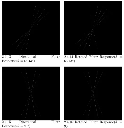
2.4.1 Directional Filter Response(θ =
−63.43◦) 2.4.2 Rotated Filter Response(θ =−63.43◦)
2.4.3 Directional Filter Response(θ =
−45◦) 2.4.4 Rotated Filter Response(θ =−45◦)
2.4.5 Directional Filter Response(θ =
2.4.7 Directional Filter Response(θ = 0◦)
2.4.8 Rotated Filter Response(θ = −0◦)
2.4.9 Directional Filter Response(θ = 26.56◦)
2.4.10 Rotated Filter Response(θ = 26.56◦)
2.4.11 Directional Filter
Response(θ = 45◦)
2.4.12 Rotated Filter Response(θ = 45◦)
2.4.13 Directional Filter Response(θ = 63.43◦)
2.4.14 Rotated Filter Response(θ = 63.43◦)
2.4.15 Directional Filter
Response(θ = 90◦)
2.4.16 Rotated Filter Response(θ = 90◦)
Figure 2.4: Largest %2 Responses of directional and rotated filters on fireworks
Figure 2.5: Image flowchart directional filtering framework
the second level directional subimages and corresponding feature values. This process can be repeated several times depending on the nature of input images. The filtering flow diagram is shown in Figure 2.5.
In our experiments, we use two different directional filters, both in 3 scales,
θ = {0◦,±26.56◦,±45◦,±63.43◦, 90◦} and lowpass filter is halfband filter fl =
[0.25 0.5 0.25]. For one filter bank we use Lagrange `a trous filter [38]: f0 =
[−0.0625 0 0.5625 1 0.5625 0 − 0.0625] and other uses Kingsburys 8th order
q-shift analysis filter [39]: f0 = [−0.0808 0 0.4155 −0.5376 0.1653 0.0624 0 −0.0248]
2.2
Complex Wavelet Transform
Complex wavelet transform(CWT) is developed by Kingsbury as an improve-ment over shortcomings of the discrete wavelet transform (DWT). DWT for 2-dimensional (2-D) signals can be implemented using two stages of filtering at each level: first, rows of the image are filtered to generate a pair of horizontal lowpass and highpass images, and then columns of these images are filtered to produce four sub-images.
However, as [40] states, there are two fundamental problems with real DWT that makes it unfeasible to model textural features with. First one is the shift
2.6.1 Level 1, (θ = 0◦) 2.6.2 Level 1, (θ = 90◦) 2.6.3 Level 1, (θ = 45◦) 2.6.4 Level 1, (θ = −45◦) 2.6.5 Level 1, (θ =
−63.43◦) 2.6.6 Level 1, (θ =63.43◦) 2.6.7 Level 1, (θ =−26.56◦) 2.6.8 Level 1, (θ =26.56◦)
2.6.9 Level 2, (θ =
−0◦) 2.6.10(θ = 90◦Level) 2, 2.6.11(θ = 45◦Level) 2, 2.6.12(θ =−45Level◦) 2,
2.6.13 Level 2, (θ =−63.43◦) 2.6.14 Level 2, (θ = 63.43◦) 2.6.15 Level 2, (θ =−26.56◦) 2.6.16 Level 2, (θ = 26.56◦) 2.6.17 Level 3, (θ = 0◦) 2.6.18 Level 3, (θ = 90◦) 2.6.19 Level 3, (θ = 45◦) 2.6.20 Level 3, (θ =−45◦) 2.6.21 Level 3, (θ =−63.43◦) 2.6.22 Level 3, (θ = 63.43◦) 2.6.23 Level 3, (θ =−26.56◦) 2.6.24 Level 3, (θ = 26.56◦) Figure 2.6: Directional Filter Responses of zoneplate pattern
variance. Note that implementation of DWT is maximally decimated, total out-put sample size is equal to the inout-put size for each level due to decimation at each level. This provides zero redundancy, however it also causes aliasing and results in shift variance. The other problem is poor directional selectivity. Since both highpass row filters and highpass column filters in DWT are real, their spectrum are symmetric. Therefore Lo-Hi and Hi-Lo filters select high frequencies in both positive and negative directions in their corresponding orientations (Hi-Lo filters select horizontal frequencies, Lo-Hi filters select vertical frequencies). Hi-Hi filter however, selects diagonal edges with both positive and negative gradients, due to having passbands in all four corners of the frequency plane. Output of Hi-Hi
fil-ter cannot separate +45◦ diagonal edges from−45◦ diagonal edges; which causes
poor directional selectivity [41]. This phenomenon can be seen clearly from the impulse responses in figure 2.7
As a solution, Kingsbury in [40] proposes dual-tree complex wavelet transform (DT-CWT), which is almost shift invariant, directionally selective, has perfect reconstruction, introduces minimal redundancy (4:1 for 2D signals) and achieves order-N computation. [40]
Filter selection is a critical issue and there are many papers on designing filters with suitable properties for wavelet transform. Following 6-tap filter designed in [39] and Farras filters [42] are used in our implementation:
Lop[n] = [0,−0.0884, 0.0884, 0.6959, 0.6959, 0.0884, −0.0884, 0.0112, 0.0112] (2.5) Hip[n] = [0.0112, 0.0112,−0.0884, 0.0884, 0.6959, 0.6959, 0.0884, −0.0884, 0, 0] (2.6) Lo[n] = [0.0351, 0,−0.0883, 0.2339, 0.7603, 0.5875, 0, −0.1143, 0, 0] (2.7) Hi[n] = [0, 0,−0.1143, 0, 0.5875, 0.7603, 0.2339, −0.0883, 0, 0.0351] (2.8)
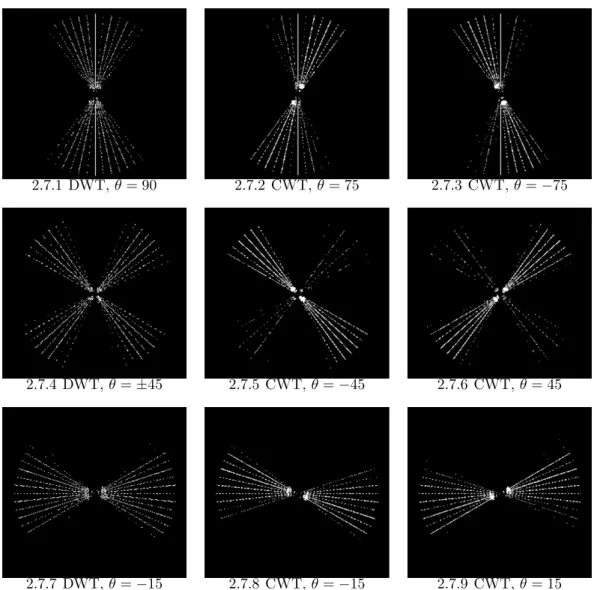
2.7.1 DWT, θ = 90 2.7.2 CWT, θ = 75 2.7.3 CWT, θ =−75
2.7.4 DWT, θ =±45 2.7.5 CWT, θ =−45 2.7.6 CWT, θ = 45
2.7.7 DWT, θ =−15 2.7.8 CWT, θ =−15 2.7.9 CWT, θ = 15
Figure 2.7: Top %2 responses of DWT (left column) and CWT(center and right columns) to fireworks pattern for at level 1
parts of the filters can we calculated by reversing and taking the negative of each respective filter.
Since DT-CWT produces output images with different size at each tree level due to decimation, and these sizes depend on input image size, it is not feasible
to use output images of DT-CWT directly. Instead we are using mean and
variance of the absolute value of outputs of 3 level complex wavelet tree. We have tried several levels, and found that the recognition rate does not increase noticeably after 3rd level. We have also tried taking mean and variance of real and imaginary parts of output images separately and concatenating them, but it gave poorer performance than the absolute values. Overall, our feature vector includes means and variances of 18 images (6 outputs for each level), resulting in
a 36-element feature vector1.
2.8.1 θ = 75◦ 2.8.2 θ =−45◦ 2.8.3 θ =−15◦ 2.8.4 θ = 15◦ 2.8.5 θ = 45◦ 2.8.6 θ = 75◦ 2.8.7 θ =−75◦ 2.8.8 θ =−45◦ 2.8.9 θ =−15◦ 2.8.10 θ = 15◦ 2.8.11 θ = 45◦ 2.8.12 θ = 75◦ Figure 2.8: 2D Impulse responses of CWT at level 4(top row:real, bottom row:imaginary)
2.3
Curvelet Transform
The problem in Figure 2.10 is the main motivation behind curvelets. Curvelets are first introduced in 1999 [43] and revised in 2003 [44], both by Candes and
1DT-CWT implementation given in http://eeweb.poly.edu/iselesni/WaveletSoftware/index.html is used in this thesis.
2.9.1 Level 1, θ =−75 2.9.2 Level 2, θ =−75 2.9.3 Level 3, θ =−75
2.9.4 Level 1, θ =−45 2.9.5 Level 2, θ =−45 2.9.6 Level 3, θ =−45
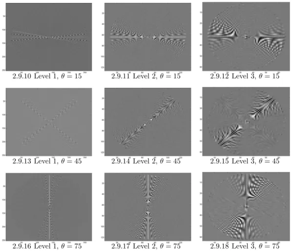
2.9.10 Level 1, θ = 15 2.9.11 Level 2, θ = 15 2.9.12 Level 3, θ = 15
2.9.13 Level 1, θ = 45 2.9.14 Level 2, θ = 45 2.9.15 Level 3, θ = 45
2.9.16 Level 1, θ = 75 2.9.17 Level 2, θ = 75 2.9.18 Level 3, θ = 75 Figure 2.9: Complex Wavelet Transform of the fireworks pattern, for 3 scales and
2.10.1 Level 1, θ =−75 2.10.2 Level 2, θ =−75 2.10.3 Level 3, θ =−75
2.10.4 Level 1, θ =−45 2.10.5 Level 2, θ =−45 2.10.6 Level 3, θ =−45
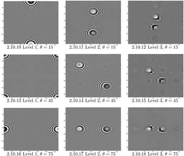
2.10.10 Level 1, θ = 15 2.10.11 Level 2, θ = 15 2.10.12 Level 3, θ = 15
2.10.13 Level 1, θ = 45 2.10.14 Level 2, θ = 45 2.10.15 Level 3, θ = 45
2.10.16 Level 1, θ = 75 2.10.17 Level 2, θ = 75 2.10.18 Level 3, θ = 75 Figure 2.10: Complex Wavelet Transform of the zoneplate pattern, for 3 scales
Donoho. The original curvelets are obtained by filtering an input image into band-pass images then applying windowed Ridgelet transform [45] in each bandband-pass image. The motivation for this is that by smooth windowing, segments of smooth curves with would look straight in subimages, hence they can be captured by a local ridgelet transform (Ridgelets are designed for efficiently capturing straight lines.) Curvelet transform is an improvement over wavelets, due to some of its properties which regular (or complex) wavelets are lacking. These are optimally sparse representation of object with edges, optimal sparse representation of wave propagators, and optimal image reconstruction in severely ill-posed problems.
Revised version of the curvelets does not utilize ridgelets. First, the frequency space is divided into dyadic annuli based on concentric squares, and each annulus is divided into trapezoidal regions. The redesigned version can be implemented by two different ways: Unequispaced FFTs or wrapping. Although each method calculate transform coefficients via different ways, computational complexity is
O(n2log n) for n× n image for both methods. In this thesis wrapping method is
used. A curvelet atom with scale s, orientation θ ∈ [0, π), position y ∈ [0, 1]2 is
defined as
ϕs,y,θ(x) = ϕs(R−10 (x− y)), (2.9)
where ϕs(x) ≈ s−3/4ϕ(s−1/2x1, s−1x2) is approximately a parabolic stretch of
a curvelet function ϕ with vanishing moments in vertical direction. At scale s, a curvelet atom is thus a needle oriented in the direction θ whose envelope is a
specified ridge of effective length s1/2 and width s, and which displays an
oscil-latory behavior transverse to the ridge. Hence, the curvelet atoms benefit from
anisotropic (more specifically, parabolic) scaling property width = length2 which
is a major departure from oriented wavelets. It follows from this property in
fre-quency domain that, a curvelet atom with width 2−2j have 2j orientations, that is
#orientations = √1
scale. It is clear to see from this relation that number of
orien-tations double at every other scale, which gives curvelets exceptional directional selectivity. The curvelet transform of fireworks pattern and zoneplate pattern can be seen in Figures 2.12 and 2.13, Respectively. When compared with CWT of
Figure 2.11: Spectral Decomposition of the curvelet transform, in frequency do-main. Notice the anisotropic scaling in frequency plane, and increasing angular resolution in finer scales. angular resolution doubles every other scale.
zoneplate pattern (Figure 2.10, it is clear that curvelets can capture edges with high accuracy.
2.4
Contourlet Transform
Contourlets are developed by Do and Vetterli [1] after the success of Curvelets. Contourlets can be considered as a low-redundancy discrete approximation of curvelets. They are designed in the spatial domain (instead of frequency plane as in curvelets) aiming at a close-to-critical directional representation. Their construction is based on Laplacian pyramid. The low pass part of the pyramid is further decomposed with. Each difference image obtained from the pyramid is subject to directional filter banks. A contourlet decompositions of fireworks and zoneplate patterns are illustrated in Figure 2.15 and 2.16. The contourlet transform is overcomplete by a factor of 4/3, which is inherited from the pyramidal framework. Its approximation rate is similar to that of curvelets.
Figure 2.14: Signal flow diagram for one level of the contourlet transform.(Taken from [1])
We use PKVA filters designed in [46] for both pyramid and directional filtering:
g[n] = [−0.0144, 0.0272, −0.0526, 0.0972, −0.1930,
0.6300, 0.6300,−0.1930, 0.0972, −0.0526, 0.0272, −0.0144]
2.5
Steerable Pyramids
Steerability theory is a very powerful theory that states, if a filter satisfies certain conditions, response of this filter along any orientation can be calculated by linear combination of output of row filtering and and column filtering with the same filter. In order to calculate filter response along several orientations, one simply calculates basis filter responses once then changes weights of combination to get the responses at each direction [47]. This reduces the computational workload substantially.
Figure 2.17: System diagram for radial decomposition of steerable pyramid. ‘steerable pyramids’. Working principle of steerable pyramids is divided into 2 parts: radial decomposition and angular decomposition. Angular decomposition uses the aforementioned steerable filter scheme and radial decomposition uses
pyramid scheme. Pyramidal scheme for radial decomposition can be seen in
Figure 2.5. Hollow circles correspond to transform coefficients, and filled circle correspond to the recursive block enclosed by dashed lines.
Pyramid scheme introduces its own constraints for filters in Figure 2.5 in addition to the steerability criteria. Method for designing filters satisfying these criteria is given in [48]. ‘sp5’ filter set designed with this method is used in this thesis.
When all constraints are satisfied, steerable pyramids are self-inverting, have no aliasing in subbands, and have flexible rotated orientation bands and perfect reconstruction ability, which makes it superior to other multi-scale representations such as Laplacian pyramids and dyadic quadratic mirror filters/wavelets [8]. As a trade-off, it is overcomplete by a factor of 4k/3 (where k is the number of orientation bands), which is highly redundant.
Steerable pyramid implementation of [8] are used in this thesis. Steerable pyramid outputs for fireworks and zoneplate patterns are presented in Figure 2.19 and 2.20.
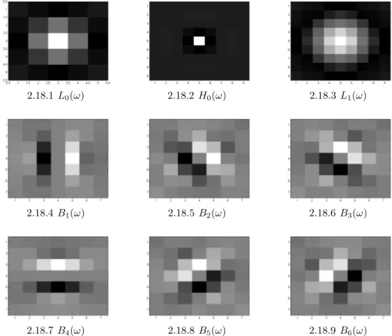
2.18.1 L0(ω) 2.18.2 H0(ω) 2.18.3 L1(ω)
2.18.4 B1(ω) 2.18.5 B2(ω) 2.18.6 B3(ω)
2.18.7 B4(ω) 2.18.8 B5(ω) 2.18.9 B6(ω)
Figure 2.18: Filter set used for scale and angular decomposition in steerable pyramid scheme
2.6
Texton Filters
Textons are introduced by Julesz in 1981, as ”the putative units of pre-attentive human texture perception” [49]. He described them as simple binary line segment stimulioriented segments, crossings and terminators, but did not provide an op-erational definition for gray-level images. Subsequently, texton theory fell into disfavor as a model of human texture discrimination as accounts based on spatial filtering with orientation and scale-selective mechanisms that could be applied to arbitrary gray-level images became popular. The term is reinvented in 1999 by Malik et. al. as clustered responses of an image to a filter bank [50]. They argue that the response to oriented odd-symmetric filter is not discriminative enough that visual cues such as edges, bars, or corners cannot be associated with the output of a single filter. Rather it is the characteristic of the outputs over scales, orientations and order of the filter that gives the relevant information. Following this logic, they consider outputs of these filters as points in a high dimensional space and try to find common characteristics for each class, via clustering. They define the centroid of resulting clusters, as textons. It turns out that textons do tend to correspond to visual cues such as oriented bars, terminators, etc. in an image. They propose that one can construct a texton dictionary by processing a large number of natural images, or we could find them adaptively in windows of images. In each case the K-means technique can be used. By mapping each pixel to the texton nearest to its vector of filter response
There are a number of filter banks constructed for texton formation that are multi-scale and direction-sensitive. Two of these, which are used in this thesis are small Leung-Malik (LMS) filter bank and Maximum Response 8 (MR8) filter bank. LM Filters are multi scale, multi orientation filter bank with 48 filters. It consists of first and second derivatives of Gaussians at 6 orientations and 3 scales making a total of 36; 8 Laplacian of Gaussian (LOG) filters; and 4 Gaussians. In
LMS, the filters occur at basic scales σ = {1,√2, 2, 2√2}. The first and second
derivative filters occur at the first three scales with an elongation factor of 3 (i.e.
σx = σ and σx = 3σ). The Gaussians occur at the four basic scales while the
fireworks pattern are shown in Figures 2.21 and 2.22, respectively.
The root filter set (RFS) filter bank is shown in Figure 2.24 and consists of a Gaussian and a LoG both with σ = 10 pixels, an edge filter at 3 scales:
(σx, σy) = (1, 3), (2, 6), (4, 12) and a bar filter at same scales [52]. The latter two
filters are oriented, an as in LM occur at 6 orientations at each scale. In order to reduce number of dimensions, Maximum Response (MR8) filter bank is intro-duced consists of 38 filters but only 8 responses. The filter bank contains filters at multiple orientations but their outputs are ‘collapsed’ by recording only the max-imum filter response across all orientations. This achieves rotation invariance. Measuring only the maximum response across orientations reduce the number of responses from 38 (6 orientations at 3 scales for 2 filters, plus 2 isotropic) to 8 (3 scales for 2 filters, plus 2 isotropic). An advantage of MR8 filter bank is that it can be applied using fast anisotropic Gaussian filtering [53], which results in significant decrease in computation time (see Table 2.2). The responses of RFS and MR8 filter banks to fireworks pattern can be seen in Figures 2.25 and 2.27, respectively. Although the MR8 filters is much faster than RFS filters, they display no directional selectivity.
2.7
Gabor Filters
2D Gabor filter are proposed by Daugman to model the response of direction sensitive simple cells in visual cortex [54]:
G(x, y) = 1 2πσβe −π[(x−x0)2 σ2 + (y−y0)2 β2 ]ei[ξ0x+ν0y] (2.10)
where (x0, y0) is the center of receptive field in spatial domain, (ξ0, ν0) is the
optimal spatial frequency of the filter in frequency domain, and (σ, β) are the standard deviations of the Gaussian function in x and y, respectively. Gabor function can be seen as a product of an elliptical Gaussian(first exponential in 2.10) and a complex planar wave(second exponential in 2.10).
Figure 2.21: LM Filters
Instead of 2.10, slightly different parametrization is used in [55]:
gλ,θ,ϕ,σ,γ(x, y) = exp(− x′2+ γ2y′2 2σ2 ) cos(2π x′ λ + ϕ) (2.11) x′ = (x− ϵ) cos θ + (y − ν) sin θ y′ = (x− ϵ) sin θ + (y − ν) cos θ
where (ϵ, ν) is the center of filter in spatial domain, σ is the standard deviation of the Gaussian, γ is the spatial aspect ratio of the filter a, ϕ is the phase offset,
θ is the orientation of the filter and λ is the wavelength of plane wave. Note
that 2.11 corresponds to the real part of the reparametrized 2D complex Gabor
function: gλ,θ,ϕ,σ,γ(x, y) = exp(−x′2+γ2σ22y′2) exp(i[2π
x′
λ + ϕ])
Parametrization of 2.11 will be used throughout this thesis. Since Gabor filters can be complex, we must choose which filter output to use: convolve the image with real part, imaginary part, or convolve it with both filters and fuse two outputs using absolute value. Figure 2.29 shows the highest % 2 values of the three outputs, λ = 5.4, θ = π/8. Output of complex filter is clearly more concentrated along the desired direction, whereas outputs of real and imaginary filters spread to adjoining angles. Therefore, although it doubles the computation time (due to doubling the number of convolutions), we choose to use the output
Figure 2.22: LM Responses to fireworks pattern of the complex filter. Resulting filter output is :
Y = abs(I∗ real(gλ,θ,ϕ,σ,γ) + i[I∗ imag(gλ,θ,ϕ,σ,γ)]) (2.12)
gλ,θ,ϕ,σ,γ(x, y) = exp(− x′2+ γ2y′2 2σ2 ) exp(i[2π x′ λ + ϕ]) (2.13) x′ = (x− ϵ) cos θ + (y − ν) sin θ y′ = (x− ϵ) sin θ + (y − ν) cos θ
Figures 2.30, 2.31 and 2.32 show the Gabor filters used in this thesis, and their responses to the fireworks and zoeplate pattern, respectively.
It has been found that spatial aspect ratio is limited in the range 0.23 < γ < 0.92 [56]. In this thesis, we choose γ = 0.5. For rest of the parameters, we choose parameters as in [31]: σ = 0.56, λ = [2.7, 4.1, 5.4] and θ = [π/8, 2π/8, . . . , π]. Values in Table 2.2 are measured with these parameters.
Figure 2.23: LM Responses to zoneplate pattern
2.8
Gray Level Co-Occurrence Matrices
Gray level co-occurrence matrices are first proposed as ‘gray-tone spatial depen-dence matrices’ by Haralick et. al.[12], to extract the spatial relationship which ne gray tones in image I have with one another. Haralick proposes that this
texture-content information can be specified by matrix of relative frequencies Pij
with two neighbouring cells separated by distance d occur on the image with one in gray tone i and other in gray tone j. Assume for a rectangular gray level
image with Nx horizontal pixels and Ny vertical pixels, so that the whole spatial
domain can be spanned by product of Lx = 1, . . . Nx and Ly = 1, . . . Ny.
More-over, assume that the image is quantized to Nθ levels. Then Pij for angles can
Figure 2.27: MR8 Responses to fireworks pattern
Figure 2.28: MR8 Responses to zoneplate pattern
2.29.1 Real 2.29.2 Imaginary 2.29.3 Complex
Figure 2.29: Highest % 2 Responses of real, imaginary and complex Gabor Filters to fireworks pattern, for λ = 5.4, θ = π/8
2.30.1 λ = 2.7, θ = π/8 2.30.2 λ = 4.1, θ = π/8 2.30.3 λ = 5.4, θ = π/8
2.30.4 λ = 2.7, θ = 2π/8 2.30.5 λ = 4.1, θ = 2π/8 2.30.6 λ = 5.4, θ = 2π/8
2.30.7 λ = 2.7, θ = 3π/8 2.30.8 λ = 4.1, θ = 3π/8 2.30.9 λ = 5.4, θ = 3π/8
2.30.13 λ = 2.7, θ = 5π/8 2.30.14 λ = 4.1, θ = 5π/8 2.30.15 λ = 5.4, θ = 5π/8
2.30.16 λ = 2.7, θ = 6π/8 2.30.17 λ = 4.1, θ = 6π/8 2.30.18 λ = 5.4, θ = 6π/8
2.30.19 λ = 2.7, θ = 7π/8 2.30.20 λ = 4.1, θ = 7π/8 2.30.21 λ = 5.4, θ = 7π/8
2.30.22 λ = 2.7, θ = π 2.30.23 λ = 4.1, θ = π 2.30.24 λ = 5.4, θ = π Figure 2.30: Real(left filter in each image) and imaginary(right filter in each image) Gabor Filters, for λ = [2.7, 4.1, 5.4] and θ = [π/8, 2π/8, . . . , π].
2.31.1 λ = 2.7, θ = π/8 2.31.2 λ = 4.1, θ = π/8 2.31.3 λ = 5.4, θ = π/8
2.31.4 λ = 2.7, θ = 2π/8 2.31.5 λ = 4.1, θ = 2π/8 2.31.6 λ = 5.4, θ = 2π/8
2.31.7 λ = 2.7, θ = 3π/8 2.31.8 λ = 4.1, θ = 3π/8 2.31.9 λ = 5.4, θ = 3π/8

![Figure 2.14: Signal flow diagram for one level of the contourlet transform.(Taken from [1])](https://thumb-eu.123doks.com/thumbv2/9libnet/5640392.112170/55.892.211.735.201.475/figure-signal-flow-diagram-level-contourlet-transform-taken.webp)