Efficient market hypothesis and comovement among emerging markets

EFFICIENT MARKET HYPOTHESIS AND COMOVEMENT

AMONG EMERGING MARKETS

ETKİN PİYASA HİPOTEZİ VE GELİŞMEKTE OLAN PİYASALARIN BİRLİKTE HAREKETİ

Oktay TAŞ 

oktay.tas@itu.edu.tr

Kaya TOKMAKÇIOĞLU 

tokmakcioglu@itu.edu.tr

ABSTRACT: The main purpose of this study is to investigate stock market

cointegration from the market efficiency perspective. Therefore, eleven emerging stock market indices are tested by using weekly data for the period of January 1998-December 2008 and for the sub period of January 2002-1998-December 2008. Comovement among the emerging market countries was analyzed through Johansen cointegration test. The existence of two cointegrating vectors has been found at 5% significance level. However, the firm evidence against the market efficiency could not be established because of the low explanatory power of the results generated from the vector error correction model.

Keywords: Efficient Market Hypothesis; Unit Root; Johansen Cointegration Test;

Vector Error Correction Model

JEL Classification: G14; G15

ÖZET: Bu çalışmanın amacı hisse senedi piyasaları eşbütünleşimini etkin pazar pespektifinden araştırmaktır. Bu bağlamda 11 gelişmekte olan piyasanın Ocak 1998-Aralık 2008 ve Ocak 2002-Aralık 2008 dönemli haftalık verileri test edilmiştir. Gelişmekte olan ülke piyasalarının birlikte hareketi Johansen eşbütünleşim testi ile incelenmiş ve %5 anlamlılık düzeyinde iki eşbütünleşim vektörü bulunmuştur. Buna rağmen vektör hata düzeltme modelinin açıklama gücünün düşük olmasından dolayı piyasa ekinliğine karşı kesin bir bulgu ortaya konulamamıştır.

Anahtar Kelimeler: Etkin Piyasa Hipotezi; Birim Kök; Johansen Eşbütünleşim Testi; Vektör Hata Düzeltme Modeli

JEL Sınıflamaları: G14; G15

Introduction

The technological developments, the increase in the rapidity in and the facilities of communication, the economic liberalism, the rise of international trade have formed the dynamic, what we now know as, globalism. The natural result of this is the integration among the economies. International investors need to understand the forces behind the interdependenceof emerging stock markets in order to realize the potential risks and rewards of global diversification. Likewise, policy-makers need to understand the driving forces behind emerging stock market interdependence, since from their point of view, contagion means irrational capital flows, especially capital outflows when capital is needed the most. As a matter of fact, the rise in comovement can be considered as a kind of information transfer between globalized economies. As it happened with every dynamic before, comovement attracts the

interest of the researchers which calls for an examination of the factors that influence the relationships and dynamic linkages between emerging stock markets. Such an understanding will provide a better grasp of the functioning of the emerging stock markets. As it is argued in the literature, the change in prices in the light of new information in the market and its random movement has been taken as a basis in all Efficient Market Hypothesis evaluations. If the adjustments in price are slow in comparison with the new information in the market, the asset prices will not reflect that information. If the adjustments in pricing are more or less than the norm, some investors would have an advantage over the other investors. The non-random movement in prices also leads to a violation of EMH as the investors, who can notice it, would have a considerable amount of profit.

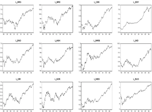
Croci (2003) shows that one of the most important results of comovement is the decline in the importance of diversification on a country basis and an increase in the importance of the diversification on a sectoral basis. It emphasizes an essential point in the portfolio management. Comovement is important according to the Efficient Market Hypothesis. Cerny (2004) points out to the fact that the information transition rate between the markets determines the compatibility rate of the prices which is crucial for the information expressivity. The interaction between the financial markets is increasing in these dynamics. Naturally, the markets began to have tendency to run parallel to each other. Figure 1 shows a general outlook on the rate of comovement in the last nine years.

Figure 1. The logarithmic index graphics of the emerging markets (98-08)

For example, the data support the fact that index movements are random to each other when we analyze the stock index in Turkey. To put it more clearly, it cannot be denied that index movement is random. The same results are true for the

Brazilian stock index. When Fama (1991) redefined the market efficiency tests, he included the weak efficiency test within the return efficiency tests. Thus, it would be convenient to ask the question whether or not the investors could gain return above normal. Moreover it would be more complementary.

The main purpose of this study is to investigate stock market cointegration from the market efficiency perspective. In the second part of the paper the literature survey about the topic is given. Then, concepts of cointegration, efficient market hypothesis, Johansen cointegration test and vector error correction model are explained. In the sixth part of the paper eleven emerging stock market indices are tested by using weekly data for the period of January 1998–December 2008 and for the sub period of January 2002-December 2008. Finally, the results are interpreted and general evaluation of the paper is made.

2. The Literature Survey

Comovement underlines the integrity of the economies. In Kasa’s research (1992), he argues that the indices that are cointegrated also have comovement among them. This is why it is important to define comovement in markets clearly. Eun and Shim (1989) point out that any kind of crisis in the U.S markets have a deep impact on the European and Asian markets on the next day. This impact is also immediately reflected on the prices on the second day. Moreover, Canadian markets are affected by what happens in the States due to their regional closeness. Another outcome is that Britain responds to any crisis in the U.S on the very same day and even the next day. On the second day, overreaction is neutralized by the inverse correction. Japanese and Australian stock markets adapt themselves according to any crisis that takes place in the U.S. It is not suprising, however, that developed countries are economically integrated and that they have comovement among them. Longin and Solnik (1995) concluded that there is an increase in the correlation between the local markets and international markets for the years between 1960 and 1990. Kanas (1998) argues in his work on the daily data between 1981-1993 that analyse the interaction between European and American markets, that financial markets in Italy and France are not affected by what happens in U.S or in any other EU country markets. However, it is noted in the same work that there is a strong interaction among the markets of Germany, United Kingdom, Holland, Switzerland and U.S. Moreover, it is emphasized that in this comovement, there is a chance of arbitrage. The interesting part of the work is that despite the fact that Italy’s and France’s financial markets are economically integrated, they are far from the interaction and comovement among the other countries in the same region. In a different work, Mathur and Subrahmanyam (1990) worked on the four Scandinavian countries; Denmark, Finland, Sweden and Norway – where the economic integration are at its highest. They set out to discover the extent of the interaction among these four countries. In addition, they include the U.S. as a control country in their research. They use the monthly stock index between 1974-1985 and through using Vectorial Sequential Regression Analysis; they come up with the conclusion that the U.S. financial market has an effect only on the stock index in Denmark. Moreover, they concluded that Swedish market dominantly affects Norwegian and Finnish markets. Roll (1992) stated in his research on the correlation coefficients for 24 countries between the periods April 1988-March 1991 that, out of 276 correlation coefficients that are calculated, only 50 of them have the correlation coefficiency that is above 0.5. The countries that are above 0.5 are the Western European countries or/and their

regional economic partners. There is a strong economical bond between Australia and New Zealand, Canada and the U.S., Malesia and Singapour. On the other hand, Corhay et al. (1993) stated that the comovement calculations based on correlation coefficients are not reliable because non-stationary time series, which are important for the correlation calculations, have been made stationary through logarithmic differantiation. This leads to inevitable loss of the correlation in the long time period. They state that the best calculations are being made through using cointegration method. The research based on this idea has included the financial markets of France, Italy, Holland, Germany and Britain. The results show that with the exception of Italy there is a trend of comovement among these countries. Croci (2003) analyses the stock markets of London, Frankfurt, Paris, Milan, Tokyo and their comovement with the New York stock market. The result shows that most of the proceeds in these markets can be explained by the prices of New York stock market. He considers this comovement as something positive and beneficial for the world markets. Cerny (2004) studies the transition rate and comovement between the world markets (United States, London, Frankfurt, Paris, and Warshaw). In his study, he analyses the data base for the last eight months; however, he uses price exchange frequency that ranges between 5 minutes and one day. He concludes that Prag and Warshaw stock markets reflect the changes in Frankfurt market 30 and 60 minutes late. Balaban (1995) points out in his study, in which he analyses the monthly data of the Istanbul stock exchange in the period between January 1986-December 1993, that there is no important correlation between the EU markets and Turkey. However, he expects that this comovement would increase once Turkey gets involved with the EU countries. Apart from that, he finds it surprising that Turkish stock exchange is in close positive comovement with the Austrian, Mexican and Australian stock exchanges. He dismisses that as a pure coincidence. In the same study, he shows that the similar comovement that can be seen among the EU countries can also be seen among the North America Free Trading Area (NAFTA) countries. Malatyalı (1998) studies the existence of comovement among the chosen stock exchanges between January 1986 and June 1997. He shows that among the developed countries’ stock exchanges, only between Britain and the U.S. there is a strong and long term bond. Mexican and Phillipine stock indices have taken the role of a “pivot” due to their close comovement rate with the other developed countries. He also shows that despite the evident comovement between neighbour countries in Latin American and the Far East stock markets, there is no comovement between Turkish and Greek stock markets. Another conclusion that he draws from his research is that the outputs from the Japanese stock exchange can be used for hedging. Erdal and Gündüz (2001) depict in their study, in which they analyze the monthly data series of Istanbul Stock Exchange (ISE) between 1996-2000 using Granger causality and Johansen comovement methods, that ISE shows comovement with the Japanese and the U.S. stock exchanges, however this relation can not be applied to the stock exchanges in Britain, Germany, France, Italy or Israel, Egypt, Jordan and Morroco. Benkato nad Darrat (2003) study the price comovement between January 1986 and March 2000 between ISE and American, British, German and Japanese stock-exchange markets in their research. Eventhough the price movements in ISE draw away from the ones in these four countries, in the long run, there is a balance which prevents the ultimate break away. In the long run, ISE is highly affected by what happens in the stock exchanges of these countries. Moreover, it is realized that ISE’s integration with other stock markets increases through its financial liberalization. Furthermore, they point out by using GARCH

method that ISE shows more volatility in comparison with other stock markets and that is a common feature in most emerging markets. However, according to GARCH results, it is concluded that this volatility decreased after the financial liberalization. Moreover, as result of the GARCH modeling, ISE has been affected by the financial strains in the emerging markets. This effect had not been observed before the financial liberalization. Bankato and Darrat suggest that this volatility transition is a result of the impact of the U.S and British markets on ISE. Berument and Ince (2005) study the relation between S&P 500 and ISE 100 using the daily data between 1987 and 2004 on the assumption that the returns of the S&P 500 affect the returns of the ISE 100. As a result, it is noted that the positive leaps in S&P 500 affect the returns in ISE 100 in a positive way and the effect lasts for four days. Efendioğlu and Yörük (2005) use the stock market data of Turkey, Germany, France, Britain, Holland, Italy between July 1993 and March 2005 and come to the conclusion that there is no cointegrated relation between Turkey and the rest. However, there is a cointegrated relation among the other European countries with the exception of Holland. Valadkhani, Chancharat and Harvie (2006) find out that the returns of the stock markets in Singapour, Indonesia and Malaysia have dominant effects on the stock markets in Thailand. In addition to this result, it is noted that price movements in Singapour can be considered as a leading indicator due to its overrated status by the investors. Lee (2004) notes that the U.S stock market has a deep effect on the volatility and pricing on the Korean stock market due to its developed state. In a similar fashion, Eun and Shim (1989), Cheung and Mak (1992), Darrat and Zhong (2000) and Voronkova (2004) emphasize the fact that both American and British markets affect the volatility or stability of the merging markets.

3. Cointegration and Efficient Market Hypothesis

Cointegration is a method built to assess the relation between the non-stationary time series. Although rare, there is a risk of the miscalculation of the non-existent relation between the variables. However, this situation does not mean that there is no relation between the variables. On the contrary, long term common movement can be found between the non-stationary time series. Thus, we can talk about a general equilibrium of the variables. If two or more non-stationary time series have a linear stationary equation, they can be called cointegrated.

As suggested by Alexander (2001) cointegration is a much better method than the calculation of the correlation coefficients. The reason is the loss of long term relation between the series due to the usage of the returns. However, cointegration is based on the model of the two non-stationary time series and their linear relation in a long term. If there is break away from the long term linear equilibrium relation in the short term, there would be a chance of arbitrage. Constant arbitrage possibility would be contrary to the EMH thus, can be used in cointegration analysis tests. Granger (1986) states that there should not be a cointegration between two or more price series in an efficient market, as it would lead to use one of them for the prediction of the other. Eventually, this would cause a dichotomy in EMH. As a matter of fact, this point is crucial for the predictability. But this predictability should offer a chance of arbitrage or else, if a development in a market is reflected on the other with the same rate, there would not be such a chance. This can be used in EMH test according to Fama’s (1991) theory. As it has been mentioned before, the crucial point is the non-existence of the possibility of arbitrage. Predictability is

not an indicator in the sense that in the absence of arbitrage, it does not signify much. However, if one market affects the other one and the harmonization process is not fast enough, investors can have over-normal profits which are contrary to EMH. In this context, Croci (2003) suggests that comovement and information transition between markets can be used in market efficiency test. On the other hand, Sweeney (2003) states that cointegration does not signify anything on its own because if the risk premium changes in time, cointegration and EMH can be valid together. However, there are some limitations to their co-existence. Due to these limitations, Sweeney (2003) claims that cointegration makes EMH tests more structuralized and definite. Primarily, returns of the assets should be equal to risk premium of the cointegration forecast. Returns of the cointegrated assets should change in accordance with the risk premium. The difference at this point can bring out disharmony between EMH and CAPM. All in all, Sweeney (2003) claims that beta of non-market risk factors depends on the cointegration miscalculations and that if miscalculations can be explained through non-systematic error, a market can be obtained through cointegration. Lence and Falk (2005) study the relation between integrated markets, efficient markets and cointegrated prices using dynamic asset pricing model. Cointegration asset methodology is used as a required relation to assess the efficient markets except stock markets. The best example is the relation between spot markets and future markets. Future prices and spot prices do not break away from each other no matter how random they move because they have the same source. The moment they break away from each other, an arbitrage would be formed. They can only move with a certain cointegrated vectorial bond between them. The same thing cannot be said about two assets in the same spot. The difference between future and spot processes would disappear at one point. This would guarantee the arbitrage. However, in spot process, there would be no such relation, thus the arbitrage would only be statistical. In a way, the difference would be intensified.

4. Johansen Cointegration Test and Vector Error Correction

Model

Generally, methods that are recommended by Engle and Granger, Johansen and Juselius are used to define the cointegration relation between the time series. Engle and Granger cointegration method is used to analyze the stationary error terms by regressing one of the two non-stationary time series. If the error terms are stationary, then there is a cointegration relation between the series. This method cannot be used for models with more than two variables because there can be more than one cointegration relations with three or more variables. Engle and Granger method is not sufficient to separate them. Moreover, two-step method increases the error risk. As opposed to Engle and Granger (1987) cointegration test, Johansen (1988), Stock and Watson (1988) used the maximum likelihood forecast method to test the existence of all the cointegrated vectors. In this way, Engle and Granger (1987) method has been rectified of its errors and risks. In this method, the foundation is the relation between the matrix rank and the unit roots. The starting point of Johansen cointegration test is that Yt is a non-stationary stochastic variable and µ is a nx1

constant vector and the equation would be shown as VAR(k) equation;

If the first differences of the variables are thrown in the equation, error correction model can be shown as in the second equation:

ΔYt = µ + Γ1ΔYt-1+...+ Γk-1 Δ Yt-k+1- Π Yt-k +et (2)

Here,

Γ = -I+ Π 1+...+ Π i i = 1,...,k-1

Π= I- Π 1-...- Π k and I = unit vector.

Π matrix gives information on the long term relations between the variables. The degree of the Π matrix is the number for the linear and stationary combinations of the variables. The result can be in three ways:

1- If the degree of Π matrix is r = n (number of variables) all Yt’s are

stationary,

2- If the degree of Π matrix is zero (r=0) there is no long-term relationship between the variables in the model,

3- If the degree of Π matrix is 0< r < n there is r amount of cointegrated vectors.

When the third possibility happens, Π matrix can be divided into two nxr matrix. Π matrix can be divided into its factors as in αβ′_{. β shows the cointegration vectors in}

long term and α shows the adaptation coefficients that calculate the power of the cointegration in the Error Correction Model. In other words, it shows the error correction parameters.

In Johansen cointegration test, calculation of the number of cointegrated vectors in Π matrix can be obtained by testing the unit roots (λi). These tests are in two

statistics ways: trace statistic and eigenvalue: Trace statistic can be calculated;

)

1

(

ln

T













H0: Rank (Πy) = r null hypothesis

H1: Rank (Πy) = n alternate hypothesis

Eigenvalue statistic can be calculated by the equation below:

1

( ,

1)

ln(1

)

r r

T



  





H0: Rank (Πy) = r null hypothesis is tested against

H1: Rank (Πy) = r+1 alternate hypothesis

5. Data

The data have been taken from the www.finance.yahoo.com.uk on a daily basis. Bloomberg and Reuters are used for Hungarian and Czech markets. The symbols of the countries in the data set are as follows: Turkey (tur), Israel (isr), Brazil (bra),

Hungary (hun), Indonesia (ind), Argentina (arg), Czech Republic (czh), Korea (kor), Mexico (mex), Egypt (egy), India (india).

The key criterion is to include a wide range of geographical area of Latin America, East Europe, Middle East, Africa and Far East countries. The markets are not open at the same time due to time differences between these countries, however they follow one another. Naturally, it would lead to the problem of non-synchronized data series. To avoid this problem or lessen it, the study focuses on weekly data series. The focus day is Wednesday for the sake of minimizing the weekends and avoiding the chaotic Monday and Fridays. If there was no transaction on Wednesdays, Thursdays or Fridays are chosen. Buguk and Brorsen (2003) have chosen Tuesday for their study instead of Friday for its closeness. In this study, closeness is not taken into consideration; the main focus is on the reflection of the information on the prices. This is the reason why if there was no transaction on Wednesdays or Thursdays, Friday is chosen instead of Tuesday. If no data was found for Friday, then that particular week was considered as a lost week and were taken out of the calculations. The lost weeks are minimal; the highest number for lost weeks belong to Indonesia with 5 weeks and then is followed by Isreal for two weeks, Turkey and Argentina with one week only. There was no lost week for Brazil, Czech Republic, Egypt, Hungary, India, Korea and Mexico stock markets. The data range is between January 1998 and December 2008 that includes weekly 572 observations.

6. Empirical Application

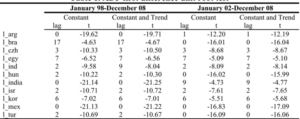
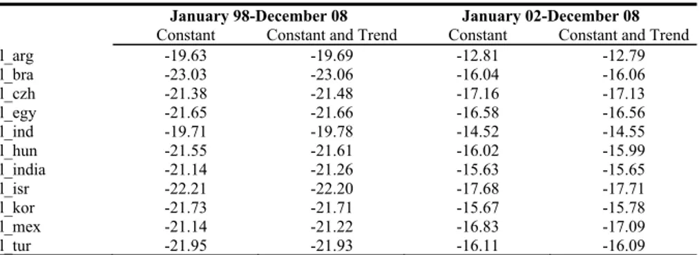
According to Enders (1995), long term equilibrium relations between the variables are defined as cointegration. For this reason, it is aimed to use Johansen multiple cointegration test to analyse the long term relation between these 11 countries. In the Johansen cointegration test, the time series should be in the same degree of stationarity. Therefore, unit root tests are applied to the difference of time series. As can be seen in Table 1, 2, and 3 all the series are stationary on the level of first differences for the Augmented Dickey Fuller, Phillips-Perron and Kwiatkowski-Phillips-Schmidt-Shin tests respectively. In this framework, it can be observed that when we use the first difference stationarity test results, Johansen cointegration method can be used for all countries.

Table 1. ADF first difference unit root test

January 98-December 08 January 02-December 08

Constant Constant and Trend Constant Constant and Trend lag t lag t lag t lag t

l_arg 0 -19.62 0 -19.71 1 -12.20 1 -12.19 l_bra 17 -4.63 17 -4.67 0 -16.01 0 -16.04 l_czh 3 -10.33 3 -10.50 3 -8.68 3 -8.67 l_egy 7 -6.52 7 -6.56 7 -5.09 7 -5.10 l_ind 2 -9.58 9 -8.04 2 -8.09 2 -8.14 l_hun 2 -10.22 2 -10.30 0 -16.02 0 -15.99 l_india 0 -21.14 0 -21.25 9 -4.73 9 -4.77 l_isr 2 -10.71 2 -10.72 2 -7.61 2 -7.65 l_kor 6 -7.02 6 -7.01 6 -5.51 6 -5.68 l_mex 0 -21.13 0 -21.22 0 -16.83 0 -17.09 l_tur 2 -10.69 2 -10.67 0 -16.09 0 -16.06

Table 2. PP First difference unit root test

January 98-December 08 January 02-December 08

Constant Constant and Trend Constant Constant and Trend

l_arg -19.63 -19.69 -12.81 -12.79 l_bra -23.03 -23.06 -16.04 -16.06 l_czh -21.38 -21.48 -17.16 -17.13 l_egy -21.65 -21.66 -16.58 -16.56 l_ind -19.71 -19.78 -14.52 -14.55 l_hun -21.55 -21.61 -16.02 -15.99 l_india -21.14 -21.26 -15.63 -15.65 l_isr -22.21 -22.20 -17.68 -17.71 l_kor -21.73 -21.71 -15.67 -15.78 l_mex -21.14 -21.22 -16.83 -17.09 l_tur -21.95 -21.93 -16.11 -16.09

Table 3. KPSS first difference unit root test

January 98-December 08 January 02-December 08

Constant Constant and Trend Constant Constant and Trend

l_arg 0.34 0.06 0.09 0.05 l_bra 0.15 0.04 0.16 0.11 l_czh 0.37 0.06 0.07 0.06 l_egy 0.23 0.09 0.15 0.13 l_ind 0.26 0.03 0.14 0.07 l_hun 0.23 0.05 0.11 0.10 l_india 0.35 0.06 0.15 0.09 l_isr 0.14 0.08 0.17 0.10 l_kor 0.06 0.05 0.31 0.11 l_mex 0.28 0.04 0.44 0.09 l_tur 0.06 0.05 0.06 0.05

Moreover, further analysis suggested that all of the series are neither [I(2)] nor [I(3)]. As stated above, all of the series are stationary [I(1)] at the difference level. As it has been known, cointegration test is very liable to number of lags. Due to this, it has been decided to use the information criteria as the number of lags. It can be seen in Table 4 that Akaike, Schwarz, Hannan-Quinn and Final Prediction Error (FPE) indicate that the optimum number of lags is 1.

Table 4. VAR lag number calculation criteria

Lag LogL FPE AIC SC HQ

0 2892.611 2.58E-20 -13.88728 -13.78051 -13.84506 1 9200.353 2.90e-33* -43.70291* -42.42162* -43.19624* 2 9297.362 3.26E-33 -43.58729 -41.13149 -42.61618 3 9386.723 3.81E-33 -43.43481 -39.80451 -41.99926 4 9464.966 4.71E-33 -43.22875 -38.42394 -41.32876 5 9548.324 5.69E-33 -43.04734 -37.06802 -40.68291 6 9650.92 6.31E-33 -42.95865 -35.80481 -40.12977 7 9761.333 6.76E-33 -42.90763 -34.57928 -39.61431 8 9854.296 7.93E-33 -42.77251 -33.26965 -39.01475

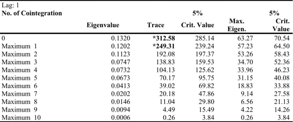
In the Johansen cointegration test (1990) the cointegration between the non-stationary series is identified according to the trace and maximum eigenvalue statistics. As indicated by the information criteria, the first lag of variables is also added to the VAR equation.

Table 5 shows the number of cointegration equations for the 5 % significance level. According to the trace statistic, there are 2 different cointegration equations which represent long-term relationship between the stock markets. On the other hand,

maximum eigenvalue statistic indicates that there is only one cointegrated relationship for the fourth and fifth models. For the remaining three models no cointegration equation can be found.

Table 5. Cointegration models and vector numbers

Series: L_TUR L_BRA L_ARG L_CZH L_EGY L_IND L_HUN L_INDIA L_ISR L_KOR L_MEX Lag Interval: 1 to 1

Number of cointegrated equations for the 5% significance level

(Data Trend) None None Linear Linear Parabolic

(Cointegration No Const. No Const. Constant Constant Constant

Vector) No Trend No Trend No Trend Trend Trend

Trace 2 2 2 2 2

Max-Eigenvalue 0 0 0 1 1

For the next step, out of Eviews models, the one, which has trend but not the constant in the equation and in which the returns are in linear order, has been chosen. The critical values, maximum and trace statistics have been shown in the table below as follows:

Table 6. Trace and Eigenvalue comparison test statistics Lag: 1

No. of Cointegration 5% 5%

Eigenvalue Trace Crit. Value _Eigen. Max. _Value Crit.

0 0.1320 *312.58 285.14 63.27 70.54 Maximum 1 0.1202 *249.31 239.24 57.23 64.50 Maximum 2  0.1123 192.08 197.37 53.26 58.43 Maximum 3  0.0747 138.83 159.53 34.70 52.36 Maximum 4  0.0732 104.13 125.62 33.96 46.23 Maximum 5  0.0673 70.17 95.75 31.15 40.08 Maximum 6  0.0413 39.02 69.82 18.83 33.88 Maximum 7  0.0202 20.18 47.86 9.14 27.58 Maximum 8  0.0146 11.04 29.80 6.56 21.13 Maximum 9  0.0094 4.49 15.49 4.22 14.26 Maximum 10 0.0006 0.26 3.84 0.26 3.84

* H0 rejected at the 5% significance level

As can be seen in Table 6, the result of the trace statistics shows that maximum 1 cointegration hypothesis has been rejected with 5% significance. On the other hand, the hypothesis which indicates maximum two cointegration equations has not been rejected with 5% significance. For this reason, it has been concluded that there are two cointegration equations that indicate long term relation. In a similar way, cointegration null hypothesis is not rejected with 5% significance using maximum eigenvalue critical values. As a result, according to maximum eigenvalue critical values, there is no long term relation between these 11 countries.

However, Johansen and Juselius (1990), Alexender (2001) and Onay (2006) state that the tendency should be towards the trace statistics if there is a difference between two statistics which analyze the number of cointegration vectors. For this reason, the research continues with the acceptance of two cointegration equations that are shown as a result of the trace statistics.

The equations for the cointegration are as follows:

L_TUR(-1) = - 4.95*L_ARG(-1) + 15.86*L_CZH(-1) + 1.48*L_EGY(-1) - 6.68*L_IND(-1) - 10.86*L_HUN(-1) + 4.05*L_INDIA(-1) - 1.17*L_ISR(-1)

- 2.49*L_KOR(-1) + 4.25*L_MEX(-1) + 23.63 + ut

(5) L_BRA(-1) = - 0.03*L_ARG(-1) + 0.15*L_CZH(-1) + 0.31*L_EGY(-1) -

0.55*L_IND(1) 0.52*L_HUN(1) + 0.51*L_INDIA(1) + 1.10*L_ISR(1) -0.42*L_KOR(-1) + 0.51*L_MEX(-1) + 2.27+ ub

(6) ut and ub are the error terms in N~(0,σ2).

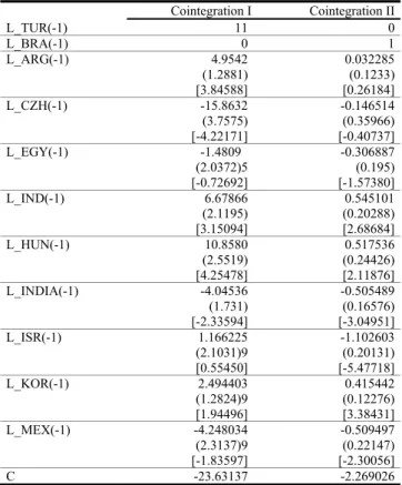
According to Table 7, in the first cointegration equation, the variables that belong to Egypt, Isreal, Korea and Mexico are not rejected with 5% significance. This tells us that the changes in those markets have no effect on Turkey. In a similar way, in the second cointegration equation, in which Brazil is the depedent variable, the variables that belong to Argentina, Czech Republic and Egypt are not rejected with 5% siginificance. Thus, the changes in those markets have no effect on Brazil. The variables of normalized cointegrating coefficients that are adapted for Turkey and Brazil within the Johansen test are shown in Table 7.

Table 7. Cointegration vector table

Cointegration I Cointegration II L_TUR(-1) 11 0 L_BRA(-1) 0 1 L_ARG(-1) 4.9542 0.032285 (1.2881) (0.1233) [3.84588] [0.26184] L_CZH(-1) -15.8632 -0.146514 (3.7575) (0.35966) [-4.22171] [-0.40737] L_EGY(-1) -1.48091 -0.306887 (2.0372)5 (0.195) [-0.72692] [-1.57380] L_IND(-1) 6.67866 0.545101 (2.1195) (0.20288) [3.15094] [2.68684] L_HUN(-1) 10.8580 0.517536 (2.5519) (0.24426) [4.25478] [2.11876] L_INDIA(-1) -4.04536 -0.505489 (1.731) (0.16576) [-2.33594] [-3.04951] L_ISR(-1) 1.166225 -1.102603 (2.1031)9 (0.20131) [0.55450] [-5.47718] L_KOR(-1) 2.494403 0.415442 (1.2824)9 (0.12276) [1.94496] [3.38431] L_MEX(-1) -4.248034 -0.509497 (2.3137)9 (0.22147) [-1.83597] [-2.30056] C -23.63137 -2.269026

In the long term, Czech and Indian markets affect Turkish stock markets. On the other hand, changes in Argentinian, Indonesian and Hungarian markets affect

Turkey in an inverse way. Second cointegration equation points out the fact that Brazilian stock market affects Mexican, Israeli and Indian stock markets in a parallel way, but Korean, Indonesian and Hungarian markets in an inverse way.

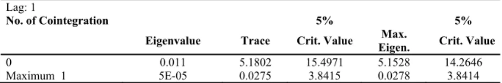
Here, results should be analyzed carefully. The reason for this is that in the cointegration equations long term variables are simultaneously structuralized. They point at a whole. For example, it would be wrong to assume that when Argentinian stock market increases, Turkish stock market drops down a level. This is just one of the possibilities. Despite they might have an inverse relation, they might both increase or drop. The best example is between years 1998 and 2008. According to the Figure 1, both markets increase at the same time. Although it seems as if the whole situation is contradictory, the reason for it is that the increase in parallel markets, such as Czech Republic and India, is much more than that of in the inverse markets such as Argentinian, Indonesian and Hungarian. Moreover, when we use the Johansen method to study the relation between the Argentinian and Turkish markets, in Table 8, it can be seen that both trace and maximum eigenvalue statistics show no cointegration between the two countries.

Table 8. Trace and maximum eigenvalue comparisons between

Argentina and Turkey

Lag: 1

No. of Cointegration  5% 5%

  Eigenvalue Trace Crit. Value _Eigen. Max. Crit. Value

0 0.011 5.1802 15.4971 5.1528 14.2646

Maximum 1 5E-05 0.0275 3.8415 0.0278 3.8414

Engle and Granger (1987) show that, if cointegration is detected between the variables, there is a vector error correction model. In this way, long term equilibrium and short term dynamics can be separated. In order to do this, we add error terms in the cointegration equation to the first difference of the variables. Cointegration equation shows the long term equilibrium. The excesses show the short term disequilibrum. As a result of this, the lost long term error term has been included in the model.

Error Correction parameter is used to hold the model dynamic in balance and compels the variables to be closer to long term equilibrium. The significance of the error correction parameter shows the deviation. Coefficient magnitude shows the rate of getting closer at the equilibrium. In practice, it is expected that the error correction parameter to be negative and statistically significant. In this situation, it is expressed that the variables will move toward the equilibrium number. The short term deviations are corrected according to the coefficient. The results of the Vectorial Error Correction are shown in Table 9. The error terms of the cointegration equation (CointEq1 and CointEq2) are added to the equation with one lag. The only country that the first cointegration equation is 5% significant is Argentina. However, although it is significant, the coefficient is as less as -0.007. This indicates that the correction process will be slow and gradual. The expectation that the Argentinian market will turn to its equilibrium is small due to its rejection of its coefficient to be different than zero. Markets which have 5% significance and whose error correction is negative are Brazilian and Czech markets. The Brazilian market has the coefficient of -0.09775 and this means that it will take approximately 10 weeks to turn back to its equilibrium.

Table 9. Vector Error Correction Model

Hata Düzeltme D(L_TUR) D(L_BRE) D(L_ARG) D(L_CEK) D(L_EGY) D(L_END) D(L_HUN) D(L_IND) D(L_ISR) D(L_KOR) D(L_MEX) CointEq1 -0.003846 0.00601 -0.006974 0.006944 -0.000129 -0.002256 0.002502 0.002624 -0.002343 -0.002888 0.000212 (0.00380) (0.00265) (0.00283) (0.00173) (0.00124) (0.00208) (0.00218) (0.00206) (0.00163) (0.00245) (0.00206) [-1.01220] [ 2.26829] [-2.46484] [ 4.00559] [-0.10374] [-1.08233] [ 1.14803] [ 1.27549] [-1.43772] [-1.17782] [ 0.10316] CointEq2 0.075525 -0.09775 0.04705 -0.038793 0.016593 0.015988 -0.022531 0.012895 0.045415 -0.005271 -0.011892 (0.03886) (0.02710) (0.02893) (0.01773) (0.01269) (0.02132) (0.02229) (0.02104) (0.01667) (0.02508) (0.02102) [ 1.94355] [-3.60763] [ 1.62612] [-2.18823] [ 1.30783] [ 0.75002] [-1.01102] [ 0.61299] [ 2.72495] [-0.21018] [-0.56569] D(L_TUR(-1)) -0.062116 -0.010546 0.041056 0.02304 0.016926 0.027085 0.016366 -0.023367 0.007819 0.056704 0.04598 (0.05298) (0.03694) (0.03945) (0.02417) (0.01730) (0.02907) (0.03039) (0.02868) (0.02272) (0.03419) (0.02866) [-1.17235] [-0.28546] [ 1.04068] [ 0.95316] [ 0.97841] [ 0.93186] [ 0.53861] [-0.81464] [ 0.34407] [ 1.65829] [ 1.60409] D(L_BRE(-1)) 0.1586 -0.154436 -0.154585 0.004352 0.008098 0.093831 -0.025463 0.06083 -0.056645 -0.020189 -0.018592 (0.09083) (0.06333) (0.06763) (0.04144) (0.02966) (0.04983) (0.05209) (0.04917) (0.03896) (0.05862) (0.04914) [ 1.74611] [-2.43848] [-2.28576] [ 0.10503] [ 0.27307] [ 1.88319] [-0.48884] [ 1.23709] [-1.45407] [-0.34441] [-0.37836] D(L_ARG(-1)) 0.157053 -0.055528 0.116277 0.019116 0.029815 -0.015614 0.032991 0.00389 0.071265 0.044882 0.028801 (0.07575) (0.05282) (0.05640) (0.03456) (0.02473) (0.04155) (0.04344) (0.04101) (0.03249) (0.04888) (0.04098) [ 2.07338] [-1.05135] [ 2.06166] [ 0.55316] [ 1.20555] [-0.37576] [ 0.75947] [ 0.09485] [ 2.19362] [ 0.91812] [ 0.70283] D(L_CEK(-1)) -0.181592 0.171474 -0.008353 0.038367 0.050716 -0.119449 0.134945 -0.025151 0.009877 -0.001184 -0.016448 (0.13141) (0.09163) (0.09785) (0.05995) (0.04291) (0.07209) (0.07536) (0.07114) (0.05636) (0.08481) (0.07109) [-1.38184] [ 1.87137] [-0.08537] [ 0.63996] [ 1.18201] [-1.65699] [ 1.79061] [-0.35353] [ 0.17524] [-0.01396] [-0.23136] D(L_EGY(-1)) -0.178822 -0.126773 -0.182341 -0.148479 -0.030562 -0.003252 -0.109188 -0.046388 -0.073674 -0.13072 -0.140731 (0.15351) (0.10703) (0.11430) (0.07003) (0.05012) (0.08421) (0.08803) (0.08310) (0.06584) (0.09907) (0.08305) [-1.16492] [-1.18441] [-1.59534] [-2.12018] [-0.60978] [-0.03862] [-1.24031] [-0.55820] [-1.11902] [-1.31951] [-1.69462] D(L_END(-1)) -0.060914 0.088833 -0.043687 -0.036158 -0.027499 0.017774 0.040851 0.014758 0.003357 0.002819 0.016039 (0.09319) (0.06498) (0.06939) (0.04251) (0.03043) (0.05112) (0.05344) (0.05045) (0.03997) (0.06014) (0.05042) [-0.65365] [ 1.36712] [-0.62962] [-0.85050] [-0.90379] [ 0.34769] [ 0.76439] [ 0.29253] [ 0.08399] [ 0.04688] [ 0.31813] D(L_HUN(-1)) 0.040823 0.050393 -0.048691 -0.046456 -0.01646 0.076141 -0.107947 -0.069695 -0.013913 0.02466 -0.099388 (0.11805) (0.08231) (0.08790) (0.05385) (0.03854) (0.06476) (0.06770) (0.06391) (0.05063) (0.07618) (0.06386) [ 0.34582] [ 0.61223] [-0.55397] [-0.86261] [-0.42706] [ 1.17581] [-1.59454] [-1.09058] [-0.27480] [ 0.32369] [-1.55626] D(L_IND(-1)) -0.005003 0.097392 0.058903 0.102818 0.019346 -0.102276 0.049255 -0.050902 0.038215 0.054148 0.120945 (0.09778) (0.06818) (0.07280) (0.04461) (0.03192) (0.05364) (0.05607) (0.05293) (0.04194) (0.06310) (0.05290) [-0.05117] [ 1.42854] [ 0.80910] [ 2.30501] [ 0.60600] [-1.90686] [ 0.87841] [-0.96164] [ 0.91130] [ 0.85812] [ 2.28647] D(L_ISR(-1)) 0.066739 0.005234 -0.03828 -0.111882 -0.015255 -0.033622 -0.016276 -0.025526 -0.033683 0.095266 -0.006924 (0.12975) (0.00818) (0.00933) (0.00350) (0.00179) (0.00507) (0.00554) (0.00493) (0.00310) (0.00701) (0.00493) [ 0.51437] [ 0.05786] [-0.39625] [-1.89012] [-0.36011] [-0.47239] [-0.21874] [-0.36340] [-0.60528] [ 1.13770] [-0.09865] D(L_KOR(-1)) -0.014259 -0.007543 0.051627 -0.023077 0.047526 0.193052 -0.029326 0.085545 0.013755 -0.038159 0.068221 (0.08825) (0.06154) (0.06571) (0.04026) (0.02881) (0.04841) (0.05061) (0.04778) (0.03785) (0.05696) (0.04775) [-0.16156] [-0.12257] [ 0.78566] [-0.57315] [ 1.64936] [ 3.98765] [-0.57943] [ 1.79049] [ 0.36340] [-0.66998] [ 1.42887] D(L_MEX(-1)) -0.050685 0.159866 0.188505 0.088669 0.001528 0.138131 0.092549 0.126015 -0.018713 0.000351 -0.004191 (0.12465) (0.08692) (0.09281) (0.05687) (0.04070) (0.06838) (0.07149) (0.06748) (0.05346) (0.08045) (0.06744) [-0.40661] [ 1.83931] [ 2.03102] [ 1.55919] [ 0.03755] [ 2.02007] [ 1.29466] [ 1.86737] [-0.35001] [ 0.00436] [-0.06215] C 0.006714 0.002698 0.002253 0.003123 0.003702 0.002211 0.001634 0.002229 0.003149 0.00226 0.003819 (0.00321) (0.00224) (0.00239) (0.00146) (0.00105) (0.00176) (0.00184) (0.00174) (0.00138) (0.00207) (0.00173) [ 2.09357] [ 1.20667] [ 0.94358] [ 2.13458] [ 3.53594] [ 1.25696] [ 0.88832] [ 1.28383] [ 2.28946] [ 1.09217] [ 2.20145] R-squared 0.045225 0.07938 0.053286 0.072888 0.044794 0.124674 0.028098 0.051121 0.038611 0.030409 0.036071 Adj. R-squared 0.01656 0.05174 0.024862 0.045053 0.016115 0.098395 -0.001082 0.022633 0.009747 0.001299 0.007131 Sum sq. resids 1.905127 0.926237 1.056175 0.396513 0.203089 0.573282 0.626551 0.558342 0.350443 0.793477 0.557583 S.E. equation 0.066331 0.046251 0.049388 0.030261 0.021657 0.036387 0.038039 0.035909 0.028449 0.042808 0.035885 F-statistic 1.577699 2.871929 1.874714 2.618593 1.561936 4.744086 0.962933 1.794463 1.337699 1.044632 1.246402 Log likelihood 585.5998 746.782 717.4411 936.4044 1085.94 854.0066 834.1483 859.9086 964.0086 781.3587 860.2126 Akaike AIC -2.557493 -3.278667 -3.147387 -4.127089 -4.796153 -3.758419 -3.669568 -3.784826 -4.250598 -3.433372 -3.786186 Schwarz SC -2.429002 -3.150175 -3.018896 -3.998597 -4.667661 -3.629927 -3.541076 -3.656334 -4.122106 -3.304881 -3.657695 Mean dependent 0.005849 0.00322 0.002184 0.002917 0.003932 0.003062 0.001956 0.002401 0.00287 0.002487 0.003791 S.D. dependent 0.066887 0.047496 0.050014 0.030967 0.021834 0.038321 0.038019 0.036323 0.028589 0.042836 0.036013

As can be seen in Table 9, Czech market has the error correction coefficiency of -0.038793 and equilibrium time process should be 21-22 weeks. Moreover, both two countries have the first equation error correction coefficiency of, respectively, 0.00601 and 0.00694 and they both have the 5% significance difference. The positive coefficients show the break from the equilibrium. For the other stock markets, at the 5% significance level it can not be rejected that the error correction coefficients are other than zero. If the coefficient would be zero, the error correction model won’t response, and if it would be positive, the disequilibrium would grow more. Therefore, it can be said that for these countries the equilibrium is not permanent.

7. Conclusion and General Evaluation

This paper attempts to show the model of cointegration among emerging markets. It aims to shed light on future studies on emerging markets with different time series data. Our main contribution on the subject is the application of the cointegration model, interpretation of the results and the explanation of the relationship between emerging markets. In order to get these contributions, three separate unit root tests are applied in the study. Moreover, in order to detect the lag numbers, different tests are made due to the difference in the lag numbers provided by Akaike and Schwarz. All the tests between 1998 and 2008, point to the fact that, the index movements are random. Accordingly, it is examined whether or not it is possible to forecast the index of a market by analyzing the other if they are cointegrated. For this, at first, unit root tests are done for the first differences. All tests indicate that unit root asset is rejected in ADF and PP tests with the significance of 5%. In KPSS test, on the other hand, the first differences’ stationarity have not been rejected with the significance level of 5%. This made it possible to include all the countries in the Johansen cointegration test for the years between 1998 and 2008. Then, Johansen cointegration test is carried to 11 emerging markets with [I(1)] degree of stationarity. According to the cointegration model there are 2 different cointegration equations which represent long-term relationship between the stock markets. Due to the first cointegraiton equaiton, it can be said that in the long term, Czech and Indian markets affect Turkish stock markets. On the other hand, changes in Argentinian, Indonesian and Hungarian markets affect Turkey in an inverse way. Furthermore, second cointegration equation points out the fact that Brazilian stock market affects Mexican, Israeli and Indian stock markets in a parallel way, but Korean, Indonesian and Hungarian markets in an inverse way. In addition to this, a Vector Error Correction model is used in order to hold the model dynamic in balance. In the vector error correction model, there is no relation to correct the short term deviation of gaining returns above the normal level with 5% significance in the cointegration equation except in the Argentinian, Brazilian and Czech markets. This is considered to be parallel with the market efficiency. According to this model, the only country the first cointegration equation is 5% significant is Argentina in which the correction process will be slow and gradual. Moreover, markets which have 5% significance and whose error correction coefficient is negative are Brazilian and Czech markets. For the Brazilian market, it will take approximately 10 weeks to turn back to its equilibrium whereas the equilibrium process will take approximately 21-22 weeks for the Czech market.

Efficient Market Hypothesis covers a wide range of area from simple past prices to difficult insider trading. There are three assignments which claim that developed markets operate efficiently. Firstly, new information can be applied efficiently in the markets. Secondly, it is difficult to forecast the course of the public information in the coming time. Thirdly, even if the miscalculated prices exist, it is not possible to determine them with simple method which is based on public information. The main idea behind the hypothesis is that all information is ready to be applied. Thus, any kind of profit or return that is above the normal are contradictory to EMH. However, in developed markets, despite the existence of the anomalies, it is not proved that profits or returns can be above the normal due to the inefficiency of the markets. Moreover, even if there is a possibility of arbitrage in the developed markets, it is lost due to the investors’ ambition to use it. It is not possible to use financial resources in a productive way if the market does not operate efficiently. When we consider the underfund problem in most countries, market efficiency becomes much

more important. Harvey (1993) suggests investments in emerging markets due to their lack of informative efficiency. Actually, there were some studies in these countries to overcome the problem of underfunds. However, it is assumed that with the latest developments in technology, communication and economy, there is some improvement. With this thought, there has been a research that includes the stock indices of the 11 countries between 1998 and 2008.

The empirical studies show that there are enough anomalies in the market and it is not useless to detect the assets that are undervalued. However, most results emphasize the need to be careful about the winner strategy offer. The competition in markets enables only a very good put-call strategy to gain profits. To sum up, markets are highly efficient, but only careful, attentive and creative investors win. The increase in the interest in the emerging markets makes it more attractive for the institutional investors. Kelly (2005) in his study on New York market, points out to a parallel relation between company owner ratio and market efficiency.

On the other hand, the increase in cointegration may lead to some problems in the future. The difference between the countries disappear which at the same time, might lead to an increase in the problems concerning the diversification in the portfolio management. Increase in cointegration makes it meaningless to invest in different countries except in terms of liquidity. For this reason, sectoral distribution is important for diversification. Moreover, cointegration of so many countries makes it possible to think that the crisis in one country can lead to another one in the cointegrated countries. In order to avoid this, political structuralists should not interpret the relation as an increase in information and come up with measures.

8. References

ALEXANDER, C. (2001). Market Models: a guide to financial data analysis. 1st ed., Chichester: John Wiley & Sons Ltd.

BALABAN, E. (1995). Einstein, risk ve gümrük birliği. Ankara Üniversitesi Siyasal Bilgiler

Fakültesi Dergisi, 50 (1-2), 77-93. ss.

BERUMENT, H., İNCE, O. (2005). Effect of S&P 500 return on emerging markets: Turkish experience. Applied Financial Economics Letters, 1 (1), 59-64. ss.

BUGUK, C., BRORSEN, W.B. (2003). Testing weak-form market efficiency: evidence from the Istanbul Stock Exchange. International Review of Financial Analysis. 12 (5), 579-590. ss.

CERNY, A. (2004). Stock market integration and the speed of information transmission. research report 242. Prague: The Center for Economic Research and Graduate Education – Economic Institute.

CHEUNG, Y.L., MAK, S.C. (1992). A Study of the international transmission of stock market fluctuation between the developed markets and the Asian-Pacific markets. Journal

of Applied Economics, 2 (1), 43-47. ss.

CORHAY, A., RAD, A.T., URBAIN, J.P. (1993). Common stochastic trends in European stock markets. Economics Letters, 42 (4), 385-390. ss.

CROCI, M. (2003). An Empirical analysis of international equity market co-movements:

implications for informational efficiency. Research report 197. Ancona: Universita

Politecnica delle Marche.

DARRAT, A.F., ZHONG, M. (2000). On testing the random-walk hypothesis: a model comparison approach. The Financial Review, 35 (3), 105–124. ss.

DARRAT, A.F., BENKATO, O.M. (2003). Interdependence and volatility spillovers under market liberalization: the case of Istanbul Stock Exchange. Journal of Business Finance

EFENDİOĞLU, E., YÖRÜK, D. (2005). Avrupa Birliği sürecinde Türk hisse senedi piyasası

ile Avrupa Birliği hisse senedi piyasalarının bütünleşmesi: İMKB Örneği. Unpublished

Working Paper.

ENDERS, W. (1995). Applied dynamic econometrics. 1st ed., New Jersey: John Wiley. ENGLE, R.F., GRANGER, C.W.J. (1987). Cointegration and error correction:

pepresentation, estimation and testing. Econometrica, 55 (2), 251-276. ss.

ERDAL, F., GÜNDÜZ, L. (2001). An Empirical investigation of the interdepence of Istanbul Stock Exchange with selected stock markets. Global Business and Technology

Association International Conference, Istanbul.

EUN, C.S., SHIM, S. (1989). International transmission of stock market movements. Journal

of Financial and Quantitative Analysis, 24 (2), 241-256. ss.

FAMA, E. (1991). Efficient capital markets: II. Journal of Finance, 46 (5), 1575-1617. ss. GRANGER, C.W.J. (1986). Developments in the study of cointegrated economic variables.

Oxford Bulletin of Economics and Statistics, 48 (3), 213-228. ss.

HARVEY, C.R. (1993). Predictable risk and returns in emerging markets. Research report 4621. Cambridge: National Bureau of Economic Research.

JOHANSEN, S. (1988). Statistical analysis of cointegration vectors. Journal of Economic

Dynamics and Control, 12 (2-3), 231-254. ss.

JOHANSEN, S., JUSELIUS, K. (1990). Maximum likelihood estimation and inference on cointegration with application to the demand for money. Oxford Bulletin of Economics

and Statistics, 52 (2), 169–210. ss.

KANAS, A. (1998). Linkages between the US and European equity markets: further evidence from cointegration tests. Journal of Applied Financial Economics, 8 (6), 607-614. ss. KASA, K. (1992). Common stochastic trends in international stock markets. Journal of

Monetary Economics, 29 (1), 95-124. ss.

KELLY, P.J. (2005). Information efficiency and firm-specific return variation. Unpublished PhD Thesis, Arizona State University.

LEE, H.S. (2004). International transmission of stock market movements: a wavelet analysis.

Applied Economics Letters, 11 (3), 197–201. ss.

LENCE, S., FALK, B. (2005). Cointegration, market integration and market efficiency,

Journal of International Money and Finance, 24 (6), 873-890. ss.

LONGIN, E., SOLNIK, B. (1995). Is the correlation in international equity returns constant: 1960-1990? Journal of International Money and Finance, 14 (1), 3-26. ss.

MALATYALI, N.K. (1998). Seçilmiş borsa endeks getirileri arasındaki koentegrasyon ilişkileri üzerine bir araştırma. İMKB Dergisi, 2 (7-8), 23-34. ss.

MATHUR, I., SUBRAHMANYAM, V. (1990). Interdependencies among the Nordic and US stock markets. Scandinavian Journal of Economics, 92 (5), 587–597. ss.

ONAY, C. (2006). A Co-integration analysis approach to european union integration: the

case of acceding and candidate countries. Research report 10. European Integration

Online Papers.

ROLL, R. (1992). A Mean/variance analysis of tracking error. Journal of Portfolio

Management, 18 (4), 13-22. ss.

STOCK, J.H., WATSON, M.W. (1988). Variable trends in economic time series. Journal of

Economic Perspectives, 2 (3), 147-174. ss.

SWEENEY, J. (2003). Cointegration and market efficiency. Journal of Emerging Market

Finance, 2 (1), 41-56. ss.

VALADKHANI, A., CHANCHARAT, S., HARVIE, C. (2006). The Interplay between the

Thai and several other international stock markets. Research report 06-18. New South

Wales: University of Wollongong.

VORONKOVA, S. (2004). Equity market integration in Central Europe Emerging Markets: a cointegration analysis with shifting regimes. International Review of Financial Analysis, 13 (5), 633-647. ss.