A network model for rigid-body motion

(1)

A Network Model for Rigid-Body Motion

YILMAZ TOKAD

Department of Mathematics, Bilkent University, 06533 Bilkent, Ankara, Turkey Received September 11, 1990; revised February 26 and June 26, 1991 Editor: E.P Ryan

Abstract. In the formulation of equations of motion of three-dimensional mechanical systems, the techniques utilized and developed to analyze the electrical networks based on linear graph theory can conveniently be used. The success of this approach, however, relies on the availability of a complete and adequate mathematical model of the rigid body valid in the three-dimensional motion. This article is devoted to the derivation of such a mathematical model for the rigid body as a (k + 1)-port component. In this derivation, the dynamic properties of the rigid body are automatically included as a consequence of the analytical procedures used in the article. In this model, a general form of the terminal equations is given. In many applications, however, its special form, also given in this article, is used.

1. Introduction

In the formulation o f system equations or o f the equations of motion o f three-dimensional mechanical systems that contain rigid bodies, the establishment of a complete and compact mathematical model for the rigid bodies plays an important role. In the past three decades, formulation techniques developed and used in the study of electrical networks, based on linear graph theory, have also been conveniently applied to one-dimensional and to some restricted classes of higher-dimensional mechanical systems [1-5]. Recently, based on the same approach, these techniques have been extended to three-dimensional systems [6]. Since the crucial point in such a formulation procedure lies mainly in a thorough representation of rigid bodies, this article is devoted to the derivation of a general and compact mathematical model of a multiterminal rigid body valid in three-dimensional motion.

The mathematical model o f a component in a given system is formed by: 1) an oriented terminal graph, identifying the terminal pairs (ports) of the component and the orienta- tions of the associated instruments, real or conceptual, connected at the ports to measure a pair of complementary variables (one across and one through) to describe the physical behavior of that component, and 2) the terminal equations, giving the relationships be- tween all the measured across and through variables of the ports [2, 4]. These relations are also known as constitutive equations of the component. A terminal graph, being a col- lection of oriented edges, may or may not be connected; however, it does not contain any circuit, i.e., it is simply a tree or a collection of tress [7]. In three-dimensional motion, since the terminal variables are necessarily vectorial quantities, the terminal graphs to be used for the mechanical components can properly be named vector terminal graphs, with the understanding that these are equivalent, in the most general case, to six usual (scalar) component terminal graphs all having exactly the same topological form as the vector terminal graph. Each of the scalar terminal graphs is associated with the x-, y-, z- components

(2)

60 Y. T O K A D

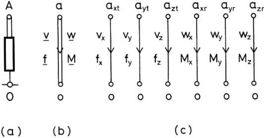
of either the translational or the rotational terminal variables at the ports. In the translational motion, the terminal variables are the linear velocity and the force, while in a rotational motion, these variables are the angular velocity and torque (torsional moment). In this article, in order to distinguish a vector terminal graph from a scalar one, the graph edges of the former are indicated by double lines. Because of this condensed representation of a terminal graph, a simple two-terminal (one-port) mechanical element in three- dimensional motion (see Figure la), such as an elastic beam with one terminal rigidly attached to a reference, will have a simple representation (see Figure lb), compared to its equivalent scalar representation if the terminal variables are resolved into their components (Figure lc). The choice of the terminal across through variables as velocities and forces (torques) for the mechanical components, as introduced by Firestone and Trent [1, 2], is useful in establishing the state equations of a given mechanical system. This choice is also consistent with the property that the product of two complementary terminal variables represents mechanical power. This property makes it possible to define such important components as

perfect couplers

or instantaneously powerless (nonenergic) multiterminal components [8-10]. Here, in the derivation of the mathematical model of a rigid body, these components are referred to as

ideal components.

On the other hand, in the formulation of the equations of an electrical network containing nonlinear elements, it may become necessary to consider the integral of either or both of the across and through variables. Since in three-dimensional motion the displacement relations are inherently nonlinear, in the final set of state equations of motion at least one or both of the integrated variables-- displacement and momentum (linear or angular)--will appear. In the classical Lagrange equations, however, momentum variables are eliminated through the formulation procedure, yielding the equations of motion in the form of a set of second-order differential equations in the displacement (generalized coordinates) variables [11].

A

a

V

W

f

M

m m

0 o

O.xt

?

0 Qyt

Qzt

O'xr Qyr

O'zr

0 0 0 o 0

Vy

Vz

Wx

wy

w7

i xl/ xv '~/ W

fy

fz

Mx My Mz

0 0 0 0

0

0 (a)

(b)

(c)

Figure 1. (a) A two-terminal (one-port) component with terminals A and O (reference). Co) The vector terminal graph with the vertices a and o corresponding to the terminals A and O of the one-port component. (c) The scalar terminal graph as the components of the vector terminal graph in Figure lb.

(3)

A NETWORK MODEL FOR RIGID-BODY MOTION 61

2. Mathematical model of a rigid body

One of the approaches to developing a mathematical model of a given complicated component included in a system is to decrease its complex appearance by decomposing it, at least conceptually, into some lumped simple elements so that the component is reduced into its simplest possible form. However, the simple form so obtained should preserve the essen- tial properties of the original component. This reduction process may properly be called an idealization of the original component [14]. The idealized component may be hypothetical, but its terminal equations are assumed to be algebraic. This point of view is actually the basic idea used in network synthesis, where the idealized components turn out to be perfect couplers that are either the multiterminal ideal transformer or the gyrator in the passive case and dependent drivers (sources) in the active case [15, 16]. Since this decomposition is not unique, different types of such representations for the same component are possible. Representing complex components as the collection of ideal multiterminal algebraic components together with simple, usually two-terminal elements provides us with a systematic procedure to obtain the state equations of a given system [17]. Since our aim here is to establish a mathematical model for the rigid bodies, we have a rather simple case to consider for modeling; i.e., only two types of components are involved. Indeed, a rigid body (61) with a known mass distribution can be considered as a massless solid geometrical figure (610) loaded at some of its B i terminals by discrete (point) masses, each having usually a different mass value. It is plausible that the number of these discrete masses can be increased at will to improve the representation so that it is more valid for the body. On the other hand, it is known that to use at most six such discrete mass elements will be sufficient to create an equimomental rigid body [19]. However, this property should directly follow after the establishment of a general mathematical model for the rigid body. As will be see in the following discussion, the network analog to the ideal rigid body (610) is a multiport ideal transformer. Since only the port voltages v(t) (across variables) and also only the port currents i(t) (through variables) are interrelated, for a multiport ideal transformer the terminal equations of a p-port ideal transformer will necessarily be in the following form:

Av(t) = : ) Bi(t)

(1)

Assume that rank (A) = Pl < P. Then partitioning v(t), the first relation in equation (1) can be put into the form

(Pl) Vl(I) = Nv2(t) (2)

Since, from the definition of ideal transformer, its instantaneous power

Iill

13(t ) = vTi m- [V T V T] = vTil "~ vTi2 ~ 0 i2

(4)

62 v. TOKAD

is identically equal to zero for all values of the terminal variables, substitution of equation (2) into equation (3) gives

i,(t) = v2rNril + v~i2 = v2 r (Nril + i2) - 0,

(4)

which yields

(P - Pl = P2) i2 = - Nril. (5)

This is actually the second relation in equation (1), and therefore a more detailed form of the terminal equations of ap-port ideal transformer is seen to be in the following form:

i o .]

i,,t>l

(P2) i2(t) - N T O v2(t )

(6)

Note that the coefficient matrix in equation (6) is skew symmetric. Due to the zero submatrices in the terminal equations, neither all v nor all i can be expressed in terms of the remaining terminal variables. Therefore, on both sides of equations (6), there will always be a mixture of voltage and current variables. For this reason, the terminal euations (6) are called hybrid or mixed.

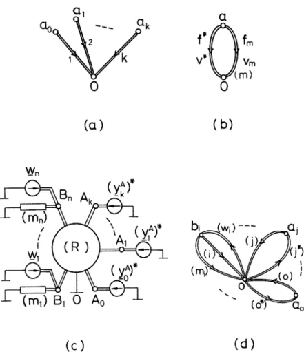
Let the Bi (i = 1, 2 . . . n) represent points where the discrete masses of known values are attached, and let the Aj (j = O, 1 . . . . , k ) represent the terminal points of interest on the solid geometrical figure (610), which hereafter will be called a massless or ideal rigid body. Therefore, including the inertial reference O, the ideal rigid body (610) is considered as an (n + k + 1)-port component with the B i, Aj, and O as its terminals, while the original rigid body (61) is considered as (k + 1)-port component having only the terminals

Aj and O, as indicated in Figure 2(a). It is asumed that a sufficient number of B i points on (610) were chosen, each being associated with an appropriate mass value mi, such that two of the necessary conditions for the equivalence of discrete representation and the rigid body itself are satisfied, i.e. 1) r. n , i=1 mi is equal to the mass m of the rigid body (61), and

2) the center of mass of n point masses coincides with that of the rigid body (61). The complete condition, both necessary and sufficient for the equivalence, includes also the requirement that the rigid body and its corresponding discrete representation must possess identical mass moment-of-inertia matrices with respect to the same (otherwise arbitrary) reference system. Actually, equivalence considerations can be deferred until the establishment of the mathematical model of the rigid body, since in the following discussion we only need to use a finite set of point masses.

(5)

( R

o)

Bi

B~

A}

bn ~ak

B I -

Ak

B?

.L. 0

o

(a)

(b)

(c)

Figure 2. (a) An ideal (n + k + D-port rigid body ((~) with terminals Bi's , Aj's, and O. (b) The terminal graph. (c) A pictorial representation of (6[).

2.1. Mathematical model of an ideal rigid body

To establish the terminal equations of a multiterminal ideal rigid body ((Ro) (see Figure 2a), consider its terminal graph given in Figure 2b. In order to distinguish the terminals of the component from the corresponding vertices of its terminal graph, vertices are labeled by lower-case letters [5]. A few preliminary remarks are in order:

Remark 1. Since the body is rigid, its kinematics is completely determined in terms of the across variables (the displacements or velocities) at only one of its ports. More specific- ally, this port is selected as (A0, O) with the across variables ~ ( t ) and <o~(t). Remark 2. Since the rigid body is ideal, the instantaneous power (sum of the instantaneous powers at the ports) is identically equal to zero. Hence, considering also remark 1, the terminal equations (being necessarily algebraic) can only be written in the hybrid (mixed) form with a skew-symmetric coefficient matrix, analogous to equations (6).

Remark 2 implies, in turn, that the terminal through variables, i.e., forces and moments at the ports, are also interrelated. This relation is known as the equation of equilibrium (statics) of the ideal rigid body and can be written directly as a consequence of the kinematic information, rather than by considering a free-body diagram of the ideal rigid body. The converse of this statement is also true. In the following, we shall consider first the equations of equilibrium. Let the terminal variables at the ports (Bi, O) and (Aj, O) (i = 1,

(6)

6 4 Y. T O K A D (6) (6)

x~(t)

yfl(t)

- v~(t)

o~(t)

I 1

I

fr(t)

I

_ M f ( o J

xA(t) Y~(/)

-

vJ(t)

,¢(t)

I

rf~(0

_

_1

(7)

where, e.g., v/B, c0f represent third-order column matrices corresonding to the linear and angular velocities, respectively (across variables), while ffl, M~ represent third-order column matrices corresponding to the force and the moment (torque), respectively (through variables), at the port

OBi.

Note that the column matrices x i and Yi are also called the

twist

and the

wrench,

respectively. Then the well-known equations of equilibrium,

f ~ = O a n d ~ M i + ~ (~ ×fT) = O,

can be written more explicitly, as the following matrix form:

Eo...o,o...o

1

(3) I . . . I I I ' " I

M1B(t)

M~(t)

MA(t)

= [

I'"I I I'"I ]

Rf R ~ I I ~ R~ -

if(t) 1

fn"(') I

foA(t)

_ f~(t) J

= 0 ,

(8)

where I denotes the 3 × 3 unit (identity) matrix, 0 is a 3 × 3 zero matrix, and R/B and R~ are 3 × 3 skew-symmetric matrices corresponding to the position vectors r/B and rj A of the points

Bi and Aj,

respectively, relative to O. All the quantities are expressed in a right-hand rectangular Cartesian coordinate system S, which is assumed to be inertial. Representation of vectors by column or skew-symmetric matrices is useful, and their further properties are presented in the appendix [12, 13]. By simple manipulations, the relation in equation (8) can be put into the following form:

(7)

A NETWORK MODEL FOR RIGID-BODY MOTION

65 (3)[ f64(t) I =

(3)

Mff(t)

- f~(t) 1

I

• 1 : l

I

I I

fff(t) ]

I - I

0 I

I

-s8x - I J

I - I 0 I - I 0 [ I - I 0 7 I I I . . . I

]

I-ago - I U - l ~ - I I

) - S ~ - I

MnB(t)

fi4(t)

Mr(t)

(9)

,I

f~(t)

where the new third-order skew-symmetric matrices, defined as

R~/ = R~ - R~, R~ = R~ - R~,

(10)

represent, respectively, the position vectors roB/and r~j of the points

B i

and

Aj,

relative

to A0 in S. With a more compact matrix notation, equations (9) can be expressed as in

the following form:

(8)

66 Y. TOKAD

- ~ ( t ) -

v~(t)

(6) y~(t) = [ - K f . . . - K B I - K ( . . . - K A] m__ ~ ( t )

~(t)

(11)

with

[ f~(t) ]

[ fF(,) ]

L~(t)J

LMf(,)J

[to I [,o 1

, K~

K~

Ro",. I

a~ I

[ f?(') ]

M;(t)J

*,

(12)

(i = 1, 2 . . . . , n; j = 1, 2 . . . k). This relation constitutes the portion of the terminal euqations of the ideal rigid body (610) given pictorially in Figure 2c. To obtain a complete expression for the terminal equations, kinematic relations that exist between the terminal across variables x~/(t) and xflj (t) must be considered. However, these relations will follow immediately from equation (1 1) due to remark 2 above, and hence the complete terminal equations containing both the equilibrium and kinematic equations of the ideal (n + k + 1)- port rigid body (610) will necessarily have the following hybrid form:

(6n)

(6k)

(6)

- xf(t) "

~ ( t )

~ ( t )

y~0 (t)

- K ~ . . . - - K B j - K ( . . . --KAI I (K1B) T-

(Ky) r

(Kf) r

(KD r

- ~ ( t )

ynB(t)

~ ( t )

if(t)

_x~(t)_

, (13)

(9)

A N E T W O R K M O D E L F O R RIGID-BODY M O T I O N 67

where all the entries in the empty spaces are zero and are therefore not shown explicitly. It will be instructive to look closely at the kinematic portion of the terminal equations in (13). For instance, at the port

(Bi, O)

we have the relation x/S(t) = (Kfl) r ~ ( t ) , which may be written explictly as

El 1 1

coiB(t)

0

I

COoa(t)

(14)

where the second row-block, ¢0/~ = ¢0o a, states that the angular velocities at the ports of the ideal rigid body are identical. However, from the first row-block, we have

J

(15)

where the property 2 in table A1 of the appendix is used. Note that the 3 x 3 skew-symmetric matrix fl~ represents the angular velocity o~oo of the rigid body. Also note that the kinematic portion of equations (13) is peculiar to the rigidity of the rigid body and is valid whether assumed to be ideal or not.

2.2. The inertia matrix

Consider a rigid body (61) fixed with respect to a Cartesian coordinate system S. Let B be a point on (61) with the position vector r = [Xl,X2,

x3] r

expressed in S, and let the mass of the infinitesimal volume

dV

of (61) in the neighborhood of B be

dm.

By definition, the inertia matrix J0 of (61) with respect to S has the form [11, 19]

-h2 62

-63 -123

Jo = where

h~ -62 -h3

63 I l l =

fv(4 + 4) dm,

I22 =

fv(~ + ~) am,

133 =

fv(~ + 4) dm ~ ,

J

112

fv XlX2dm,

113 =

fv

XlX3 dm,

123 =

fv x2x3dm

(16)

and

(10)

68 Y. TOKAD

I0 =_1 trJo =_1 (IH + 122 +133) = f r r rdm

2 2 v (17)

represents the moment of inertia with respect to the origin. Since one can write

[

4 + ~ -xlx2 -x:3]

- x : 2 x~ + ~

-x2x3 [ =

I -XlX3 - x : 3 + 4_1 0 - x 3 x2 ]

l

x3 0 - x l - x 2 xl 0

o x3 1

- - X 2 - - X 3 0 = R R T, x2 - x l (19)

Jo may be put in the following lbrm:

J0 = ( R R r dm. (19)

d V

Although the third-order skew-symmetric matrix R is singular, and hence RR r is positive semidefinite, the integral in equation (19) generally produces a positive-definite symmetric matrix. On the other hand, the mass of (6t) is m = fv din, and the point G defined by

if

roG - rdm or Ro6 = N Rdm (20)

m v m v

is called the center of mass of (6t). When ( ~ ) is considered as a collection of n discrete masses located at the points Bi, which are obtained through a discretization process of ( ~ ) , then the expressions in equations (17), (19), and (20) can be replaced, respectively, by the following expressions:

n B T B

Io = ~i=1 mi(roi) (roi)

)

Jo ₌~;?=1 _{miRoi(Roi )}B B T _•

mRoG = ~,n miR~i i = 1

(21)

In other words, the integrals are placed by the sum of a finite number of terms. If only the translation of coordinate axes S to the center of mass G of ((R) is of interest, we have

~_. n B B T

Jo = J c + mRoGR~G (Ja ~i=1 miRGi(RGi) ), (22) where J~ is the mass moment of inertia matrix of ((R) with respect to G, the 3 × 3 skew symmetric matrix R~i indicates the position vector of B; with respect to the translated coordinate system, and ROG is given as in equation (20). This property is known as the parallel axes theorem [19]. Since J 6 is also symmetric and positive definite, it can be brought into a diagonal form by an orthogonal transformation [18]. This can be accomplished simply by rotating the translated coordinate system around its origin G so that it coincides with

(11)

the principal axes of the inertia ellipsoid of (fit) at G. Because of this property, the rigid body (fit) can be represented by an equivalent system having at most three pairs of discrete masses such that each pair is located symmetrically on each principal axis through G with proper distances from G, having a diagonal inertia matrix identical to that of (fit) (equimomental system) [19].

2.3. A general model for the rigid body

It must be expected now that, if the rigid body (fit) is not ideal--i.e., having a continuous or discretized mass distribution--its terminal equations corresponding to the terminal graph in Figure 3a will again be in a form similar to that in equations (13), except for the square submatrix in the far right of the last row-block, which is now a nonzero matrix. To derive these equations, (fit) is considered as an (n + k + 1)-port ideal rigid body (fit0) together with n discrete (point) masses mi attached at its points B~. Since the terminal equations of simple one-port discrete mass components are of the form [5] (Newton's Law),

d

(3) fi(t) = mi - -

vi(t)

(i = 1, 2, . . . , n) (23)

dt

no terminal moments at the ports (B i, O) exist. Therefore, in equations (13) we may as well use this information. Discarding the obvious restrictions ¢0/n(t) =¢Oo A (t) on the angular velocities and M~/(t) = 0 at the ports, the equivalent terminal equations of the (n + k + 1)- port ideal rigid body (fit0) now become

(3n) - VS(t) 1

/

(6k) xA(t)

(6) Y~0 (t)

F

I

t _ K s - K A

I(KS) T"

I

I ( K A ) T

1 ~_______

I

- fs (t) ] Y~(t) l

x~(t)_]

(24)

where the column matrices v B and fB represent the terminal linear velocities and forces, respectively, at the ports (OBi), while x A and ya stand for the terminal linear and angular velocities and also all terminal forces and torques, respectively. The submatrices in (Ka)r are in the same form of that in equations (12), while the submatrix K B now takes on a simpler form:

I

. . .

I ]

K B

=

Ro B, R~2 . , . Ronn

(12)

70 Y, TOKAD

0

(1

v t\ //Vm

V C m )

0 ( a )

(b)

~-n

_L '(~j \

//,',--,'-

" ;, ~

,,. (,

A),

_wl

a

' { ~ , D-

;T ¢/-2

b ~ = ~ ) - - -

~ a j

( m i ) ~ o

)

;

...o~-~

-

(o,~:~:=~o

(c)

(d)

Figure 3. (a) The terminal graph of a (k + 1)-port rigid body. (b) Graph of a point mass excited with a force

driver f*, (c) A schematic diagram of the rigid body represented as the interconnection of an (n + k + 1)-port ideal rigid body (61) and one-port mass components together with the gravity forces. (d) The system graph corresponding to the system in Figure 3c.

(13)

Since the terminal equations given in (23) for one-port mass components are valid only in an inertial reference system, the chosen rectangular coordinate system S is assumed to be inertial. Equations (23) can be written in the matrix form

, 4

(3n) fro(t) = Md ~ Vm(t), (26)

dt

where Md is a diagonal matrix partitioned into 3 × 3 blocks mlI, m21 . . . . , toni. Note that in both equations (23) and (26), for force variables f/and fm are the terminal forces. They may be regarded as the reaction forces. Indeed, if a mass component m is excited by an external force f*, then it follows from the simple graph in Figure 3b that

d f* = --fro = --m - - V m.

dt

Note that the relation f* + f m = 0, or, in general, the cut-set equation ~i fi = 0 is called D~dembert's principle.

In order to derive the desired terminal equations corresponding to the terminal graph in Figure 3a, the rigid body (6/) will be excited by the through drivers (y])* at its ports

(Aj, O). All of these connections are indicated on a schematic diagram in Figure 3c, where the force sources wi = mig due to gravity are also included. The acceleration of gravity g measured in the inertial system S is assumed to have the form

g =

0 0 - g

, (g = 9.81m/s2). (27)

Therefore, the complete system graph [5] indicating the interconnection pattern of the components will be as shown in Figure 3d, from which the independent set of circuit and cut- set equations can be written. Since at the final stage of the formulation procedure, the through (y])* and the across (x~j)* variables of the drivers must be expressed in terms of the terminal variables (yj4) and (x~j), respectively, and since

=

J

4=(4;

(28)

we may as well use the terminal variables instead of driving variables starting from the beginning of the analysis. Therefore, from Figure 3d, part of the circuit and the cut-set equations yield the following relations:

(14)

72 Y• T O K A D

(3n) Vm(t) = v ~ ( t ) - ~ , (3n) fm

(t) +

fn(t) - w 0

(29)

T T T T

where w = [w 1 w 2 . . . Wn] = [m~g r m2g T . . . mngr] r. Since we are interested in ob- taining a relation among the port variables xfj (t) and ~ ( t ) ( / = 0, 1 .. . . . k), the variables xn(t) and ya(t) must be eliminated by the use of equations (24), (26), and (29). The first row-block in equations (24) and the circuit equations in (29) result in

Vm(t ) = vB(t) = (KB) r X~(t).

(30)

Substituting the cut-set equations (29) into the last row-block of equations (24) and then using the terminal equations (26), we have

Y~0(t) = KB fB(t) --

KA Ya(t)

1

-- KB[--fm(t) + wl - K A yA(t) ".

K B M d ~ v m ( t ) - K A y A ( t ) - K o w

dt

(31)

Finally, from equations (30) and (31), we have the part of the desired terminal equations in the following forms:

~oo(t) = - K B Md -~-d [0Ka)r x~(t)] - K A y-4(t) - K B w - ~

dt

w)

= - K B M e ( K B ) r d x ~ ( t ) + K B M j d ( K B ) r x ~ ( t ) - KAya(t) -- K B , (32)

dt

= p .fl__d x~(t) + Qt x~(t) - K A yA(t) -- K B w

dt

where

P = K B Md(KB) T

) .

Q! K a Md d

(KB)T

dt

(33)

The explicit forms of the coefficient matrices in equations (33) now can be given. Indeed, considering the expression in equation (25) and the explicit form of Md, we have

P = K B M d ( K s ) r =

I ~in= 1 miI

~;%~ mi Rgi

,=l m; f l ~ ) r ~,in-_l m i I ~ i ( I ~ i ) T (34)

(15)

A NETWORK MODEL FOR PdGID-BODY MOTION 73

Utilizing the expressions in equations (21), the matrix P can be put into a more compact form:

I mI

rnl~ 1

P =

.

(35)

mRoG

J0

Again, considering the expressions in equations (21) and (25), the second coefficient matrix on the right-hand side of equations (33) becomes

0 mdp4

]

Q1 = KB Md d ( K B ) r = dt . (36)

dt 0 ~n _i=1

_{mi R~i[d (II4i) T]}

dt

The relation (22) and the general relations in (AA2) and (A.17) in the appendix can now be used to simplify the submatrices in equations (36), yielding the expression

I O m(f/o R~a - l ~ a f~o) 1

Q~ = . (37)

0 - I t o + I o , . q o - Joflo

Indeed, considering the summation in expression (36) together with the expressions for Io and Jo in equations (21), the result follows, where H o is the 3 × 3 skew-symmetric matrix that corresponds to the column matrix h 0 = ~ni=l mill = F'inl mi R~i w0 = Jo6°o (angular momentum of (fit) with respect to A0). Since the coefficient matrix Q1 is to be multiplied by the column matrix x~ (t), due to properties 1 and 2 in table A1 in the appendix, then without the loss of information, the expression for Q1 may be replaced by a simpler one. In fact,

m

(rio ]L~

- 1 ~ flo)O~o = m flol~6~ o

( - H o + Ioflo - Joflo)O~o = - t t ~ o = floho = floJoo~o,

and hence

Qlx~(t) = = Qx~(t) (QI # Q), (38)

0 ado

o~(t)

i.e., the expression for Q given in equations (38) is much simpler than that for Q1 given in equations (37). Finally, for the last term in equation (32), again with the use of the expressions (25) and (21), we obtain

(16)

74 Y. TOKAD

ii ll[mlgl I mg ]

(6) K s w . . . . u(t), (39)

1~1 . . . l~r l m.g mRotg

i.e., u(t) = - K s w represents the external through variables due to the gravity. The terminal equations of the (k + 1)-port rigid body ((R) now can be constructed by considering the second row-block in equations (24) and the relation (32), together with the expressions (35), (38), and (39), resulting in the following hybrid form:

1 f 0

l ly t,l i01

(6) yo(t) - K W(d/dt) Xo(t) u(t)

(40)

where the operator matrix

operates only on the across terminal variables contained in Xo(t). Note that in equation (40), the superscripts A thus far appearing in all the terminal variables were omitted for further simplification. The explicit expressions of the coefficient matrices P and Q are given, respectively, in equations (35) and (38). If desired, these expressions can be brought into their simplest forms. Indeed, one of the terminals, say Ao, of ((R) may be made to coincide with the mass center G of (fit). Under this condition, equations (21) and (22)

D B ¢DB ,~T

yield Rot = 0, J0 = JG = ~ i n l mi r'Gi~rtGi) , and the variables yo(t) and x0(t) are now replaced by YG(t) and Xa(t), respectively. Therefore, various submatrices appering in equations (40) and (41) will have the following explicit forms:

6k, lx t l E o

l[y t,l E °]

(6) Yc(t) - K ~ WG(d/dt) xG(t) uc(0

(42)

with

xo= [vo I

_{¢o 6} _{, Yc =}

E ~ l

_M~

I I 0 I

Iogl

KG = [KGI --- KGk], KGi = RGi I ' - U c =

WG = P6 d + Q~

dt

I mI

P G = 0 _{J c}

01

_{, Q6 =}

E 0 0 1

₀ _{f l t J ~}

(17)

where, for the sake of simplicity, the time dependence of the matrices R~i, J~, and fig were not indicated explicitly. Note that if there are no forces and torques applied to the ports (O

Ai)

of the rigid body, then y(t) ~ 0 in equation (42), and we have the relation

E, I In, t' E'°I+[: ° l

(3) ~ =

JG ~

co~

flGJ~

E°v:l + [-:'l

(44) o r

fG

= m_fft VG

_

mg

~.

MG

Jc d ~o6 + O~J~co6 .J

dt

(45)

The first of these yields the equation of motion of the mass center (fit), while the second relation is Euler's Law of Angular Momentum for the rigid body in its simplest form. The mathematical model of a (k + D-port rigid body established in the foregoing derivation consists of the terminal graph T in Figure 3a and the corresponding set of terminal equations in (40). This model is the most general one to use due to the requirement that S be inertial. Note that the coefficient matrix in equations (40) is sparse. This property can be further enhanced by selecting a different form for the terminal graph. Actually, in [6], the terminal graph T' shown in Figure 4a is used in modeling the rigid body. In fact, the terminal equations of a multiterminal component corresponding to different terminal graphs are related by so-called

tree transformations

[5]. Therefore, by selecting a new graph such as

T'

for a (k + 1)-port rigid body as in Figure 4a, the corresponding terminal equations can be derived by a tree transformation from the model already obtained. For this derivation, the union graphs in Figure 4b and 4c must be used.

(2 QI(~,, 2' - . Qk

,%

'G

(T')

0

g

k

:' g'~Jk'*

0 (TuT')

Ca'yG(TuT" )

(a)

(b)

(c)

Figure 4.

(a) An alternate terminal graph for the (k + D-port rigid body. (b) Graph (T O T*) used in the ap- plication of the tree transformation where the formulation tree is indicated by heavy lines. (c) Graph (T' U T*).

(18)

76 Y. TOKAD

2.4. Power and the energy of a rigid body

When no connections are made at the ports (O

Ai)

(i = 1, 2 . . . n) of a rigid body

(6t), then it becomes a one-port component with the terminals O and A0. The terminal

equations of this one-port rigid body follow from equations (40), with y - 0, as

Yo(t) =

W(d/dt)Xo(t ) +

u(t)

= ( p d + Q) xo + u(t)

dt

Mo

mRoG

Jo

dt oo 0

I 0 mgoR~6] I Vo]

[

mg

]

+

0 floJo

O~o

mRo6g

_~

(46)

Before deriving the expressions for the power and the energy, one important property

of the matrices P and Qt in equations (33) will be demonstrated. Indeed, since P is sym-

metric and M d is a constant diagonal matrix, it follows that

d p ( d KB ) Ma(KS) r + KB Ma d (KB)T~

dt dt dt ~ .

=

2K s Md d (KB)T

= 2Q1

dt

(47)

Therefore, considering the relation (38), we have

( Q _ l _ _ d P) xo = (Q~ - l ~ p ) xo = Oxo = 0 .

2 dt 2 dt

(48)

The instantaneous power ~ of the one-port rigid body (61) with the terminal equations

(46) is

(19)

A NETWORK MODEL FOR RIGID-BODY MOTION 77 ? = X~yo = [f~6°~] = x ~ P -~-t Xo dt 2 dt 2

_ d

dt 2 Mo + x~Qxo + XoU

i

YP

+ x ~ [ Q -

+x~u

= x~ [W(d/dt)x o + u I

,,o + , g ~ , o + , g u

2 (49) where relation (48) equations (49) can

was used. By the consideration of equations (39), the second term in be written as = - m v ~ g = - ~ ( m r ~ g ) dt = - m(vo + ll~¢0o)r g -. (50) If we let gK = 21 x ~ P x ° ) gp m r r g (51)

as the kinetic coenergy and the potential energy, respectively, of the rigid body, the expression of instantaneous power in equations (49) becomes

d

? = - - [gK - ge]. (52)

dt

When the terminal Ao of the one-port rigid body is selected at G, the terminal equations in (46) take the form in equations (44), and the kinetic coenergy becomes

. . . . m [I VG II 2 + -¢o r JG60G. (53)

(20)

78 Y. TOKAD

Note also that the angular momentum of the rigid body with respect to G is defined as

ha = J6o~a. (54)

Considering relation (A.19) (see appendix), the time derivative of h a can be written as

d h o ~ d

~

o~ a.

(55)

dt

~ Ja

°~G + JG d o~a

flGJGWa + J a d

dt

Since the right-hand side is the same as the second relation in equations (45), we have

d h a Ma. (56)

dt

Furthermore, the relation between the angular momentum h0 = J0o~0 of the rigid body ((R) with respect to A0 and h a can also be given. Indeed, from equations (22) and the fact that o~ o = o~ a,

ho = Jo~oo = (JG +

mRoaP~G)COo

= Joo~a + Roa [mfloroa] -~,

(57)

J

= h a + Roa(mva) =

ha

+ Roapa

where Pa = mva is the linear momentum of ((a) with respect to G. The corresponding vectorial relation is

&

too x:'a.

3. Conclusions

A complete mathematical model of a rigid body as a (k + 1)-port component is obtained. In this model, the terminal equations corresponding to the terminal graph in figure 3a are given in equations (40) or (42). In the derivation of this model, the rigid body first is idealized and its inertia property is taken into account by the consideration of a set of discrete mass components. The approach used here to analyze the system of rigid bodies is an extension of that used in network theory based on linear graphs [5] and can be applied to mechanical systems where rigid bodies are involved.

References

1. EA. Firestone, "A new analogy between mechanical and electrical systems," J. Acoust. Soc. Am., vol. 4, pp. 249-267, 1933.

2. H.M. Trent, "Isomorphisms between oriented linear graphs and lumped physical systems" £ Acoust. Soc.

(21)

3. H.E. Koenig and W.A. Blackwell, Electromechanical System Theory. McGraw-Hill: New York, 1961. 4. P.H. O'N. Roe, Networks and Systems. Addison-Wesley: Reading, MA, 1966.

5. H.E. Koenig, Y. Tokad, and H.K. Kesavan, Analysis ofDiscrete Phsyical Systems. McGraw-Hill: New York, 1967.

6. J.C.K. Chou, H.K. Kesavan, and K. Singhal, ' ~ systems approach to three-dimensional multibody syste ms using graph-theoretic models" IEEE Trans. Syst., Man, Cyber., vol. SMC-12, no. 2, pp. 219-230, 1986. 7. S. Seshu and M.B. Reed, Linear Graphs and Electrical Networks. Addison-Wesley: Reading, MA, 1961. 8. S. Duinker, "Traditors. A new class of non-energic non-linear network elements," Philips Res. Rep., vol.

14, pp. 29-51, 1959.

9. K.M. Adams, '~pplicability o basic concepts in classical netx~rk theory to engineering systems" in Physical Structure in Systems Theory, J.J. Van Dixhoorn and EJ. Evans (eds.), Academic Press, London, 1974. 10. J.L. V~att and L.O. Chua, "A theory of nonenergic n-ports;' Int. J. Circuit Theory AppL, vol. 5, pp. 181-208,

1977.

11. H. Goldstein, Classical Mechanics. Addison-Wesley: Cambridge, MA, 1950.

12. L.A. Pies, Matrix Methods for En~neering. Prentice-Hall: Englewood Cliffs, NJ, 1963.

13. R.A. Frazer, W.J. Duncan, and A.R. Collar, Elementary Matrices, Cambridge at the University Press: Lon- don, 1963.

14. H. Trent, "On the connection between the properties of oriented linear graphs and analysis of lumped phsyical

systems" J. Res. Nat. Bur. Standards, vol. 698, nos. 1 and 2, pp. 79-84, 1965. 15. R.W. Newcomb, Linear Multiport Synthesis. McGraw-Hill: New York, 1966.

16. S.K. Mitra, Analysis and Synthesis of Linear Active Networks. John Wiley & Sons: New York, 1969. 17. Y. Tokad, "State Variable Technique for the Analysis and Synthesis of Electrical Networks" in Network and

System Theory, J.K. Skwirzynski and LO. Scanlan (eds.), NATO Advanced Study Institute, Bournemouth, September 1972, pp. 83-88.

18. EB. Hildebrand, Methods of Applied Mathematics, 2nd edition. Prentice-Hall: Englewood, Cliffs, NJ, 1965. 19. J.L. Synge and B.A, Griffith, Principles of Mechanics, McGraw-Hill: New York, 1959.

20. T.C. Bradbury, Theoretical Mechanics, John Wiley and Sons: New York, 1968.

Appendix. Matrix representations of spatial vectors and the transformation matrix T

A spatial vector ~, in a Cartesian coordinate system S, is represented by a third-order col- u m n matrix.

ta'l

a = a 2 a3

(A.1)

or equivalently by a third-order skew-symmetric matrix

0 --a3 a2 1

A = a a 0 - a l , A r = - A , (A.2)

- a 2 a t 0

since it contains only three distinct entries.

Although the representations of vectors by matrices are coordinate dependent, to use such a representation usually provides us with some simplifications in the establishment of vectorial relations. T h e scalar product q = ~.b"and the vector product ~* = a" x b*of two vectors /Y and b" are conveniently denoted in S by the respective matrix products

(22)

80 Y. qDKAD

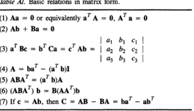
Table .41. Basic relations in matrix form.

(1) Aa = 0 or equivalently aYA = 0, AT"a = 0

(2) Ab + B a = 0 l al bi c l t (3) a T Be = b r C a = c t A b = I a2 b2 c2 l l a3 b3 c3l (4) A = b a r - (a Tb)I (5) ABA T = (a r b)A (6) (ABA T) b = B(AAr)b

(7) Ifc = Ab, thenC = AB - BA-- ba T - ab T

q = a r b and c = Ab. Many of the known vector identities can be derived by the use of the rules of matrix algebra involving only the representations of equations (A.1) and (A.2). Some o f the important basic relations (in matrix form) are given in table A1. Deriva- tion of these relations are rather elementary. Many other complicated but useful relations can be obtained by using them.

I f the use of more than one Cartesian coordinate system is of interest, it will be proper to indicate the representations in equations (A.1) and (A.2) by Sa and sA, respectively.

Therefore, in a different system, say ~, the same vector will be represented by ~a or zA, respectively, Let both S and r, be right-handed systems. Then these two different representations are interrelated by the following orthogonal transformations:

Sa = T ~:a ,g, SA = T(ZA)T T, _(A.3)

where the entries in the ith column of the 3 × 3 nonsingular transformation matrix T(t) correspond to the direction cosine o f the ith axis of ~ with respect to the axes of S. The orthogonal matrix T is in fact orthonormal, since I T f = 1:

T T T = T T T = I. (A.4)

The time derivative of both sides gives

0 l

T

(A.5)

(23)

A NETWORK M O D E L FOR RIGID-BODY MOTION 81

d T

=°

)J

(A.6)

then the relations in equations (A.5) become s t + stir = 0 and ~flr + r~fl = 0, respec- tively, which imply the skew-symmetric characters of s t and zfl [12, 20]. Note that the matrix products in equations (A.6) are, in general, not commutative; hence, the skew- symmetric matrices s t and gfl are different. In fact, it follows from equations (A.4) and (A.6) that

s t = T ~fl T T, (A.7)

which implies the existence of a spatial vector ~ (angular velocity) with the transformation property

so~ = T zoo. (A.8)

A similar relation can be shown to exist between the derivatives of s~ and ~o~:

d (so.,) = T d (~w). (A.9)

dt dt

Consider the relations in equation (15) with the superscripts removed:

Vi = V0 + floroi = Vo + R~ ~Oo, (A. 10)

where, in view of equations (10), the position vectors of the points B i and Ao are indicated by ri(= r~i) and r0(= ~ ) , respectively, and r0i = ri - r0 is fixed in the rigid body. Then the relation in equation (A.10) can be modified as

d d

R~/.6o 0 = V i -- V 0 = - - ( r i -- ro) = - - roi, (A.11)

dt dt

which allows one to write the skew-symmetric equivalent of the column matrix d/dt roi. Indeed, by the use of property 7 in table A1, we have

, 4

R 0 i = ~ a 0 - - a 0 R ~ -~- [~o R o i - PLOi n 0 = roi tOT - - 60o r T ,

dt

(A. 12)

from which we write

R o / d R o i = R o i ~'~o Roi - l ~ i [r~o = C -

R2i to.

dt

(24)

82 Y. TOKAD

The first term C = Roi flo Roi in the right-hand side of equation (A.13) is a skew- symmetric matrix that can be put into the following form by the use of property 5 in table AI:

C = Roi flo Roi = - (rT6oo)R0i • (A. 14)

or, in column matrix form,

c = r o , = - r o t = - ( r o , - 1

~ - - - [Ro i Rot -1- (roT/ roi) I] o~ o = Roi Ro r OJo - (r T roi) o~ o j~ (A. 15) = I i -- (r T rot) O:o,

where the property 4 in the table A1 and the definition I i = Rot 1~.~o o are used. Consider- ing again the third-order matrix, C, equivalent to c, equation (A.15) gives

C = L i - (r T roi)00. (A.16)

Substituting this expression into equation (A. 13) and again considering property 4 in table A1, we finally obtain the relation

R0 i d Ro i = Li _ (rot

roT/)

flo- (A. 17)

dt

The transpose of this relation also gives

Rol Roi = flo (rot rOT/) -- Li. (A.18)

On the other hand, using relation (A.12), an expression for the time derivative of the inertia matrix Jo can also be established as

d Jo = flo Jo - Jo flo- (A. 19)

dt

This relation follows from equations (21), (A.17), and (A.18):