OPTIMAL SIGNALING AND DETECTOR DESIGN FOR POWER CONSTRAINED
ON-OFF KEYING SYSTEMS IN NEYMAN-PEARSON FRAMEWORK
Berkan Dulek and Sinan Gezici
Department of Electrical and Electronics Engineering
Bilkent University, Bilkent, Ankara 06800, Turkey
{dulek,gezici}@ee.bilkent.edu.tr
ABSTRACTOptimal stochastic signaling and detector design are studied for power constrained on-off keying systems in the presence of additive multimodal channel noise under the Neyman-Pearson (NP) framework. The problem of jointly designing the signaling scheme and the decision rule is addressed in order to maximize the probability of detection without violat-ing the constraints on the probability of false alarm and the average transmit power. Based on a theoretical analysis, it is shown that the optimal solution can be obtained by employ-ing randomization between at most two signal values for the on-signal (symbol 1) and using the corresponding NP-type likelihood ratio test at the receiver. As a result, the optimal parameters can be computed over a significantly reduced op-timization space instead of an infinite set of functions using global optimization techniques. Finally, a detection example is provided to illustrate how stochastic signaling can help improve detection performance over various optimal and sub-optimal signaling schemes.
Index Terms— Stochastic signaling, on-off keying, Neyman-Pearson (NP) decision rule.
1. INTRODUCTION AND MOTIVATION
In power constrained binary communications systems, stochas-tic signaling; that is, modeling signals for transmitted symbols as random variables instead of deterministic quantities, can provide performance improvements in some scenarios [1, 2]. This method has proven effective in reducing the average probability of error for power constrained communications systems over additive noise channels with multimodal proba-bility density functions (PDFs).1
Although optimal signaling and detector design has been studied extensively in the literature according to various crite-ria (e.g., Bayes, minimax, Neyman-Pearson) when the noise is Gaussian, the noise can have significantly different proba-bility distribution than the Gaussian distribution in some cases due to effects such as multiuser interference and jamming [4]. Joint optimization of signal structures and detectors in terms of error performance is investigated under an average power constraint in [2]. It is proven that the optimal performance can be achieved when the transmitted signal for each symbol is randomized between no more than two signal values and the corresponding maximum a posteriori probability (MAP) detector is employed at the receiver. In [5], optimal random-ization among antipodal signal pairs and the corresponding MAP decision rules is studied under the assumption that the receiver knows which deterministic pair is transmitted. It is 1In [3], it is shown that if the channel has a continuously differentiable
unimodal PDF with finite variance, the average probability of error versus average power is a nonincreasing convex curve when the transmitter employs antipodal signaling, and the receiver uses the maximum likelihood (ML) rule. In that case, stochastic signaling cannot improve the error performance.
concluded that randomization between two detectors is suffi-cient to maximize the correct decision probability.
In detection theory, most of the research conducted on stochastic signaling has focused on improving the perfor-mance of detectors according to the average probability of error criterion [1, 2]. Although the prior probabilities of the symbols are assumed to be equal in many communications systems, they can be unknown and nonequal in certain cases [6]. Furthermore, it may not be possible to impose cost struc-tures on the decisions [7]. Under such scenarios, neither Bayesian nor minimax decision rules are applicable, and the Neyman-Pearson (NP) hypothesis testing provides a favorable alternative. For example, in wireless sensor network appli-cations, a transmitter can send one bit of information (using on-off keying) about the presence of an event (e.g., fire), in which case the probabilities of detection and false alarm be-come the main performance metrics as in the NP approach. In this study, we consider a power constrained on-off keying communications system in the NP framework, and formulate the problem of jointly designing the signaling scheme and the decision rule (detector). Based on a theoretical analysis, it is shown that the optimal solution can be obtained by employ-ing randomization between at most two signal values for the on-signal (symbol 1) and using the corresponding NP-type likelihood ratio test (LRT) at the receiver. Hence, the optimal parameters can be computed over a significantly reduced opti-mization space instead of an infinite set of functions. Finally, a detection example is provided to compare various optimal and suboptimal signaling schemes.
2. OPTIMAL SIGNALING AND DETECTOR DESIGN Consider an on-off keying communications system, in which the receiver acquiresM -dimensional observations over an ad-ditive noise channel and decides between the two hypotheses H0orH1, which are modeled as
H0 : Y = N , H1 : Y = S + N (1)
where Y is the noisy observation vector, S represents the transmitted signal for the alternative hypothesis (H1), and N
is the noise component that is independent of S. Instead of using a constant level for S as in the conventional case, one can consider a more generic scenario in which the signal S can be stochastic. Then, the aim is to find the optimal PDF for S in (1) and the corresponding decision rule that maximize the probability of detection under the constraints on the prob-ability of false alarm and average transmit power. A feedback mechanism from the receiver to the transmitter is assumed to facilitate the joint optimization of the signaling structure and the decision rule, which is a reasonable assumption, for exam-ple, for cognitive radio (CR) systems.
Note that the probability distribution of the noise compo-nent in (1) is not necessarily Gaussian. Due to interference, such as multiple-access interference, the noise component can have a significantly different probability distribution from the 2011 IEEE Statistical Signal Processing Workshop (SSP)
Gaussian distribution [8].
At the receiver, the structure of a randomized test is as-sumed to choose between the two hypotheses. Such a test is completely characterized by a decision ruleφ. For a given ob-servation vector y, this test accepts hypothesisH1with
prob-abilityφ(y), and rejects it with probability 1 − φ(y) where 0 ≤ φ(y) ≤ 1 for all y. If φ takes on only the values 0 and 1, the test reduces to a nonrandomized one, andφ simply becomes the indicator function of the decision region [9].
In the NP framework, for a given value of α ∈ (0, 1), the aim is to maximize the probability of detection such that the probability of false alarm does not exceed α. In other words, the tradeoff between type-I and type-II errors is taken into account in the NP approach [7]. Given the decision rule (detector)φ, the two probabilities of interest, the probability of detectionPDand the probability of false alarmPFA, can be
calculated as follows: PD= E1{φ(Y)} = Z RM φ(y) p1(y) dy PFA= E0{φ(Y)} = Z RM φ(y) p0(y) dy (2)
wherepi(y) denotes the conditional PDF of the observation
when hypothesis Hi is assumed to be true for i ∈ {0, 1},
and the subscripts on the expectation operators indicate the corresponding hypotheses. Since stochastic signaling is con-sidered, S in (1) is modeled as a random vector. Recalling that the signal and the noise are independent, the conditional PDF of the observation under the alternative hypothesisH1
can be calculated asp1(y) = RRMpS(x) pN(y − x) dx =
E{pN(y − S)} , where the expectation is taken over the PDF
of S. On the other hand, the conditional PDF of the ob-servation under the null hypothesis H0 is given simply by
p0(y) = pN(y). Then, using the linearity of the expectation
operator, the probability of detection can be expressed as PD= Z RMφ(y) E {p N(y − S)} dy = E ½Z RM φ(y) pN(y − S) dy ¾ , E {h(φ; S)} (3) and the probability of false alarmPFAis given by
PFA=
Z
RM
φ(y) pN(y) dy . (4)
In practical systems, there is a constraint on the average power emitted from the transmitter. Under the framework of stochastic signaling, this constraint on the average power can be expressed in the following form [7]:
EnkSk22
o
≤ A (5)
whereA denotes the average power limit.
One of the main motivations behind this study is to under-stand how stochastic signaling can help improve the detection performance of an on-off keying system without violating the constraint on the false alarm probability. Under the NP deci-sion criterion, the optimal signaling and detector design prob-lem can then be stated as
max {φ, pS} E{h(φ; S)} subject to PFA≤ α and E n kSk22 o ≤ A (6)
where the expectations are taken over the PDF of S, α ∈ (0, 1), and h(φ; S) and PFAare as in (3) and (4), respectively.
Note that there are also implicit constraints in the
optimiza-tion problem in (6), since pS(·) represents a PDF. Namely,
pS(x) ≥ 0 , ∀x ∈ RM, and
R
RMpS(x) dx = 1 should also
be satisfied by the optimal solution.
Although the optimization problem in (6) provides a generic formulation that is valid for any noise PDF, it is difficult to solve in general as the optimization needs to be performed over a space of signal PDFs and decision rules. In the following analysis, it is proven that optimizing over a set of variables (instead of functions) is sufficient to obtain the optimal signal PDF and the decision rule. To that aim, the following lemma is presented first.
Lemma 1: Given a decision ruleφ that satisfies the false
alarm constraint; ifh(φ; s) in (3) is a continuous function of s
defined on a compact subset ofRM, then an optimal solution
to(6) can be expressed in the form of
poptS (x) = λ δ(x − s1) + (1 − λ) δ(x − s2) , (7)
whereλ ∈ [0, 1].
Proof: Suppose that a decision rule ˜φ is given such that the constraint on the probability of false alarm is sat-isfied, i.e., RRMφ(y) p˜ N(y) dy ≤ α. Then, h( ˜φ; s) =
R
RMφ(y) p˜ N(y − s) dy in (3) becomes a function of s only.
Formally, PD in (3) can be represented asPD = E {h(S)}
and the optimization problem in (6) can be stated as max
pS
E{h(S)} subject to EnkSk22
o
≤ A . (8) Similar optimization problems have been studied extensively in the literature under various frameworks [1, 2, 5, 10]. Given the conditions in the lemma, Carath´eodory’s theorem from convex analysis [11] implies that the optimal solution of (8) can be expressed by a randomization of at most two signal vectors. Therefore, for any decision rule ˜φ satisfying the false alarm constraint, the optimal signal PDF can be represented as in (7).¥
At this point, it should be emphasized that the above lemma points out to a significant reduction on the complex-ity of the optimization problem under certain conditions. Namely, the optimal signal design no longer involves a search over all possible signal PDFs; but instead a randomization between at most two different signal vectors suffices. Hence, the problem in (6) can be solved over the signal PDFs that are in the form of (7). Led by this observation, a further simplification of the optimization problem is presented.
Proposition 1: Under the conditions in Lemma 1, the
op-timization problem in(6) can be expressed as follows: max {λ, s1, s2, η} Z Γ{λ p N(y − s1) + (1 − λ) pN(y − s2)} dy subject to Z Γ pN(y) dy = α λ ks1k22+ (1 − λ) ks2k22≤ A λ ∈ [0, 1] and η ≥ 0 (9) whereΓ = {y ∈ RM : λ p N(y − s1) + (1 − λ) pN(y − s2) > η pN(y)}, and α ∈ (0, 1) .
Proof: It is known that the NP detector gives the most powerfulα-level test of H0 versusH1 [7]. In other words,
when the aim is to maximize the probability of detection such that the probability of false alarm does not exceed a predeter-mined valueα, the NP detector is the optimal choice. When deciding between two simple hypothesesH0versusH1based
on observation y, the NP decision rule takes the following
form of an LRT: ˜ φN P(y) = 1 , if p1(y) > η p0(y)
γ(y) , if p1(y) = η p0(y)
0 , if p1(y) < η p0(y)
(10) whereη ≥ 0 and 0 ≤ γ(y) ≤ 1 are chosen such that the prob-ability of false alarm satisfiesPFA = E0{ ˜φN P(Y)} = α,
where the expectation is taken with respect to the null hy-pothesisH0. Then, the NP decision rule is the optimal one
among allα-level decision rules, i.e. PD = E1{ ˜φN P(Y)}
is maximized, where the expectation is taken with respect to the alternative hypothesis H1. It can be proven that such a
rule always exists for allα ∈ (0, 1) and is unique [7]. Let L(Y) = p1(Y)/p0(Y) be the likelihood function. For
con-tinuousL(Y), γ(Y) can be chosen arbitrarily since the prob-ability of the event{p1(Y) = η p0(Y)} is equal to 0 under
bothH0andH1[7, 9].
To keep the formulation simpler, the PDF of the chan-nel noise is assumed to be continuous which gives rise to a continuous likelihood function. An extension for the discrete case is straightforward by incorporating the parameterγ(y) into the calculations for the detection and false alarm proba-bilities. Under the continuity assumption, while deciding be-tween two simple hypotheses based on observation y, the NP decision rule, which selects hypothesisH1ifp1(y) > η p0(y)
and selects hypothesisH0otherwise, maximizes the
probabil-ity of detection under the false alarm constraint. Therefore, when the signal PDFpS(·) is specified, it is sufficient to
con-sider only the detection probability of the NP rule instead of a search over all the decision rules.
As the NP decision rule assigns observation y to hypoth-esisH1 ifp1(y) > η p0(y) and decides hypothesis H0
oth-erwise, the probability of detection and false alarm expres-sions in (2) can be expressed for an NP decision rule asPD=
E1{ ˜φN P(Y)} = RΓp1(y) dy and PFA = E0{ ˜φN P(Y)} =
R
Γp0(y) dy, where Γ =©y ∈ R M : p
1(y) > η p0(y)ª.
In Lemma 1, it is shown that an optimal signal PDF is in the form of (7). As a result, the conditional PDF of the observation under hypothesis H1 can be written as
p1(y) = E{pN(y − S)} =
R
RMpS(x) pN(y − x) dx =
λ pN(y − s1) + (1 − λ) pN(y − s2). Similarly, the average
power constraint in (6) becomesλ ks1k22+ (1 − λ) ks2k22 ≤
A . Therefore, the expressions for PDandPFA at the end of
the previous paragraph imply that the optimization problems in (6) and (9) are equivalent as stated in the proposition.¥
Proposition 1 implies that the solution of the original op-timization problem in (6), which considers the joint optimiza-tion of the stochastic signal PDF and the detector, can be ob-tained as the solution of the much simpler optimization prob-lem specified in (9).
Comparing the formulations in (6) and (9), it is noted that a significant complexity reduction is obtained in the represen-tation of the problem by optimizing over a set of variables instead of a set of functions. The solution of the optimization problem in (9) can be obtained via global optimization tech-niques (since it is not a convex problem in general), or a con-vex relaxation approach as in [12] can be employed to obtain approximate solutions in polynomial time. In this study, the multistart and patternsearch methods from MATLAB’s Global Optimization Toolbox are used to obtain the solution of (9).
Assuming that the selected optimization algorithm suc-cessfully returns the parameters©λopt, sopt
1 , s opt 2 , η
optª for
the problem in (9), the optimal signal PDF can be constructed
as poptS (x) = λ opt
δ(x − sopt1 ) + (1 − λ opt
)δ(x − sopt2 ),
and the optimal decision rule assumes the form of the cor-responding NP decision rule that decides hypothesis H1 if
λoptp N¡y − s opt 1 ¢ +(1−λ opt)p N¡y − s opt 2 ¢ > η optp N(y)
and decides hypothesisH0otherwise.
3. SIMULATION RESULTS AND CONCLUSIONS In this section, the optimal signal PDF and optimal detec-tor parameters are obtained by applying the theory devel-oped in the previous section along with the results from two closely related signaling techniques. A binary hypotheses-testing problem specified as in (1) is considered with scalar observations. Such a scenario is well suited for binary com-munications systems that transmit no signal for bit 0 and a signal (or a randomization of two signal values as dis-cussed above) for bit 1 (i.e., on-off keying). The noise N in (1) is modeled as a symmetric Gaussian mixture noise with equal variances, the PDF of which can be expressed as pN(n) =PLi=1liexp{−(n − µi)2/(2σ2)}/(
√
2π σ) [4]. It is noted that the average power of the noise can be calculated from E{N2
} = σ2+PL
i=1 liµ2i. Similar to those introduced
in [2], three different signaling schemes are considered. Conventional Solution: In this case, the transmitter employs deterministic signaling at the maximum permitted power level, which is known to be optimal if the noise present in the channel were Gaussian distributed. To mitigate the ef-fects of non-Gaussian channel noise, the receiver is assumed to know the channel statistics and allowed to design the op-timal NP decision rule corresponding to the deterministic signaling at the power limit. This optimization problem can be expressed as follows: max η Z Γ pN(y − A) dy s.t. Z Γ pN(y) dy = α , η ≥ 0 (11)
whereΓ = {y ∈ R : pN(y − A) > η pN(y)} and α ∈ (0, 1).
Optimal−Stochastic: This approach refers to the joint design of the signaling structure and the decision rule formu-lated in (6), which can also be obtained from (9) as studied in the previous section.
Optimal−Deterministic: A simplified version of the op-timal solution in (9) can be obtained by assuming that the transmitted signal is deterministic; i.e., it is not a randomiza-tion of two distinct signal levels. The optimizarandomiza-tion problem in (9) reduces to max {s, η} Z Γ pN(y − s) dy subject to Z Γ pN(y) dy = α , |s| 2 ≤ A , η ≥ 0 (12) whereΓ = {y ∈ R : pN(y − s) > η pN(y)} and α ∈ (0, 1).
In Fig. 1, the detection probabilities of the schemes de-scribed above are plotted versusσ for A = 1 and α = 0.05, where the parameters of the Gaussian mixture noise are given by l = [0.1492 0.1088 0.2420 0.2420 0.1088 0.1492] and µ= [−1.211 − 0.755 − 0.3 0.3 0.755 1.211].2
From the fig-ure, it is observed that the conventional solution has the worst performance as expected since no optimization is performed 2In obtaining the optimal solutions for the global optimization problems
stated above, MATLAB’s multistart method is employed with 250 random start points and sqp algorithm is used together with the local solver fmincon. The extrema returned by the method are cross-checked with the results from the patternsearch method. This procedure is repeated for all values of σ in the set{0.01 : 0.005 : 0.50}.
0 0.1 0.2 0.3 0.4 0.5 0.4 0.5 0.6 0.7 0.8 0.9 1 1.1 σ Pro b a b ili ty o f D e te ct io n , PD Conventional Optimal−Deterministic Optimal−Stochastic
Fig. 1. Probability of detectionPDversusσ for different
ap-proaches whenA = 1 and α = 0.05.
for the signaling scheme employed at the transmitter. As men-tioned above, signaling at the maximum permitted power level is not necessarily optimal for non-Gaussian cases. Having a multimodal PDF, channel noise degrades the performance of the communications system when the on-signal (symbol 1) is transmitted at the power limit. Optimizing deterministic sig-nal levels improves over the performance of the conventiosig-nal solution for0.01 ≤ σ ≤ 0.115 as observed from the Optimal– Deterministic curve by avoiding the overlaps among the com-ponents of the Gaussian mixture noise more effectively. Fur-ther performance improvements are obtained over a larger in-terval0.01 ≤ σ ≤ 0.20 when optimal stochastic signals are considered instead of conventional signaling (see Optimal– Stochastic). The superior performance of optimal stochastic signaling over optimal deterministic signaling is also evident from the values assumed by the probability of detection curves for0.04 ≤ σ ≤ 0.20. In contrast to finding the single sig-nal value that best avoids the overlaps among mixture compo-nents, stochastic signaling scheme allots the available power in such a way that a large portion of the power is allocated to the signal component that results in less overlap between the original and the shifted noise PDF on average. Hence, the best probability of detection performance is achieved by the solution of the joint optimization problem investigated in the previous section, which performs a randomization between two signal values for symbol 1, and employs the correspond-ingα-level NP decision rule at the receiver. For example, at σ = 0.1, the optimal stochastic signal is a randomization of s1 = 0.2732 and s2 = 1.2460 with λ = 0.3739, achieving
a detection probability of0.6494. On the other hand, the op-timal deterministic solution setss = 0.7684, resulting in a detection probability of0.5345.
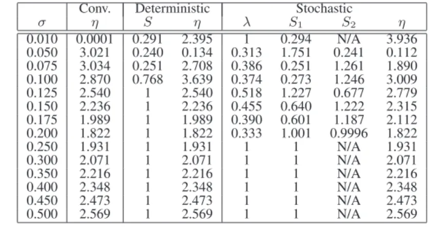
Asσ is increased beyond 0.20, it is observed that both op-timal signaling schemes converge to conventional signaling. This is mainly due to the fact that the overlap among mixture components of the noise PDF becomes significant for large values ofσ, and there is not enough freedom left for the ran-domization to become effective over transmitting at the power limit. It is also concluded from the results of the previous sec-tion that the performance figure achieved via randomizasec-tion is the global optimum; that is, it cannot be beaten by the combi-nation of any different signaling schemes with a single detec-tor as long as the problem formulation stays the same. In order to explain the results depicted in Fig. 1, Table 1 presents the solutions of the optimization problems in (11), (12), and (9) for the Conventional, Optimal–Deterministic and Optimal– Stochastic approaches, respectively. It is observed that Table 1 is in agreement with Fig. 1.
Conv. Deterministic Stochastic
σ η S η λ S1 S2 η 0.010 0.0001 0.291 2.395 1 0.294 N/A 3.936 0.050 3.021 0.240 0.134 0.313 1.751 0.241 0.112 0.075 3.034 0.251 2.708 0.386 0.251 1.261 1.890 0.100 2.870 0.768 3.639 0.374 0.273 1.246 3.009 0.125 2.540 1 2.540 0.518 1.227 0.677 2.779 0.150 2.236 1 2.236 0.455 0.640 1.222 2.315 0.175 1.989 1 1.989 0.390 0.601 1.187 2.112 0.200 1.822 1 1.822 0.333 1.001 0.9996 1.822 0.250 1.931 1 1.931 1 1 N/A 1.931 0.300 2.071 1 2.071 1 1 N/A 2.071 0.350 2.216 1 2.216 1 1 N/A 2.216 0.400 2.348 1 2.348 1 1 N/A 2.348 0.450 2.473 1 2.473 1 1 N/A 2.473 0.500 2.569 1 2.569 1 1 N/A 2.569
Table 1. Conventional, Deterministic, and Optimal-Stochastic Signaling
4. REFERENCES
[1] C. Goken, S. Gezici, and O. Arikan, “Optimal stochastic signaling for power-constrained binary communications systems,” IEEE Trans. Wireless Commun., vol. 9, no. 12, pp. 3650–3661, Dec. 2010.
[2] C. Goken, S. Gezici, and O. Arikan, “Optimal sig-naling and detector design for power-constrained binary communications systems over non-Gaussian channels,”
IEEE Commun. Lett., vol. 14, pp. 100–102, Feb. 2010. [3] M. Azizoglu, “Convexity properties in binary detection
problems,” IEEE Trans. Inform. Theory, vol. 42, no. 4, pp. 1316–1321, July 1996.
[4] V. Bhatia and B. Mulgrew, “Non-parametric likelihood based channel estimator for Gaussian mixture noise,”
Signal Processing, vol. 87, pp. 2569–2586, Nov. 2007. [5] A. Patel and B. Kosko, “Optimal noise benefits in
Neyman-Pearson and inequality-constrained signal de-tection,” IEEE Trans. Sig. Processing, vol. 57, no. 5, pp. 1655–1669, May 2009.
[6] I. Korn, J. P. Fonseka, and S. Xing, “Optimal bi-nary communication with nonequal probabilities,” IEEE
Trans. Commun., vol. 51, pp. 1435–1438, Sep. 2003. [7] H. V. Poor, An Introduction to Signal Detection and
Es-timation, Springer-Verlag, New York, 1994.
[8] T. Erseghe, V. Cellini, and G. Dona, “On UWB impulse radio receivers derived by modeling MAI as a Gaussian mixture process,” IEEE Trans. Wireless Commun., vol. 7, no. 6, pp. 2388–2396, June 2008.
[9] E. L. Lehmann, Testing Statistical Hypotheses, Chap-man & Hall, New York, 2 edition, 1986.
[10] H. Chen, P. K. Varshney, S. M. Kay, and J. H. Michels, “Theory of the stochastic resonance effect in signal de-tection: Part I–Fixed detectors,” IEEE Trans. Sig.
Pro-cessing, vol. 55, no. 7, pp. 3172–3184, July 2007. [11] R. T. Rockafellar, Convex Analysis, Princeton University
Press, Princeton, NJ, 1968.
[12] S. Bayram, S. Gezici, and H. V. Poor, “Noise en-hanced hypothesis-testing in the restricted Bayesian framework,” IEEE Trans. Sig. Processing, vol. 58, no. 8, pp. 3972–3989, Aug. 2010.