THE INFLATION TAX AND PERIOD LENGTH IN CASH-IN-ADVANCE MODELS A Master’s Thesis by BEDRİYE ÇUBUK Department of Economics Bilkent University Ankara July 2002
THE INFLATION TAX AND PERIOD LENGTH IN CASH-IN-ADVANCE MODELS
The Institute of Economics and Social Sciences of
Bilkent University
by
BEDRİYE ÇUBUK
In Partial Fulfilment of the Requirements for the Degree of MASTER OF ECONOMICS in THE DEPARTMENT OF ECONOMICS BILKENT UNIVERSITY ANKARA July 2002
I certify that I have read this thesis and have found that it is fully adequate, in scope and in quality, as a thesis for the degree of Master of Economics.
Assist. Prof. Dr. Neil Arnwine Supervisor
I certify that I have read this thesis and have found that it is fully adequate, in scope and in quality, as a thesis for the degree of Master of Economics.
Assist. Prof. Dr. Erdem Başçı Examining Committee Member
I certify that I have read this thesis and have found that it is fully adequate, in scope and in quality, as a thesis for the degree of Master of Economics.
Assist. Prof. Dr. Levent Akdeniz Examining Committee Member
Approval of the Institute of Economics and Social Sciences
Prof. Dr. Kürşat Aydoğan Director
ABSTRACT
THE INFLATION TAX AND PERIOD LENGTH IN CASH-IN-ADVANCE MODELS
Çubuk, Bedriye
M.A., Department of Economics Supervisor: Assist. Prof. Neil Arnwine
July 2002
The aim of this study is to focus on the frequency with which consumers conduct financial transactions, and the role that this plays in the determination of the money velocity, price level, transactions cost and consequently determination of welfare cost of inflation. We introduce a CIA model with a Baumol-Tobin transactions mechanism. This provides a contribution to the CIA literature by allowing the transactions period to be endogenous and contributes to the Baumol-Tobin model by placing the decision rules in a general equilibrium setting. We find that the transactions period length is an integral part of the behavior of the monetary economy.
Keywords: Cash-in-advance Models, Transactions Cost, Velocity of Money,
ÖZET
ENFLASYON VERGİSİ VE NAKİT KISITLARININ OLDUĞU BİR EKONOMİDE PERİYOT UZUNLUĞU
Çubuk, Bedriye Master, Ekonomi Bölümü
Tez Yöneticisi: Y. Doç. Dr. Neil Arnwine
Temmuz 2002
Bu çalışmanın amacı, tüketicilerin finansal işlem yapma sıklığını incelemek ve bu sıklığın paranın dolaşım hızı, fiyat düzeyi, işlem maliyeti ve sonrasında enflasyonun refah düzeyi üzerindeki etkilerini incelemektir. Baumol-Tobin işlem mekanizması olan, satınalmalarda nakit kısıtlarının bulunduğu bir model geliştirdik. Bu model, işlem periyodunda değişime izin vererek nakit kısıtlarının olduğu modellere, genel denge içerisinde karar verme özelliğiyle de Baumol-Tobin modellerine katkıda bulunmuştur. İşlem periyot uzunluğunun parasal ekonomide önemli bir yer aldığını gözlemledik.
Anahtar Kelimeler: Nakit Kısıtlı Modeller, İşlem Maliyeti, Paranın Dolaşım Hızı,
ACKNOWLEDGMENTS
I would like to express my deepest gratitude to Assist. Prof. Dr. Neil Arnwine for his endless patience and excellent supervision. His great guidance lead me to this point. I am very thankful to Assist. Prof. Dr. Erdem Başçı for his invaluable comments. I also wish to thank to Assist. Prof. Dr. Levent Akdeniz for his comments.
I am indebted to a number of friends Çiğdem G. Yılmaz, Özlem Güner, Özgü Serttaş and Sezin Kösoğlu.
I owe special thanks to my great family for their everlasting supports and patience. Their encouragements and every sort of support have helped me to come to this point. Truly thanks to Makbule and Sezai who have always kept their belief in me, I always felt their support.
The most thanks go to Serdar especially for his patience and understanding. I could not have succeeded without his support. Thank you for everything, Serdar. Thank you for being beside me.
TABLE OF CONTENTS
ABSTRACT……… .iii
ÖZET……… …iv
ACKNOWLEDGMENTS………vi
TABLE OF CONTENTS……… …vii
CHAPTER I: INTRODUCTION………...1
CHAPTER II: THE MODEL……….7
2.1 Equilibrium Concept……….…7
2.2 The Government………...8
2.3 Consumer Constraints………...8
2.4 The Firm……….……….11
2.5 Value Function………12
2.6 First Order Conditions (FOC)………...12
2.7 Combining the First Order Conditions………13
CHAPTER III: CALIBRATION AND NUMERICAL SOLUTION………...16
3.1 Calibration………...16
CHAPTER IV: FRIEDMAN RULE ………...18
CHAPTER V: RESULTS………..21
5.1 Velocity…...……….…21
5.2 The Seigniorage………...23
5.3 Transactions Cost……….26
5.4 Does Timing Matter? ………..28
CHAPTER VI: CONCLUSION………33
1
INTRODUCTION
In typical cash-in-advance (CIA) models, the transactions period length is considered to be fixed and exogenously determined. In empirical work this assumption is strengthened by fixing the period length to be consistent with the frequency of data collection. We relax this restriction by allowing the consumer to jointly choose the initial money stock and frequency of transactions just like Baumol (1952)-Tobin (1956) to satisfy the CIA constraint.
We introduce a flexible transactions technology into the standard CIA model of money demand. With this innovation1, we generalize the determination of the velocity of money in the general equilibrium CIA model. The consumer balances the opportunity cost of holding money with the cost of transacting τ * n where τ is the marginal cost (possibly “shoe-leather”) of transacting and n is the number of trips to the bank.
In the first CIA model introduced by Lucas (1980), consumers learn the state of the economy before they trade assets and money, so they hold exactly enough money to facilitate their purchases, hence the velocity of money is forced to be unity. Several works have tried to relax this result. Lucas (1980) and Svensson (1985) relax this result by introducing uncertainty into the model. In these models, money balances are selected before the state of the world is known. In Lucas (1980) there is
uncertainty about demand for consumption good, in Svensson (1985) there is uncertainty about money growth, and therefore about the price level. In these models it is possible for the CIA constraint to be slack in some periods, so the velocity may vary below unity. Lucas and Stokey (1987) introduced a model with “cash” and “credit” goods. This innovation in the model allows the velocity of money to vary above unity because total purchases may be greater than money balances.
The literature on money velocity is not new. Baumol (1952) analyzed the transactions demand for cash for the rational consumer who wants to balance the opportunity cost of holding money, foregone interest, with the cost of obtaining new money balances via costly transactions. He focused on a steady state environment where precautionary and speculative demands have no place. Using Baumol’s notation, the consumer has to pay out T amount of cash in a determined period of time. He has to minimize on the sum of broker’s fees and the opportunity cost of holding cash. Baumol derived the square root formula for demand for cash to be C = (2*b*T/i)1/2 , where C is the withdrawal amount, b is the “brokerage fee”, T is the total payment, and i is the interest rate. Given the price level, the demand for cash is proportional to the square root of the value of the transactions. The Baumol model depicts the non-coincidence of discrete cash receipts and payments which occur in a steady stream. In a similar model, Tobin (1956) found that
“…the failure of receipts and expenditures to be perfectly synchronized certainly creates the need for transactions balances.” (page 241)
In his case the transactions fee consists of two, namely, constant and variable parts. The problem he encounters is to find the relationship between the average bond holding and the interest rate, where cash and bond holding are the choice variables, to maximize the after transactions cost interest revenue.
Rodriguez (1998) inserts Baumol and Tobin’s setup into a general equilibrium CIA model where the velocity of money is calculated within the model. In his model, the consumer economizes on his cash holdings by altering the number of trips to the bank with the changing inflation. Except from the first transaction, there is a fixed cost of transacting. The consumer chooses his bond holdings and the amount of the withdrawal for the succeeding period. A precautionary demand for money is obtained and the variability of velocity above unity is achieved. In his paper, Rodriguez concludes that the results of the deterministic models are very close to the stochastic ones.
Corbae (1993) allows variation in velocity by allowing consumers to relax the CIA constraint by incurring a fixed transactions cost. As it is usual in CIA models, the transactions period is exogenously determined so there is not a true trade-off between holding money balances and transacting as in Baumol-Tobin model.
The empirical performance of the CIA models is linked to the data period. The data frequency is generally predetermined to be a quarter, which implicitly imposes that the consumer’s cash holding will last for 13 weeks. Giovaninni and Labadie (1991) examine the performance of the CIA models find that for a number of parameter combinations the CIA constraint always binds and allows no variations
in the velocity. We assert that this results from the assumption that the finance period was assumed to be exogenous and fixed. Hodrick, Kocherlakota, Lucas (1991) also explore whether the mentioned models can produce realistic predictions. They find that in the cash-only model, the predicted velocity of money is always constant and unitary. In the cash-credit model, velocity varies as agents can substitute between cash and credit goods. Using a model with Svensson’s timing assumption, their model could not satisfactorily explain the observed variability of velocity.
Other empirical work using the CIA model has shown the deficiency in the model. Cooley and Hansen (1989) simulated a CIA model which is calibrated for both quarterly and monthly data, which includes leisure and investment decisions for studying the welfare costs of inflation. In the monthly case the welfare cost of inflation predicted by the model is significantly lower than in the quarterly case. This again points out the existence of a problem in the concept of transactions period length in CIA models. Their result is to be expected. For a given stock of money, a CIA constraint placed upon a quarter’s purchases should bind much stricter than a CIA constraint placed upon a month’s purchases. Therefore the predicted utility cost of inflation is higher in the quarterly model. This is a case of model failure.
In Cooley and Hansen (1989) the only way that consumers can reduce the cash holdings in response to the high inflation is to reduce consumption, which increases consumption of other goods, leisure and investment. In a latter work, Cooley and Hansen(1991) introduce a production economy utilizing Lucas and Stokey’s cash credit model with Svensson’s timing convention. In this study, Cooley
and Hansen compare the welfare cost of income and capital taxes with those of an inflation tax. Quoting from the paper:
" Choosing a measure of money presents problems. Conventional monetary aggregates that one might use to capture quantities subject to the inflation tax- the monetary base, or the non-interest bearing portion of M1- have the drawback that they are too large. They imply velocities less than unity which is inconsistent with the model. Instead, we use the portion of M1 that is held by households." (page 492)
When new data series must be constructed to confirm to the model, there is a problem with the model.
In this work, we endogenize the transactions decision. We mainly follow Cooley and Hansen (1991) for comparison purposes. After calibrating the model to match observed velocity we replicated Cooley and Hansen’s (1991) “inflation tax only” model. We find the velocity of money is determined within the model and can vary in response to the high inflation. Our results2 show that the velocity can take values both below and above unity within the same model. This result has not been shown before.
The work is organized as follows; Chapter II introduces the model, Chapter III describes how the model is calibrated and solved numerically, Chapter VI explains the Friedman Rule which is the benchmark case for comparing the welfare
effects of inflation on the economy. Chapter V presents the results. Chapter VI concludes.
2. THE MODEL
We study an economy which consists of a representative competitive firm, which rents capital and hires labor to produce output using a Cobb-Douglas production technology. The model used will be the same as that examined in Cooley and Hansen (1991) with the innovation of period length in the cash-in-advance constraint. In this study, we concentrate on the properties of the steady-state, non-stochastic, equilibrium.
2.1 Equilibrium Concept
In this model the firm produces output and facilitates costly transactions for the consumer. Both functions are conducted on a competitive basis. During a transaction the firm provides the consumer with cash. Between transactions cash flows from the consumer to the firm as the consumer purchases the cash good.
The transactions fee can be considered as the cost of confirming that the consumer’s budget constraint can support the cash withdrawal and recording the transaction. The existence of such a cost motivates the existence of a cash based transactions mechanism.
2.2 The Government
The sole role of government in this economy is to supply money. Money is supplied to the economy via lump sum transfers, or tax, of TR=M′−M =
(
g−1)
⋅M , where g is the growth rate of money balances3.2.3 Consumer Constraints
The cash-credit good model of Lucas and Stokey (1987) is adopted. The model does not include any uncertainty and all markets are competitive. The representative consumer maximizes the utility function; U (c1, c2, h) given in equation 1.
(
h)
( ) (
) ( )
hU c1,c2, =αlogc1 + 1−α logc2 −γ⋅ (1)
Here, c1 is the consumption of “cash good” and c2 is the consumption of “credit
good”, α is the relative weight given to the consumption of the cash good in the utility function. Labor hours, h, enter the utility function linearly. This incorporates the concept of Hansen (1985) in which an employment lottery is used to linearize the utility effect of employment.
The representative consumer faces the budget constraint, presented in real terms, given in equation 2:
p TR p m k r h w n p m i c c1+ 2+ + ′+ ⋅τ≤ ⋅ + ⋅ + + (2)
The consumer receives labor income expressed as the wage rate multiplied by hours worked, w⋅h, and rental income on capital, r⋅k, where r is the rental rate and
k is the stock of capital. Real money balances,
p m
, were selected in the previous
period and these are augmented by the lump sum transfer of new money added to the system,
p TR
. The assets listed on the right hand side of equation 2 are divided among
the following uses: consumption of the cash good, c1, and credit good, c2, investment into new capital, i, real money balances selected for the next period,
p m′
,
and transactions costs, n⋅τ, where n is the number of transactions per data period and τ is the cost per transaction.
The demand for money is motivated by a cash-in-advance constraint. In the benchmark example new transfers are not available as liquidity. This is presented in real terms in equation 3:
p n m
c1≤ ⋅ . (3)
The innovation of the model is the introduction of the velocity variable, n, representing the number of transactions per period, and the associated cost of transacting is given by τ. This brings in the contribution of Baumol-Tobin in which the consumer jointly decides both the stock of money to carry and the frequency with
which that stock is replenished. If we set n = 1 and τ = 0 then the model is the same as Lucas and Stokey (1987). This model is also utilized in Cooley and Hansen's (1991) 'Inflation Tax Only' case. The variable n is interpreted as the velocity of money in the data period. The velocity can take any non-negative value. The timing used in equation 3 is the same as the timing of Svensson (1985) that is the supply of money is not available before the next period. Although this timing convention sometimes leads the CIA constraint to strictly bind in Svensson's model, the innovation, n, relaxes the CIA constraint in this model. The case where the new money supply is available used in the same period is also examined.
The law of motion for the capital stock is: k′ 1=
(
−δ)
k+i. There is an economy-wide resource constraint which binds in equilibrium; the agent can not spend more than the period output, it is either consumed, invested as physical capital, or used up in a transaction: c1+c2+i+τ⋅n≤ y. In equilibrium, the resource constraint, budget and CIA constraints will all hold with equality, because the consumption good is always valued.To simplify the problem we introduce a transformation of variables:
M m mˆ = and M g p M p p ⋅ = ′ = ˆ
where m is representative consumer's money demand and M is the average money supply, so mˆ is the relative share of money held by the representative consumer. In
money balance, mˆ, is the numerairé in this model which will be unity at equilibrium. After the substitution of variables the utility function can be written:
(
)
(
)
(
)
τ ⋅ − ′ − ′ − δ − + ⋅ − − − + ⋅ + ⋅ ⋅ ⋅ = n h p m k k g p m n g k r h w g p n m U h c c U , ˆ ˆ 1 ˆ ˆ 1 1 , ˆ ˆ , , 2 1 . (4) 2.4 FirmThe firm produces output according to a constant returns to scale, Cobb-Douglas production function:
(
K H)
K H FY = , = θ 1−θ (5)
Since input markets are competitive, the wage is given by the marginal product of labor:
(
) (
)
θ − = θ H K H K W , 1 , (6)the rental rate of capital is:
(
)
θ = − θ H K H K R 1 , . (7)Capital letters refer to variables outside of the representative consumer's control and small letters refer to the consumer's choice variables. In equilibrium all markets clear, so h=H,k =K,i =I ect.
2.5 Value Function
The consumer's utility maximization problem can be represented as a value function: v
(
k m)
{
u(
c c h)
v(
k m)
}
n m k h + ′ ′ = ′ ′ , , , max , 1 2 , ˆ , , β (8)Since there is no uncertainty, it is not necessary to consider v
(
k′,m′)
as an expectation. Each period the consumer selects the labor supplied, the amount of capital stock to carry forward, the amount of money stock to carry forward, and the number of transactions to undertake given the current income and real money balances determined in the previous period.2.6 First Order Conditions (FOC)
The first order conditions for the consumer's problem are:
(
1)
0 0 2 2 2 = γ − α − = = ∂ ∂ + ∂ ∂ ∂ ∂ = c w h u c u h c vh (9)(
)
(
)
( )
1 1(
,)
0 0 , , 2 2 2 = ′ ′ + − − = = ′ ′ + ∂ ∂ ′ ∂ ∂ = ′ ′ ′ m k v c m k v c u k c m k v k k k β α β (10a)(
)
(
)
(
,)
0 1 ˆ 1 0 , ˆ , ˆ 2 ˆ 2 2 ˆ = ′ ′ + − − = = ′ ′ + ∂ ∂ ′ ∂ ∂ = ′ ′ ′ m k v c p m k v c u m c m k v m m m β α β (11a) 0 1 ˆ ˆ ˆ ˆ 0 2 1 2 2 1 1 = −α τ + ⋅ − α ⋅ = = ∂ ∂ ∂ ∂ + ∂ ∂ ∂ ∂ = c c c c c c v g p m g p m u n u n nWe can use the envelope theorem to eliminate vk′
(
k′,m′)
and vmˆ′(
k′,m′)
:(
)
−α δ − + = ∂ ∂ ∂ ∂ = c c c v u r k k 2 2 2 1 1 (10b) −α ⋅ − − α ⋅ = ∂ ∂ ∂ ∂ + ∂ ∂ ∂ ∂ = c c c c c c v g p n g p n u m u m m 2 1 2 2 1 1 ˆ 1 ˆ 1 ˆ ˆ ˆ (11b)2.7 Combining the First Order Conditions
In this model the solution for the production decisions h, k′ and y is separate from the consumption decision and is not effected by the money supply process. The
production component of the model has been included in our economy for easy comparison with Cooley and Hansen(1991).
Equilibrium capital stock is found by iteration. Combining FOC we obtain simple consumption rules:
(
)
τ α − − ⋅ = y i n c1 and(
)(
y i)
c2= 1−α − .Notice that consumption of credit good is invariant with respect to the number of transactions, and therefore with respect to the inflation rate. This results from the linear inclusion of labor in the utility function. When inflation increases consumer tends to transact more to economize on his money holdings. Transactions costs reduce the consumption of c1 so drives a wedge between the marginal utility of c1
and c2.
The price level and the velocity of money, n, are determined jointly by the following two equations:
+ − β ⋅ α γ = − − g n g W pˆ 1 1 (12)
( )
[
]
(
)
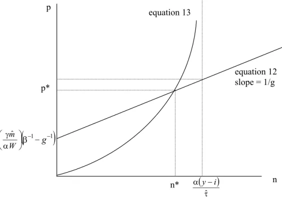
τ − α < < τ ⋅ − − α = − n y i g n n i y pˆ 1 , 0 (13)Equation 12 shows a stationary equilibrium with respect to mˆ.In this equation pˆ increases linearly in n. Equation 13 gives combinations of pˆ and n which satisfy resource constraints. Figure I shows graph of equation 12 and 13. In equation 12 we restrict ourselves to stationary equilibrium and the graph shows that there is a unique solution for n ≥ 0 and pˆ≥ 0and for g ≥ β. Equation 12 is linear, at n = 0 the slopes of equations 12 and 13 are equal and the slope of equation 13 is increasing in n. Also,
(
)
τα y i /
n= − provides a vertical asymptote to equation 13. Hence, there is a unique solution for g ≥ β. If g < β there is no solution with positive price.
Figure 1: Unique Solution when g≥β
(
g)
W mˆ −1− −1 α γ β equation 13 n* p* p equation 12 slope = 1/g n(
)
τ − α ˆ i y3. CALIBRATION AND NUMERICAL SOLUTION
3.1 Calibration
All parameters of the model, except for τ, are chosen to be the same as Cooley and Hansen (1991) for comparison purposes. The share of capital in total output, θ, is 0,36. The quarterly depreciation rate, δ, is set to be 0,02. The discount factor, β, is equated to 0,99 where annual real inflation rate is 4 percent. The coefficient of labor supplied in the utility function, γ, is 1,8 and α, the relative importance of cash and credit good in the utility function, is 0,844.
We calibrate the transactions cost τ so that the model replicates U.S. money velocity for the observation period using the money growth rate, g, which matches the observed inflation rate.
Considering the recent technological innovations in money sector, we adopted quarterly data from 1981,1 to 2000,4 on real GDP, money stock, consumption, capital stock, and the CPI for our calculations. The inflation rate between the specified periods is found to be % 0,8 using CPI data.
Monthly money supply (not seasonally adjusted) data aggregated in to quarters is used. The average quarterly M1 and M2 velocity for U.S. in the specified period is found to be 1,78 and 0,47, respectively. In our model this velocity is interpreted as the number of transactions conducted by the consumer, n, for U.S. in the past 20 years period. We find that τ is 0.0068 for M1 and 0.0951 for M2.
3.2 Numerical Solution
Since the model can not be solved analytically, we solved it numerically by using Gauss program. The only variable is the inflation rate. By changing the annual inflation rate we examine the change in consumption, velocity, prices, seigniorage revenue and transactions cost.
4. FRIEDMAN RULE
Money as a medium of exchange satisfies the double coincidence of wants and makes transacting easier. Though it is essential for carrying out some transactions, money can be costly to hold. While many other sorts of investment vehicles pay interest, most forms of money, such as currency, pay little or no interest. In order to decide how much money to hold, consumers must balance the costs of the foregone interest payment with the saved transaction cost.
Milton Friedman (1969) described the optimal inflation rate as one that does not penalize the consumer for holding money that pays no interest. This would require a zero nominal interest rate. Using Fisher’s relationship between nominal and real interest rates;
( ) (
1+i = 1+r)(
1+π)
, we can see that, the real return on money must be the negative of the inflation rate(
1+r) (
= 1+π)
−1.In our model the money growth rate, g, is also the inflation rate as there is no real output growth. The Friedman Rule, g = β, is used as a benchmark for utility loss due to inflation. When g=β the nominal interest rate is zero and the consumer is indifferent to holding money. As g approaches β from above, n goes to zero. Utility is maximized when g = β. At this point, there is no loss of resources due to
measure of welfare losses associated with inflation is computed. The welfare cost is measured by x in equation 14 where U* is the utility under Friedman Money Growth Rule. Here, x is the proportion increase in goods c1 + c2 required to restore utility
lost due to inflation. This is the method employed by Cooley and Hansen (1991).
U* = α log [ c1 (1+x)] + (1-α) log [c2 (1+x)] - γ h (14)
We find that x is strictly increasing in g. Inflation reduces utility.
We compute ∆C= x
(
c1+c2)
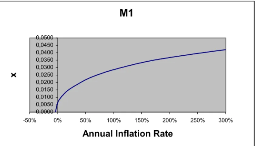
/y, where C∆ is the total change in consumption required to make the consumer as well off as under the Pareto optimal allocation as a percentage of GDP. Column A in Table 1 and Table 2 gives values ofx for M1 and M2 respectively and column B gives ∆C.
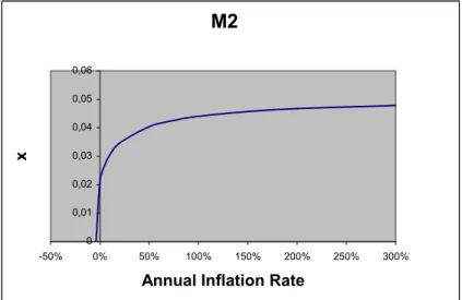
Figure 2 and Figure 3 graph the relationship between x and inflation rate. Figure 2 is for the M1 calibrated model and Figure 3 is for the M2 calibrated model. In the both figures the marginal cost of inflation is very high in low inflation rates.
M1 0,0000 0,0050 0,0100 0,0150 0,0200 0,0250 0,0300 0,0350 0,0400 0,0450 0,0500 -50% 0% 50% 100% 150% 200% 250% 300% Annual Inflation Rate
x
Figure 2: Welfare Loss of Inflation (Model Calibrated to Fit M1 Data)
M2 0 0,02 0,04 0,06 0,08 0,1 0,12 0,14 0,16 0,18 0,2 -50% 0% 50% 100% 150% 200% 250% 300% Annual Inflation Rate
x
5. RESULTS
We numerically solve the calibrated model and analyze the effects of different annual inflation rates on price levels, seigniorage revenue, transactions cost and the velocity of money. The results for M1 data are presented in Table1 and the results for M2 are presented in Table2.
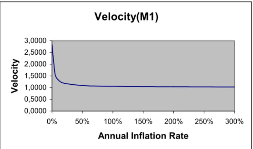
5.1. Velocity
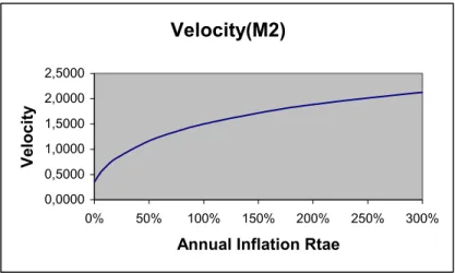
A major result of this paper is the fact that the velocity of money, defined as the number of transactions per data period, n, is not forced to be either unity, or less than or greater than unity. When the consumer economizes on his cash holdings he can change the number of transactions he will encounter. In the model, velocity of money increases with inflation, which is consistent with Baumol-Tobin's predictions. Due to the calibration, our model is able to exactly match the average M1 and M2 velocities to U.S. data. Observe that in Table 2 the M2 velocity takes values which are both below and above unity, depending on the inflation rate. This result has not been achieved before as the previous models always restricted the velocity of money as discussed in section 1.
At low rates of inflation, the marginal impact of inflation is very powerful on velocity, seigniorage revenue, price level and transactions cost. For those inflation rates, the consumer sharply increases his number of transactions to be able to reduce
his cash holdings. For higher rates of inflation the number of transactions continues to increase but the response to the inflation change is not so rapid.
Velocity(M1) 0,0000 2,0000 4,0000 6,0000 8,0000 10,0000 0% 50% 100% 150% 200% 250% 300%
Annual Inflation Rate
Velocity
Figure 4: Change in Velocity With Inflation (Model Calibrated to Fit M1 Data)
Velocity(M2) 0,0000 0,5000 1,0000 1,5000 2,0000 2,5000 0% 50% 100% 150% 200% 250% 300%
Annual Inflation Rtae
Velocity
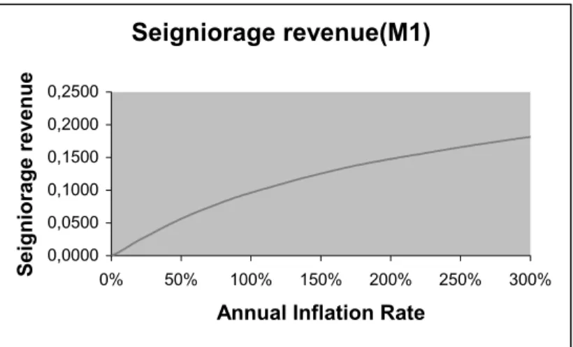
5.2 The Seigniorage
The government can finance its spending in three ways; apply direct taxes, borrow from public, or print money. Although, seigniorage, the government revenue raised by creating money, is a relatively cheap way of financing, it also results in social costs. When government finances its spending with the new issued money, it increases the money supply. Money growth leads the consumers to expect inflation at the rate of money growth. Inflation raises the opportunity cost of holding money. Consumers tend to economize on their money holdings. In equilibrium, the price level will be higher and the transactions will lead to a friction, which drives a wedge between marginal utilities of consumption of c1 and c2, cash and credit good,
respectively.
Inflation transfers the purchasing power from the consumer to the government. Hence, seigniorage resulting in inflation works as a tax on money holdings. As a quantitative literature states seigniorage revenue alone can not be sufficient enough to cover government spending5. Imrohoroglu and Prescott (1991) and Haslag (1998) emphasize this as:
“ ..if government were to make purchases; if it has to cover its spendings, seigniorage tax is not a good one relative to a tax on labor income.”
“For the most countries, money creation accounts for less than 2 percent of real GDP. The evidence indicates that seigniorage revenue is not the primary
5 For the discriptions I have benefited from the FRBSF Economic Letters of Marquis(2001) and
source of revenue for a government, but neither is it quantitatively insignificant.”
In our model, the government does not make any purchases. Seigniorage revenue is transferred to the consumer in lump sums. By printing money the government lowers the value of pre-existing money. We have examined two timing conventions. In the first one the newly issued money is not available as cash for spending in the same period, in the second one this money is available to spend in the same period.
Seigniorage, as a tax on holding money, has direct and indirect effects on welfare. The transactions cost will effect the consumer directly by reducing resources available for other ends. Seigniorage also drives a wedge between the marginal utilities of the cash and credit goods.
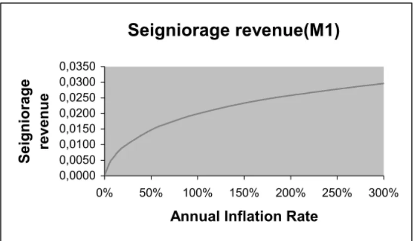
The seigniorage revenue raised is shown in Figure III and Figure IV for M1 and M2 data respectively. The marginal seigniorage revenue when annual inflation rate is low is very high when compared with higher rates of inflation.
Seigniorage revenue(M1) 0,0000 0,0050 0,0100 0,0150 0,0200 0,0250 0,0300 0,0350 0% 50% 100% 150% 200% 250% 300%
Annual Inflation Rate
Seigniorage revenue
Figure 6: Seigniorage Revenue As a Function of Inflation (Model Calibrated to Fit M1 Data) Seigniorage revenue(M2) 0,0000 0,0200 0,0400 0,0600 0,0800 0,1000 0,1200 0% 50% 100% 150% 200% 250% 300%
Annual Inflation Rate
Seigniorage revenue
Figure 7: Seigniorage Revenue As a Function of Inflation (Model Calibrated to Fit M2 Data)
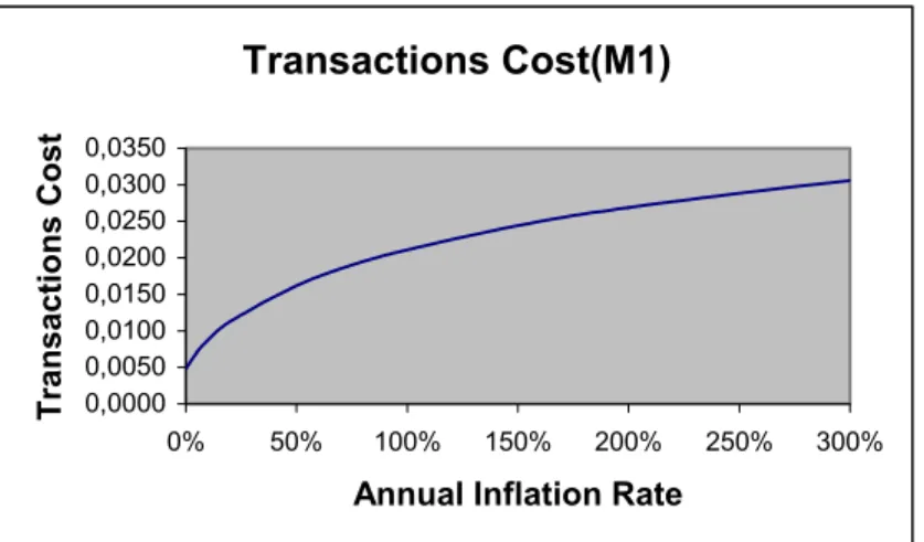
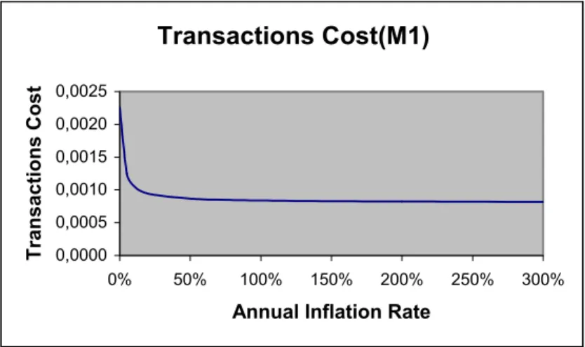
5.3 The Transactions Cost
As in Baumol-Tobin, the inflationary environment increases transacting and therefore transactions costs. Inflation can divert the resources allocated for consumption to the payment systems. When facing higher inflation, consumers economize on their money holdings. As inflation rises, a bigger percentage of the economy’s resources go into transacting in such ways so less will be available for production, thus reducing output and consumption and lowering welfare. The C column in Table 1 reflects the results of transactions cost, τ * n, as a percentage of GDP.
As the inflation rate increases, the transactions cost increases and the welfare declines. The decrease in welfare has two interpretations; (1) resources are lost when transacting and (2) transacting drives a wedge between the marginal utilities of c1
and c2. In higher rates of inflation, the wedge between consuming cash and credit
good gets bigger. It appears from our results that the predominant cost of inflation is the transactions cost as opposed to the reallocation of goods between c1 and c2.
Looking to Table 1 it is clear that B and C columns, the welfare cost and the transactions cost, respectively, are pretty similar. Only with very high inflation rates, we find that the values in column B are slightly bigger than those in column C. This reflects the additional welfare loss due to the fact that the transactions cost affect only one good.
Transactions Cost(M1) 0,0000 0,0050 0,0100 0,0150 0,0200 0,0250 0,0300 0,0350 0% 50% 100% 150% 200% 250% 300%
Annual Inflation Rate
Transactions Cost
Figure 8: Transactions Costs With Inflation (Model Calibrated to Fit M1 Data)
Transactions Cost(M2) 0,0000 0,0200 0,0400 0,0600 0,0800 0,1000 0,1200 0,1400 0% 50% 100% 150% 200% 250% 300%
Annual Inflation Rate
Transactions Cost
5.4 Does Timing Matter?
We also checked to see whether the timing of the transfer payment matters for the consumer when giving his consumption decisions. When the transfer payment is added to equation (3), the consumer will have the opportunity to use the transfer in the same period not only for the credit good but also for the cash good. The results with this set up are summarized in Table 3 with M1 calibrated data and in Table 4 with M2 calibrated data.
The results show that timing of transfer payments matters. Figures from 10 to 17 depicts the graphs of welfare cost of inflation, velocity of money, seigniorage revenue and transactions costs with this timing change and with M1 and M2 calibrated models. Under this timing convention, as inflation rises, the velocity of money converges to one. In the case of the M1 calibrated model, the convergence is from above one so transactions are predicted to fall as inflation rises. Therefore, the welfare loss due to inflation decreases in higher inflation rates. With the M2 calibrated model, the velocity converges to one from below so the welfare cost is increasing in inflation again. This timing convention is unattractive because it implicitly makes the data period important for the consumer. Each data period the consumer receives a transfer,
p TR
. This can not be converted into an interest bearing
asset. As inflation rises, the transfer rises. At high rates of inflation the transfer alone will satisfy liquidity needs, n = 1. Here the length of time between transfers, the exogenously fixed data collection period, is important to the consumer. Under the timing rule of the benchmark case presented in section 2 the consumer is indifferent
M1 0,000000 0,000500 0,001000 0,001500 0,002000 0,002500 0,003000 0,003500 -50% 0% 50% 100% 150% 200% 250% 300% Annual Inflation Rate
x
Figure 10: Welfare Loss of Inflation (Model Calibrated to Fit M1 Data)
M2 0 0,01 0,02 0,03 0,04 0,05 0,06 -50% 0% 50% 100% 150% 200% 250% 300% Annual Inflation Rate
x
Velocity(M1) 0,0000 0,5000 1,0000 1,5000 2,0000 2,5000 3,0000 0% 50% 100% 150% 200% 250% 300%
Annual Inflation Rate
Velocity
Figure 12: Change in Velocity With Inflation (Model Calibrated to Fit M1 Data)
Velocity(M2) 0,0000 0,2000 0,4000 0,6000 0,8000 1,0000 0% 50% 100% 150% 200% 250% 300%
Annual Inflation Rate
Velocity
Seigniorage revenue(M1) 0,0000 0,0500 0,1000 0,1500 0,2000 0,2500 0% 50% 100% 150% 200% 250% 300%
Annual Inflation Rate
Seigniorage revenue
Figure 14: Change in Seigniorage Revenue With Inflation (Model Calibrated to Fit M1 Data) Seigniorage revenue(M2) 0,0000 0,0500 0,1000 0,1500 0,2000 0,2500 0% 50% 100% 150% 200% 250% 300%
Annual Inflation Rate
Seigniorage revenue
Figure 15: Change in Seigniorage Revenue With Inflation (Model Calibrated to Fit M2 Data)
Transactions Cost(M1) 0,0000 0,0005 0,0010 0,0015 0,0020 0,0025 0% 50% 100% 150% 200% 250% 300%
Annual Inflation Rate
Transactions Cost
Figure 16: Transactions Costs With Inflation (Model Calibrated to Fit M1 Data)
Transactions Cost(M2) 0,0000 0,0100 0,0200 0,0300 0,0400 0% 50% 100% 150% 200% 250% 300%
Annual Inflation Rate
Transaction
6. CONCLUSION
Fifty years after its introduction, the Baumol-Tobin model is still the textbook explanation for the relationship between inflation and the velocity of money. CIA models, the most common tool for including money in a general equilibrium money of economy, have not yet fully incorporated the Baumol-Tobin concept. We show that the inclusion is simple to accomplish and yields straightforward results. It becomes clear in our model that velocity, real balances, and price level are inseparably linked.
Money growth provides a government with seigniorage at the cost of lost efficiency. We show that the efficiency loss has two components. First it requires the economy to devote more resources to the transactions technology. Second, it causes a misallocation of resources away from cash good. Cooley and Hansen were only able to incorporate the second of these effects into their model.
We are able to capture the Cagan effect, which is weak in previous CIA models. As inflation increases, individuals transact more often and economize on cash balances. In equilibrium this leads to an increase in the equilibrium price.
There are numerous possible applications of this model. We should see if the model captures the second moments in a stochastic setting. We can empirically
investigate the cross sectional relationship between inflation rates and transactions costs. We can investigate the effect on exchange rates of differential money growth rates. The innovation added one variable and one parameter so it can easily be added to any existing CIA model of money demand.
Table 1: The Results With M1 Data.
1 welfare cost consumption (%) 2 welfare cost % GNP
3 transactions cost / GNP
( )
nτ 4 seigniorage / GNPTable 2: The Results With M2 Data.
1 welfare cost consumption (%) 2 welfare cost % GNP 3 transactions cost / GNP
( )
nτ 4 seigniorage / GNP π n p c1 Utility A1 B2 C3 D4 0.0 1.3334 1.1139 1.1970 -0.9254 0.0063 0.0048 0.0048 0.0000 0.05 1.9864 1.6453 1.1926 -0.9285 0.0095 0.0071 0.0071 0.0039 0.10 2.4550 2.0154 1.1894 -0.9307 0.0117 0.0088 0.0088 0.0061 0.20 3.1569 2.5460 1.1846 -0.9341 0.0151 0.0113 0.0113 0.0092 0.50 4.5137 3.4697 1.1754 -0.9407 0.0218 0.0162 0.0162 0.0147 0.75 5.2766 3.9201 1.1702 -0.9444 0.0256 0.0190 0.0190 0.0176 1.00 5.8744 4.2357 1.1662 -0.9473 0.0286 0.0212 0.0211 0.0199 1.50 6.7883 4.6539 1.1599 -0.9518 0.0333 0.0245 0.0244 0.0233 2.00 7.4805 4.9199 1.1552 -0.9552 0.0368 0.0270 0.0269 0.0258 3.00 8.5065 5.2381 1.1483 -0.9603 0.0421 0.0307 0.0306 0.0296 4.00 9.2635 5.4190 1.1431 -0.9641 0.0460 0.0335 0.0333 0.0323 π n p c1 Utility A1 B2 C3 D4 0.0 0.3525 0.3007 1.1725 -0.9428 0.0240 0.0178 0.0177 0.0000 0.05 0.5225 0.4464 1.1563 -0.9544 0.0360 0.0264 0.0263 0.0143 0.10 0.6434 0.5488 1.1448 -0.9629 0.0447 0.0326 0.0324 0.0227 0.20 0.8229 0.6971 1.1277 -0.9755 0.0580 0.0417 0.0415 0.0338 0.50 1.1640 0.9603 1.0952 -1.0001 0.0843 0.0592 0.0587 0.0531 0.75 1.3525 1.0915 1.0773 -1.0139 0.0995 0.0689 0.0682 0.0633 1.00 1.4986 1.1850 1.0633 -1.0249 0.1116 0.0764 0.0756 0.0711 1.50 1.7191 1.3116 1.0423 -1.0416 0.1304 0.0879 0.0867 0.0827 2.00 1.8839 1.3943 1.0266 -1.0544 0.1449 0.0964 0.0951 0.0912 3.00 2.1247 1.4968 1.0037 -1.0734 0.1668 0.1090 0.1072 0.1036 4.00 2.2997 1.5580 0.9870 -1.0874 0.1833 0.1182 0.1160 0.1126Table 3: The Results With M1 Data With Timing Difference.
1 welfare cost consumption (%) 2 welfare cost % GNP
3 transactions cost / GNP
( )
nτ 4 seigniorage / GNPTable 4: The Results With M2 Data With Timing Difference.
1 welfare cost consumption (%) 2 welfare cost % GNP 3 transactions cost / GNP
( )
nτ 4 seigniorage / GNP π n p c1 Utility A1 B2 C3 D4 0.0 2.8449 2.3670 1.2018 -0.9220 0.0029 0.0022 0.0022 0.0000 0.05 1.5774 1.3103 1.2037 -0.9207 0.0016 0.0012 0.0012 0.0049 0.10 1.3347 1.1084 1.2041 -0.9204 0.0013 0.0010 0.0010 0.0112 0.20 1.1872 0.9858 1.2043 -0.9203 0.0012 0.0009 0.0009 0.0239 0.50 1.0894 0.9044 1.2045 -0.9202 0.0011 0.0008 0.0008 0.0564 0.75 1.0665 0.8854 1.2045 -0.9202 0.0011 0.0008 0.0008 0.0781 1.00 1.0547 0.8756 1.2045 -0.9201 0.0011 0.0008 0.0008 0.0962 1.50 1.0427 0.8656 1.2045 -0.9201 0.0010 0.0008 0.0008 0.1253 2.00 1.0364 0.8604 1.2046 -0.9201 0.0010 0.0008 0.0008 0.1478 3.00 1.0299 0.8550 1.2046 -0.9201 0.0010 0.0008 0.0008 0.1815 4.00 1.0265 0.8521 1.2046 -0.9201 0.0010 0.0008 0.0008 0.2059 π n P c1 Utility A1 B2 C3 D4 0.0 0.3966 0.3372 1.1762 -0.9402 0.0213 0.0159 0.0158 0.0000 0.05 0.5001 0.4280 1.1684 -0.9458 0.0270 0.0200 0.0200 0.0150 0.10 0.5612 0.4822 1.1637 -0.9491 0.0304 0.0225 0.0224 0.0258 0.20 0.6356 0.5488 1.1581 -0.9531 0.0346 0.0255 0.0254 0.0430 0.50 0.7360 0.6396 1.1505 -0.9587 0.0404 0.0295 0.0294 0.0798 0.75 0.7748 0.6751 1.1476 -0.9608 0.0426 0.0311 0.0309 0.1024 1.00 0.7990 0.6973 1.1458 -0.9621 0.0440 0.0321 0.0319 0.1208 1.50 0.8281 0.7241 1.1436 -0.9638 0.0457 0.0332 0.0331 0.1497 2.00 0.8453 0.7400 1.1423 -0.9647 0.0467 0.0339 0.0338 0.1719 3.00 0.8653 0.7584 1.1408 -0.9658 0.0478 0.0347 0.0346 0.2046 4.00 0.8767 0.7691 1.1399 -0.9665 0.0485 0.0352 0.0350 0.2281References
Arnwine, N. 2000. “Transactions Period Length in Cash-in-Advance Models of Money Demand.” Discussion Paper. Ankara: Bilkent University.
Baumol, W. J. 1952. “The Transactions Demand for Cash: An Inventory Theoretic Approach”, Quarterly Journal of Economics 66: 545-556.
Cogley, T. 1997. “What is the Optimal Rate of Inflation.” Federal Reserve Bank of
San Francisco Economic Letter 27.
Cooley, T. F. and Hansen, G. D. 1989. “The Inflation Tax in a Real Business Cycle Model.” American Economic Review 79: 733-748.
Cooley, T. F. and Hansen, G. D. 1991. “The Welfare Cost of Moderate Inflations.”
Journal of Money, Credit, and Banking 23(2): 483-503.
Corbae, D. 1993. “Relaxing the Cash-in-Advance Constraint at a Fixed Cost.”
Journal of Economic Dynamics and Control 17: 51-64.
Dornbusch, R., Fischer, S. and Startz, R. 1998. Macroeconomics. (7th ed.) Irwin/McGraw-Hill.
Dowd, K. 1994. “The Costs of Inflation and Disinflation.” The CATO Journal .
English, W. B. 1999. “Inflation and Financial Sector Size.” Journal of Monetary
Economics 44: 379-400.
Friedman, M. 1969. The Optimal Quantity of Money and Other Essays. Chicago: Aldine.
Giovannini, A. and Labadie, P. 1991. “Asset Prices and Interest Rates in Cash-in-Advance Models.” The Journal of Political Economy 99: 1215-1251.
Gomme, P. 2001. “On The Cost of Inflation.” Federal Reserve Bank of Cleveland
Economic Commentary.
Hansen, G. D. 1985. “Indivisible Labor and the Business Cycle.” Journal of
Monetary Economics 16: 309-328.
Haslag, J. H. 1998. “Seigniorage Revenue and Monetary Policy.” Federal Reserve
Bank of Dallas Economic Review Third Quarter: 10-20.
Hodrick, R. J., Kocherlakota, N. and Lucas, D. 1991. “The Variability of Velocity in Cash-in-Advance Models.” The Journal of Political Economy 99: 358-384.
İmrohoroğlu, A. and Prescott, E. C. 1991. “Evaluating the Welfare Effects of Alternative Monetary Arrangements.” Journal of Money, Credit, and Banking 23(6): 462-475.
Kydland, F. E. and Prescott, E. C. 1982. “Time to build and Aggregate Fluctuations.”
Econometrica 50(6): 1345-1370.
Lucas, R. E., Jr. (1980). “Two Illustrations of the Quantity Theory of Money.”
American Economic Review: 1005-1014.
Lucas, R. E., Jr. (1980). “Equilibrium in a Pure Exchange Economy.” Economic
Inquiry 18: 203-220.
Lucas, R. E., Jr. and Stokey, N. L. 1987. “Money and Interest in a Cash-in-Advance Economy.” Econometrica 55(3): 491-513.
Marquis, M. 2001. “Inflation: The 2% Solution.” Federal Reserve Bank of San
Francisco Economic Letter.
Marshall, D. A. 1992. “Inflation and Asset Returns in a Monetary Economy.” The
Rodriguez, H. M. 1998. “The Variability of Money Velocity in a Generalized Cash-in-Advance Model.” Universitat Pompeu Fabra manuscript.
Svensson, L. E. O. 1985. “Money and Asset Prices in a Cash-in-Advance Economy.”
The Journal of Political Economy 93: 919-944.
Tobin, J. 1956. “The Interest Elasticity of Transactions Demand for Cash.” Review of