Feedback control design for subsonic cavity flows
Article in Applied and computational mathematics · January 2009
CITATIONS 3
READS 74 7 authors, including:
Some of the authors of this publication are also working on these related projects:
Active Flow ControlView project
Acoustic metamaterials & Smart windowView project Xuetao Yuan
Hebei Union University 15PUBLICATIONS 303CITATIONS
SEE PROFILE
Elba V Caraballo
Centers for Disease Control and Prevention 47PUBLICATIONS 639CITATIONS
SEE PROFILE
Marco Debiasi
National University of Singapore 87PUBLICATIONS 889CITATIONS
SEE PROFILE
All content following this page was uploaded by Marco Debiasi on 07 January 2015.
FEEDBACK CONTROL DESIGN FOR SUBSONIC CAVITY FLOWS*
X. YUAN1, E. CARABALLO2, J. LITTLE2, M. DEBIASI3,
A. SERRANI4, H. ¨OZBAY5, J.H. MYATT6, AND M. SAMIMY2,§
Abstract. A benchmark problem in active aerodynamic flow control, suppression of strong pressure oscillations induced by flow over a shallow cavity, is addressed in this paper. Proper orthogonal decomposition and Galerkin projection techniques are used to obtain a reduced-order model of the flow dynamics from experimental data. The model is made amenable to control design by means of a control separation technique, which makes the control input ap-pear explicitly in the equations. A prediction model based on quadratic stochastic estimation correlates flow field data with surface pressure measurements, so that the latter can be used to reconstruct the state of the model in real time. The focus of this paper is on the controller design and implementation. A linear-quadratic optimal controller is designed on the basis of the reduced-order model to suppress the cavity flow resonance. To account for the limitation on the magnitude of the control signal imposed by the actuator, the control action is modified by a scaling factor, which plays the role of a bifurcation parameter for the closed-loop system. Experimental results, in qualitative agreement with the theoretical analysis, show that the con-troller achieves a significant attenuation of the resonant tone with a redistribution of the energy into other frequencies, and exhibits a certain degree of robustness when operating in off-design conditions.
Keywords: Subsonic flows; cavity flow resonance; mathematical modeling; feedback control. AMS Subject Classification: 76G25, 93A30, 93B52, 93C10, 93C20
1. Introduction
Active control of aerodynamic flows is a rapidly growing discipline, fueled by countless ap-plications involved, which range from drag reduction and lift increase in airfoils, mixing en-hancement in combustors, delay of laminar-to-turbulent transitions, and noise suppression (see [1, 16, 17, 43] and references therein.) As an alternative to traditional passive control, ac-complished by geometrical modifications, active flow control methods involve the addition of mass, momentum, or energy to the flow, in the form of either a feed-forward or a feedback control action. In the former case, actuation is performed in a predefined fashion, determined heuristically on the basis of experimental observations. Feed-forward control, while useful and effective in many applications, lacks the responsiveness and the flexibility needed for application in dynamic environments, where the operating conditions vary. Feedback control, on the other hand, offers a promising approach to managing dynamically changing flow conditions, due to the
*This work is supported in part by AFOSR and AFRL/VA through the Collaborative Center of Control Science (Contract F33615-01-2-3154) and by the Dayton Area Graduate Studies Institute (DAGSI).
1 Dept. of Electrical & Computer Engineering, The Ohio State University, Columbus, OH 43210, USA,
International Truck and Engine Corporation, Melrose Park, Illinois, USA
2 Gas Dynamics and Turbulence Laboratory, Dept. of Mechanical Engineering, The Ohio State University,
Columbus, OH 45235, USA
3 Gas Dynamics and Turbulence Laboratory, Dept. of Mechanical Engineering, The Ohio State University,
Columbus, OH 45235 USA, Temasek Laboratories of the National University of Singapore
4 Dept. of Electrical & Computer Engineering, The Ohio State University, Columbus, OH 43210, USA
5Dept. of Electrical & Electronics Engineering, Bilkent University, Ankara, Turkey
6Air Force Research Laboratory, Wright-Patterson AFB, OH 45433, USA
§Manuscript received 11 December 2008.
(a) (b) Figure 1. (a)Wind tunnel with recessed cavity, (b)Geometry of the test sec-tion; Experimental setup
robustness inherent in the feedback mechanism. Unfortunately, model-based feedback control is rendered arduous by the nature of fluid flow systems, which display spatial continuity and nonlinear behavior, and pose formidable modeling challenges due to the infinite dimensionality of the governing equations. It has long been realized that, in order to design and successfully implement a closed-loop control strategy, it is necessary to obtain agile dynamical models of the system, which can capture the important dynamic characteristics of the flow and the effect of the actuation, while remaining sufficiently simple to be used for model-based feedback control design.
In this paper, the development and experimental implementation of a model-based feedback controller for a subsonic cavity flow is considered. The suppression of pressure oscillations induced by a flow over a shallow cavity – a configuration occurring in many practical applications, from landing gear wells to weapons bay – is a recognized benchmark problem in active flow control. Strong coupling between the dynamics of the flow and the flow-generated acoustic field often produces a resonance by means of a natural feedback mechanism similar to that occurring in other flows with self-sustained oscillations (e.g., impinging jet or screeching jet). Shear layer structures impacting a discontinuity or an obstacle in the flow (like the cavity trailing edge) scatter acoustic waves that propagate upstream and reach the shear layer receptivity region, where they tune and enhance the development and growth of shear layer structures [18, 28, 30, 36]. The resulting acoustic fluctuations can be very intense and are known to cause, among other problems, store damage and airframe structural fatigue in weapons bay applications.
Rossiter [29] first developed an empirical formula for predicting the cavity flow resonance frequencies (commonly referred to as Rossiter frequencies or modes), which was later modified and improved by Heller and Bliss [20]. In different flow conditions, either a strong single-mode or multiple-mode resonance occurs [28, 45]. In the latter case, rapid switching between modes has also been observed [8, 37, 22].
While feed-forward strategies have been attempted with various degrees of success [40, 12], the most significant effort in recent years has been spent on feedback control (see [9, 33] for a comprehensive review). In [47, 34, 35], a physically motivated linear model was proposed and used. For the same model, tuned on the basis of experimental data, it has been shown in [48] that H∞ controllers are capable of reducing the dominant resonance for which they are
designed, but introduce tones at other frequencies. This suggests that linear models may not be the most adequate to describe the cavity flow dynamics, as the latter exhibit a significant nonlinearity. To account for this nonlinear behavior, it seems appropriate to resort to nonlin-ear finite-dimensional dynamical models obtained from Proper Orthogonal Decomposition and Galerkin Projection [21]. The general idea is to decompose the flow field into a set of orthogonal
bases that contains the most dominant characteristics of the flow. The dynamics of the flow are obtained by projecting the Navier-Stokes equations onto the POD basis. This results in a set of ordinary non-linear differential equations, in which the control input need to be ren-dered explicit by means of control separation techniques. The use of POD/Galerkin methods has become increasingly popular to handle flow control problems, including control of cylinder wakes [11, 26, 42], flow separation [19], modeling and control of synthetic jets [27], controller order reduction [3], and cavity flow [5, 6, 32, 46].
The cornerstone of the present work is the use of a state-of-the-art experimental facility for reduced-order modeling, prototyping, and testing of the control system design. Experimental data acquired by a Particle Image Velocimetry (PIV) system and an array of pressure transduc-ers have been employed for identification of a POD/Galerkin reduced-order model. A control separation technique allows the explicit dependence of the model on the control input, in this case the commanded jet velocity at the exit slot of an acoustic synthetic jet-like actuator. A linear state-feedback optimal controller is designed on the basis of the Jacobian linearization of the reduced-order model, while the state of the Galerkin system is reconstructed from real-time pressure measurements by means of a linear/quadratic stochastic estimation technique. The effect of actuator saturation on the performance of the closed-loop system has been accounted for by a suitable re-scaling of the control input. The presence of the scaling parameter, which acts as a tunable bifurcation parameter for the reduced-order closed-loop system, trades asymp-totic stability for the largest possible attenuation of the dominant resonance tone in the cavity compatible with the input constraint. Experimental results, in qualitative agreement with the analysis, show a significant attenuation of the resonant tone in closed-loop operation, with a redistribution of the energy into lower frequency modes. The controller also exhibits a certain degree of robustness when operating in off-design conditions.
The paper is organized as follows: In Section 2, the experimental facility used in this work is described. Section 3 gives an account of the techniques adopted for deriving the reduced-order model, and the prediction model used for real-time estimation of the state variables directly from dynamic surface pressure measurements. This is followed in Section 4 by the design of the controller and a mathematical analysis of its performance on the basis of the reduced-order model. Experimental results are presented and discussed in Section 5, followed by concluding remarks and an outlook on future directions in Section 6.
2. Experimental Setup
The experimental setup used in this study is an optically accessible small scale blow-down wind tunnel, shown in Fig. 1, located at the Gas Dynamics and Turbulence Laboratory of The Ohio State University. Details of the facility can be found in [37] and [23]. The tunnel can operate continuously in the subsonic range between Mach 0.20 and Mach 0.70. Flow is directed to the 50.8 mm (2 in) by 50.8 mm (2 in) test section through a converging nozzle before exhausting to the atmosphere. A shallow cavity is recessed in the test section with a depth D = 12.7 mm and length L = 50.8 mm for a length-to-depth aspect ratio L/D equal to 4. For a typical subsonic operating condition of Mach 0.30 flow, the Reynolds number based on the cavity depth is approximately 105. Optical quality windows surround the test section and allow
laser based flow diagnostics from 15 mm upstream to 25 mm downstream of the cavity.
A 2-dimensional LaVisionr Particle Image Velocimetry (PIV) system is used for
measure-ments of the flow velocity field required for modeling and system identification purposes. PIV is a non-invasive measurement procedure involving the use of sub-micron particles which are added to the flow and illuminated by a laser beam. A 2000 by 2000 pixel CCD camera, mounted orthogonally to the light sheet, captures images of the flow (snapshots). Two successive images and an algorithm based on statistical analysis are used to determine the speed and the direction of the moving particles. The velocity of the flow can therefore be determined. In the current work, a velocity field grid of 128 by 128 points over the approximate measurement domain is
Figure 2. Location of the pressure sensors on the side wall of the cavity
employed. This translates into having each velocity vector in the spatial domain being separated by approximately 0.4 mm, which is sufficient for spatial derivative computation. The snapshots of the flow velocity are then used to extract dominant coherent structures of the flow by means of Proper Orthogonal Decomposition (POD).
Real-time measurements of the pressure fluctuation at several locations in the test section and at the actuator exit are acquired by high-bandwidth Kuliter pressure transducers. Fig. 2
shows the location of the sensors employed in this study. Signals from the pressure sensors are band-pass filtered between 100 and 10,000 Hz to remove spurious frequency components. For state estimation and system identification, pressure measurements are recorded simultaneously with the PIV measurements. For each PIV snapshot, 128 samples from each of the transducers 1-6 in Fig. 2 are acquired at 50 kHz sampling rate. Data is acquired in such a way that the laser pulse of the PIV system falls near the middle of a pressure data sequence. The simultaneous sampling of the laser signal and the pressure signals allows, for each snapshot, the identification of the section of pressure time traces corresponding to the instantaneous velocity field.
The cavity is actuated by means of a Selenium D3300Ti compression driver channeled to the cavity leading edge from a high-aspect ratio converging nozzle, where it exits at an angle
θ = 30◦ with respect to the main flow through a 2-D slot of 1 mm height spanning the cavity
width. This arrangement provides zero net mass, non-zero net momentum flow for actuation, similar to that of a synthetic jet. For closed-loop control of the flow, a dSPACEr 1103 DSP
board connected to a PC Workstation is used. This system utilizes four independent 16-bit A/D converters each with 4 multiplexed input channels that allow simultaneous control processing and acquisition of pressure signals. To investigate the characteristics of the actuator, white noise signals band-limited up to 10,000 Hz have been applied to the compression drive as an input voltage Va, while the magnitude of the jet velocity vj exiting across the slot has been acquired by a hot-wire sensor. It has been verified that the response of the actuator exhibits a sufficiently linear characteristic, even in nonzero free-stream conditions. This linear behavior motivated the use of a simplified static linear relationship of the form
vj = KaVa
between the jet velocity and the input voltage in the implementation of the controller. Further details on the actuator can be found in [12]. A more sophisticated mathematical model of the actuator dynamics, represented by an acoustic enclosure driven by the loudspeaker, is currently under development.
3. Reduced-Order Modeling
The first step in the design of a feedback control strategy is the derivation of a suitable mathematical model of the plant capable of capturing the important dynamical characteristics of the flow and the effect of the actuation, while remaining sufficiently simple to be used for
model-based design. The approach we pursue in this study is somewhat classic, and is based on obtaining a low-dimensional model of the flow by projecting the governing Navier-Stokes equation into a finite-dimensional subspace, spanned by an orthonormal basis which optimally approximates a collected set of snapshots of the flow field. The method employed for generat-ing the optimal basis, usually referred to as Karhunen-Lo´eve expansion or Proper Orthogonal Decomposition (POD), has been introduced to the fluid dynamics community by Lumley [24] as a tool to extract large scale structures in turbulent flows. The use of POD approximation and Galerkin projection is widespread in lowdimensional modeling for flow control, including -among others - control of cylinder wakes [11, 26, 38, 42] as well as cavity flow [15, 32, 46]. The POD basis can be generated from computational fluid dynamics simulations of the governing equations or detailed experimental measurements. In the present paper, experimental flow data are employed at each stage of the modeling and system identification process. The methodology consists of the following four steps:
1. Sirovich’s method of snapshots [39] is applied to derive a Karhunen-Lo´eve decomposition of the flow field using flow velocity obtained from PIV data.
2. The governing equations are projected onto the finite-dimensional subspace spanned by the POD modes to obtain a set of nonlinear ODEs governing the evolution of the coefficients of the expansion.
3. A control separation method incorporated in the Galerkin projection procedure renders the external control input explicit in the ODEs.
4. Stochastic estimation is used to correlate the flow velocity field to surface pressure data to provide real-time estimates of the state of the reduced-order model.
3.1. Governing Equations. The governing equations for the subsonic cavity flow under con-sideration are the isentropic compressible Navier-Stokes equations derived in [10, 31]
Du
Dt + ∇h = ν∇ 2u Dh
Dt + (γ − 1)h div u = 0 (1)
where u(x, t) = (u(x, t), v(x, t)) is the flow velocity in the stream-wise and vertical direction,
h(x, t) is the enthalpy, the operator D/Dt = ∂/∂t + u · ∇ stands for the material derivative,
and x = (x, y) ∈ R2 denotes Cartesian coordinates. The constants ν and γ denote respectively
kinematic viscosity and ratio of specific heats. Using the relation c2= (γ − 1)h, the local speed
of sound c(x, t) can be used to replace the enthalpy in (1). The equations are then converted into non-dimensional equations by scaling u by the freestream velocity U∞, the local speed of
sound by the ambient sound speed c∞= (γRT∞)1/2, where T∞ is the ambient temperature, the
cartesian coordinates x by the cavity depth D, time by D/U∞, and pressure by ¯ρU∞2 , where ¯ρ
denotes mean density. The resulting non-dimensional equations read as
Du Dt + 1 M2 2 γ − 1∇c = 1 Re∇ 2u Dc Dt + γ − 1 2 c div u = 0 (2)
where Re = U∞D/ν and M = U∞/c∞ stand for the Reynolds number and the Mach number, respectively. The values of the plant parameters for the baseline flow considered in this study are given in Table 1.
The set of partial differential equations (2), even though accurately describes the dynamics of the flow when endowed with the correct boundary conditions, can hardly serve as a model for controller design, due to its complexity. To this end, it is essential to obtain a simple reduced-order model with an explicit input-output relation.
Table 1. Plant parameters
ν = 1.4 × 10⁻⁵ m2s−1 γ = 1.4 ρ = 1.296 kg m¯ −3
c∞= 338.4 m s−1 T∞= 285 K D = 12.7 × 10⁻³ m
U∞= 100 m s−1 Re = 9.07 × 10⁴ M = 0.3
3.2. POD and the Method of Snapshots. The Karhunen-Lo´eve expansion is a method to determine a subspace of given dimension from an ensemble of vectors in a Hilbert space H, in such a way that the mean-squared error between each element of the ensemble and its projection onto the subspace is minimized. This yields an efficient and computationally sound procedure for obtaining finite-dimensional approximations of infinite-dimensional vector spaces in terms of an orthonormal basis. In the context of fluid dynamics, the POD method is employed to determine from temporally or spatially correlated flow data a finite-dimensional subspace which contains the dominant features of the flow in the sense of energy [4, 13, 21, 24]. Application of the POD method to a specific data set requires selecting the Hilbert space H together with the most appropriate inner product. In deriving reduced-order models for flow control, this choice is dictated by the nature of the governing equations.
Following the lucid exposition of Rowley et al. [31], we let H = L2(Ω, R3), where Ω ⊂ R2 is
the spatial domain of the cavity. Elements of the ensemble are realizations of the flow of (2)
q(·, t) = (u(·, t), c(·, t))
at a finite number of time instants t ∈ {tj}m
j=1, whereas an appropriate inner product is defined
as hq(·, ti), q(·, tj)iΩ= Z Ω £ u(x, ti)u(x, tj)+ γ − 12 c(x, ti)c(x, tj) ¤ dx .
This choice corresponds to adopting the integral of the stagnation enthalpy as the induced norm
k · kH = h·, ·i1/2Ω on H (see [31]). Among all subspaces S ⊂ H of a given dimension N < m, the one that minimizes the averaged error
J(S) = 1 m m X j=1 kq(·, tj) − PSq(·, tj)k2H,
where PS denotes projection onto S, is given by the subspace spanned by the orthonormal eigenfunctions φi(·) corresponding to the N largest nonzero eigenvalues of the linear operator
R : H → S given by the correlation tensor R = 1 m m X j=1 (q(·, tj) ⊗ q(·, tj)∗) ,
where q(·, tj)∗is the dual vector of q(·, tj) in H (see [21, 31]). The vectors φi(·), i = 1, . . . , N , are
called the POD modes of the ensemble. Obviously, a direct solution of the infinite-dimensional eigenvalue problem Rφ = λφ is impractical, even if the spatial domain is discretized, as the number of spatial points is usually very large . On the other hand, since by definition the POD modes are linear combinations of the members of the ensemble, that is,
φi(·) = m
X
j=1
αijq(·, tj) , i = 1, . . . , N
for some αij ∈ R, to compute the POD basis it suffices to solve the m-dimensional eigenvalue
problem
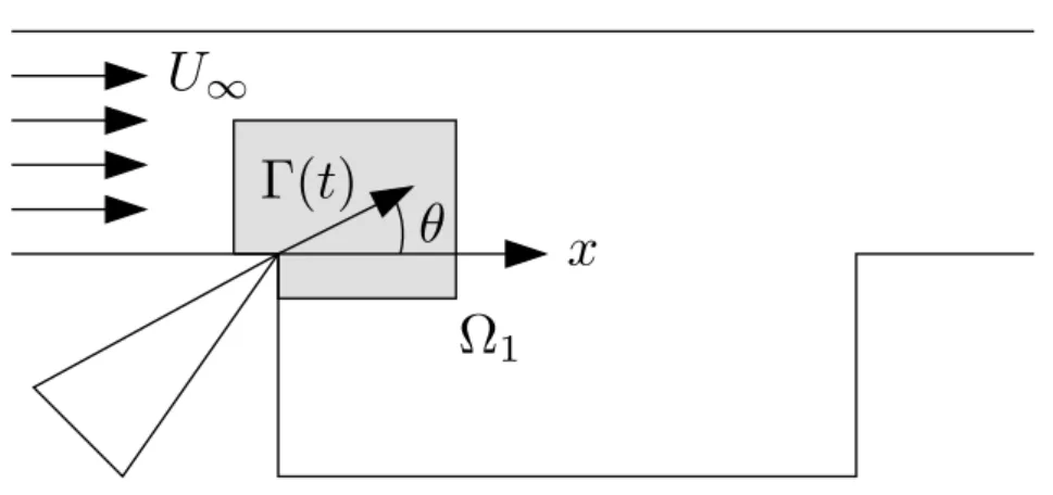
θ
Γ(t)
Ω
1U
∞x
Figure 3. Actuation sub-domain
where αi = (αi1, . . . , αim), and C ∈ Rm×m is the correlation matrix with entries Cij =
hq(·, tj), q(·, ti)iΩ. This method, known as method of snapshots [39], favors spatially-resolved
flow data sets, such as the ones obtained by PIV, over time-resolved data obtained by hot-wire sensor measurements.
3.3. Empirical POD Expansion. To compute the POD basis, a discretization of the domain Ω is employed. Measurements of the flow velocity field u(xi, tj) are acquired using PIV over a grid of points xi ∈ Ω, i = 1, . . . , n at tj, j = 1, . . . , m time instants. In this study, snapshot of
the baseline flow at Mach 0.3 was considered (see Table 1), with n = 16, 384 and m = 1000. The corresponding values of the local speed of sound c(xi, tj) are computed from the local
temperature T (xi, tj) using the relation c = (γRT )1/2, whereas the local temperature is obtained
again from the flow velocity, noticing that for isentropic flows
cpT0 = cpT (x, t) + ku(x, t)k 2
2
where cp is the specific heat at constant pressure and T0 is the measured stagnation temperature. The average ¯q(xi) = m1
Pm
j=1q(xi, tj) is removed from the data, and the POD modes {φk(x)}Nk=1
of the ensemble ˜
q(xi, tj) = q(xi, tj) − ¯q(xi) , i = 1, . . . , n, j = 1, . . . , m
are obtained using the method of snapshots, where numerical integration over the grid replaces the inner product on H for the computation of the correlation matrix C. This yields the empirical POD expansion of the flow variable q(·, ·) as
ˆ qN(x, t) = ¯q(x) + N X k=1 ak(t)φk(x) (3)
computed at the grid points xi, i = 1, . . . , n, where ak(t) = h˜q(·, t), φk(·)iΩ.
3.4. Galerkin Projection and Control Separation. The second step in the process of de-riving a reduced-order model is the projection of the governing equations onto the linear variety
V = ¯q + S, where S is the subspace spanned by the empirical POD modes. The result of this
procedure is a set of nonlinear ODEs describing the dynamics of the coefficients ak(t) in (3).
Writing the governing equations (2) as the functional differential equation (FDE)
˙q = F (q) (4)
where F : H → T H is a vector field on H, the Galerkin projection onto V assigns to (4) the dynamical system
evolving on V. Applying the projection theorem, one obtains
h ˙ˆqN, φkiΩ= hF (ˆqN), φkiΩ, k = 1, . . . , N (6)
and thus, exploiting orthonormality of the POD modes, the FDE (5) can be expressed as the set of ODEs
˙ak(t) = hF (ˆqN(·, t)), φk(·)iΩ, k = 1, . . . , N. (7)
At this stage, the effect of actuation is still buried in the boundary conditions of (2), and does not appear explicitly in (7). The method for separating the effect of actuation from the boundary condition adopted in this study is based on the spatial sub-domain separation idea of [14]. The approach is to identify an actuation domain Ω1 around the exit slot of the actuator, where the
flow is directly affected by the jet velocity. Then, the domain is partitioned into the union of Ω1 and Ω2 = Ω \ Ω1, and the inner product computed separately over the two domains as
< · , · >Ω= < · , · >Ω1 + < · , · >Ω2 . (8) Denoting by Γ(t) the non-dimentionalized magnitude of the actuator jet velocity at the exit slot, and by θ the fixed angle that the jet velocity forms with the longitudinal direction (see Fig. 3), the method proceeds by assuming that
u(x, t) = (Γ(t) cos θ , Γ(t) sin θ) ∀x ∈ Ω1.
Imposing the further condition that u(x, t) satisfies the POD expansion over Ω1 yields ak(t)φk(x) = Γ(t) cos θΓ(t) sin θ c(x, t) − ¯q(x) −XN i6=k ai(t)φi(x) (9)
for all x ∈ Ω1. Using both (8) and (9) in (6) yields a new system of ODEs of the form
˙ak(t) = dk+ N X i=1 lkiai(t) + N X i=1 N X j=1 qkijai(t)aj(t) + [ bk+ N X i=1 hkiai(t) ]Γ(t) , k = 1, . . . , N
which is quadratic in the state variables ak and affine in the control input Γ. Finally, shifting
the origin of the coordinate system to the point a0 ∈ RN solution of the algebraic equation
dk+ N X i=1 lkia0i + N X i=1 N X j=1 qkija0ia0j = 0 ,
one obtains the reduced-order model
˙a = f (a) + g(a)Γ (10)
with state vector a ∈ RN; here, for the sake of simplicity, the same notation a = (a
1, . . . , aN)
has been adopted for the shifted coordinates. Note that the drift and the control vector fields of (10) can be written as
f (a) = F a + ϕ(a) , ϕ(a) = O(kak2)
g(a) = G + γ(a) , γ(a) = O(kak) .
where F = [∂f /∂a](0) is the Jacobian matrix of f (·) at the origin, and G = g(0). Obviously, (10) has an equilibrium at the origin when Γ = 0.
3.5. Stochastic Estimation. The Galerkin system (10) provides a reduced-order state space model of the cavity flow dynamics, suitable for controller design. However, direct measurements of the state a(t) are not available. For experimental implementation of the controller, a state estimate must be obtained from flow variables that can be measured in real-time. PIV data are not suitable for this task, as they are acquired at a slow sampling rate. In any realistic setting, real-time experimental data can only be obtained via surface measurements, e.g. surface pressure or surface shear stress measurements. In the current work, a stochastic estimation method was employed to estimate the state a(t) from measurements of the surface pressure fluctuation
p (x, t). Stochastic estimation was originally proposed by Adrian [2] as a technique to estimate
flow variables at any point of a spatial domain by using statistical information about the flow at a limited number of locations.
Assuming that real-time pressure measurements are available at ` ≥ N distinct locations, a quadratic prediction model can be constructed as
ˆak(t) = ` X i=1 Ckip (xi, t) + ` X i=1 Dkip2(xi, t) + ` X i,j=1 i6=j Dkijp (xi, t)p (xj, t) , k = 1, ..., N. (11) The coefficients of (11) are computed off-line by minimizing the average mean square of the prediction error between the values of ak(tj), available from the snapshots, and the estimated
ones ˆak(tj), i.e., by minimizing the functional
Je= 1 m m X j=1 kˆa(tj) − a(tj)k2.
Since the number of snapshots is usually much larger than the number of the parameters of the prediction model, and the latter is linear in the parameters, the values of Cki and Dkij are readily obtained by solving the over-determined linear systems
∂Je ∂Cki = 0 , ∂Je ∂Dki = 0, ∂Je ∂Dkij = 0, i, j = 1, ..., `
for each k = 1, . . . , N . Similarly, in case ` < N , stochastic estimation can be used to endow the reduced-order model (10) with an output equation of the form
p = h(a)
where p =¡p (x1, ·), . . . , p (x`, ·)
¢
, and the read-out map is given by
hk(a) = ` X i=1 ¯ Ckiai+ ` X i=1 ¯ Dkia2i + ` X i,j=1 i6=j ¯ Dkijaiaj, k = 1, ..., `.
This representation is useful when the order of the model exceeds the number of independent measured outputs, and thus a dynamic observer is required to obtain estimates of the state of the Galerkin model.
4. Feedback Control Design
In this section, the design of a feedback controller based on the model derived in Section 3 is presented and discussed from a mathematical perspective. A single-resonance mode flow at Mach number M = 0.3 (see Table 1) has been selected as a baseline case for the development of the reduced-order model. The uncontrolled flow at Mach 0.3 exhibits a single strong resonant
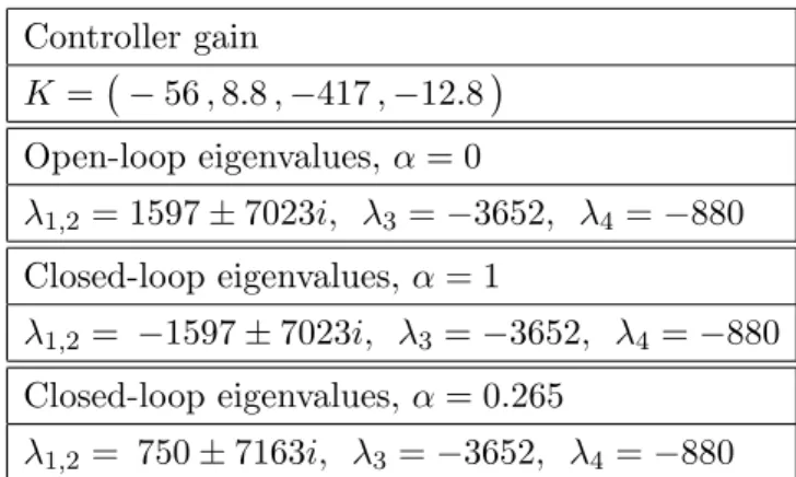
Table 2. Parameters of the Linearized Model Controller gain K =¡− 56 , 8.8 , −417 , −12.8¢ Open-loop eigenvalues, α = 0 λ1,2= 1597 ± 7023i, λ3= −3652, λ4 = −880 Closed-loop eigenvalues, α = 1 λ1,2= −1597 ± 7023i, λ3 = −3652, λ4 = −880 Closed-loop eigenvalues, α = 0.265 λ1,2= 750 ± 7163i, λ3 = −3652, λ4= −880
tone at approximately 2900 Hz, which is very near the frequency of the third Rossiter mode. It has been shown from open-loop experiments that the actuator has sufficient authority to significantly alter the flow at this Mach number (see [12]). The voltage input to the actuator is computed from the commanded non-dimensionalized jet velocity Γ, which is the control input to the reduced-order model (10), by inverting the approximate linear relation Γ = ¯KaVa, where
¯
Ka= Ka/U∞. It is important to point out that, to prevent damaging the actuator, the control
input signal must be limited to the range ±10V . The presence of the saturation plays an important role in the design of the control law, as discussed in the sequel.
The order of the model (10) has been chosen as N = 4, to achieve a tradeoff between accuracy and simplicity of the model for control design. Previous studies [23] have shown that the first 4 POD modes are sufficient to reconstruct the dominant coherent structures. The state vector is estimated using the quadratic prediction model (11) from ` = 6 real-time pressure measurements taken at the locations shown in Fig. 2. The value of the equilibrium point a0 of (10) has been computed numerically using a Newton-like iterative method. Since the solution of the algebraic equation is not unique, and the outcome of the steepest descent search depends on the initial condition, Runge-Kutta simulations of the system (10) with Γ = 0 have been used to discard unfeasible solutions.
The linear approximation of (10) at the origin is readily obtained as
˙a = F a + GΓ , (12)
where the pair (F, G) is controllable. The matrix F possesses two complex conjugate eigenvalues in Re[λ] > 0 and two real eigenvalues in Re[λ] < 0, as shown in Table 2. The presence of two complex conjugate eigenvalues implies, as expected, that the equilibrium a0 is an unstable
solution for the Galerkin model (10). Furthermore, numerical simulations of (10) reveal the existence of a stable limit cycle, consistent with the existence of an unstable manifold at the origin. The frequency of the quasi-steady oscillation for the model is comparable with the dominant tone measured in the cavity in open-loop experiments, suggesting that the reduced-order model is in some agreement with the behavior of the plant.
4.1. Scaled LQ Control. To suppress the oscillation in the cavity, a viable strategy to pursue is the design of a controller that stabilizes the origin of (10), at least locally. Since the reduced-order model is linearly controllable, a simple way of achieving this goal is to select a state-feedback matrix K ∈ R1×4 such that F + GK is Hurwitz, and, by resorting to the principle of
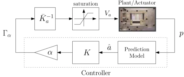
certainty-equivalence, implementing the control law from the estimated state Γ = Kˆa .
Plant/Actuator
Prediction
Model
K
α
ˆa
p
Γ
α
¯
K
−1
a
Controller
saturation
V
aFigure 4. Block diagram of the closed-loop system
Unfortunately, this approach becomes ineffective whenever the limit cycle lies outside the local domain of attraction achieved by the saturated control
Va= sat( ¯Ka−1Kˆa) (13)
which may be much smaller than the one attainable with the unconstrained control. As a matter of fact, experimental results have shown that controllers of the form (13) implemented with a stabilizing gain K result in constant saturation of the control signal, irrespective of the way K is chosen. As it has also been remarked in [33], stabilizing control strategies tend to be unnec-essarily aggressive, requiring large control efforts, and possibly driving the closed loop system outside the limits of validity of the reduced-order model. To remedy this situation, asymptotic stabilization of the origin (which amounts in suppressing the limit cycle) has been traded for the less ambitious goal of attenuating as much as possible the amplitude of the oscillation in steady state. As it will become clear in the sequel, this goal can be easily accomplished by modifying the parameter of the Hopf bifurcation exhibited by the model (10). To this end, the commanded jet velocity has been re-scaled by a factor 0 < α < 1 as follows
Γα = −αKˆa , (14)
where the value of the scaling factor must be tuned experimentally to the largest value such that Γα(t) remains within the actuator constraints. The diagram of the overall closed-loop system
resulting from the implementation of the scaled controller is given in Fig. 4.
Obviously, setting α = 1 results in asymptotic stabilization of the origin, while for α = 0 the system evolves in open-loop; therefore, the closed-loop eigenvalues cross the imaginary axis at a particular value α?. From the point of view of the design, and the subsequent analysis, it is
convenient to select K in such away that α? = 0.5. This can be accomplished by computing
K as the solution of a linear-quadratic regulator problem, with the relative weight between
the penalty on the control and the penalty on the state selected large enough such that the eigenvalues of F + GK mirror those of the open-loop matrix F with respect to the imaginary axis. Specifically, K is obtained by minimizing the cost function
Jc(Γ) = Z ∞
0
£
a(t)Waa(t) + WΓΓ(t)2¤dt
subject to (12), where the positive definite weighting functions for the state vector and the control signal are chosen respectively as
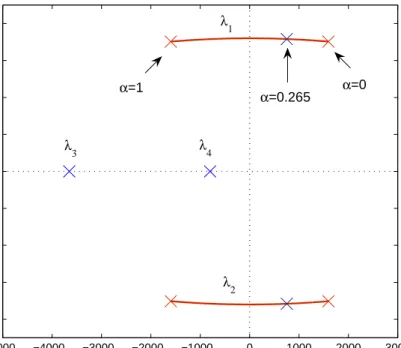
The resulting gain K and the corresponding eigenvalues of the closed-loop system are given in Table 2. Figure 5 shows the location of the eigenvalues of F + αGK in the complex plane for 0 ≤ α ≤ 1. As α increases, the right-half plane eigenvalues migrate to the left half plane, with crossing occurring at α? = 0.5, while the left-half plane open-loop eigenvalues are left unchanged.
Note also that the imaginary part of the complex conjugate eigenvalues is virtually unaffected by the control.
Results of nonlinear simulations of the closed-loop system (10)-(14) show that the amplitude of the limit cycle is attenuated when α increases from 0 to 0.5, whereas the trajectory a(t) converges to the origin when α > 0.5. This indicates that, at least in principle, the scaled LQ controller designed for the linear approximation succeeds in controlling the limit cycle of the low-dimensional nonlinear Galerkin model (10). Experimental results, which will be discussed in detail in Section 5, validate the outcome of the simulations on the finite-dimensional model, and the subsequent analysis. In experiments, the value α = 0.265 was ultimately selected to obtain a control signal within the saturation limits. This choice yields the closed-loop eigenvalues given in Table 2 (see also Fig. 5).
Remark 4.1. It is worth noting that, since F has a pair of eigenvalues in Re[λ] > 0, the optimal
gain K is non-vanishing as the ratio between the penalty on the control and the magnitude of the penalty on the state increases [41]. As a matter of fact, keeping Wa fixed and letting WΓ → +∞, the optimal gain converges to a finite limit K∞ 6= 0. As the given selection of the weights is
such that K ≈ K∞, saturation of the control signal can not be avoided merely by increasing the
penalty on the control energy in the LQ cost function, and the use of the scaling factor α is required.
4.2. Bifurcation Analysis. In what follows, a simple analysis carried out on the basis of the nonlinear Galerkin model (10) is presented to illustrate the motivation behind the choice of the scaled LQ feedback control. Let T ∈ R4×4 be a nonsingular transformation that converts F into modal form, that is,
T F T−1= µ L1 0 0 L2 ¶ where L1 = µ σ −ω ω σ ¶ , L2 = µ −λ1 0 0 −λ2 ¶ , with σ > 0, ω > 0, and λ1, λ2> 0.
Partitioning the state vector a according to the above decomposition, and assuming that ˆa ≡ a, the closed-loop Galerkin system is written in the new coordinates as
˙η = L1η + M1Γα+ ϕ1(η, ζ) + γ1(η, ζ)Γα ˙ζ = L2ζ + M2Γα+ ϕ2(η, ζ) + γ2(η, ζ)Γα, where µ η ζ ¶ = T a , µ M1 M2 ¶ = T G and ϕi(η, ζ) = O(kηk2, kζk2) , γi(η, ζ) = O(kηk, kζk) , i = 1, 2. Note that the control law Γα = −αKa is expressed in the new coordinates as
Γα = −αK1η − αK2ζ ,
for some matrices K1and K2. Since it has been verified that the feedback gain K does not affect
the location of the stable eigenvalues of the open-loop matrix F , necessarily K2= 0. Therefore,
the closed-loop system can be written as
−5000 −4000 −3000 −2000 −1000 0 1000 2000 3000 −8000 −6000 −4000 −2000 0 2000 4000 6000 8000 Re [λ] Im [ λ ] α=1 α=0 α=0.265 λ3 λ4 λ1 λ2
Figure 5. Eigenvalues of the closed-loop matrix F + αGK. ˙ζ = − αM2K2η + L2ζ + ϕ2(η, ζ) − αγ2(η, ζ)K1η .
An easy computation shows that the eigenvalues of the matrix L1− αM1K1 are given by
λ(L1− αM1K1) = (1 − 2α)σ ± i
p
ω2+ 4ασ2(1 − α) .
Letting µ = 1 − 2α and ¯ω(µ) =pω2+ (1 − µ2)σ2, one obtains (modulo a unitary
transforma-tion) L1− αM1K1= µ µσ −¯ω(µ) ¯ ω(µ) µσ ¶ ,
and thus the spectrum of the closed-loop matrix
L(µ) = Ã L1+µ−12 M1K1 0 µ−1 2 M2K2 L2 !
at µ = 0 splits into a pair of purely imaginary eigenvalues and a pair of negative real eigenvalues. This implies the existence of a center manifold for the trajectories of the Galerkin system. Specifically, let L(µ) = µ L11(µ) 0 L21(µ) L2 ¶ , Φi(η, ζ, µ) = ϕi(η, ζ) − αγi(η, ζ)K1η , i = 1, 2
and write the closed-loop Galerkin system as ˙µ = 0
˙η = L11(µ)η + Φ1(η, ζ, µ)
˙ζ = L21(µ)η + L2ζ + Φ2(η, ζ, µ) , (15)
where
103 104 85 90 95 100 105 110 115 120 125 130 135 M = 0.30 frequency (Hz) SPL (dB) open−loop closed−loop (a) 10 3 104 85 90 95 100 105 110 115 120 125 130 135 M = 0.30 frequency (Hz) SPL (dB) open−loop closed−loop (b) Figure 6. (a)Sound pressure level measured at location #5,
(b) Sound pressure level measured at location #6;
Feedback control experiment at Mach 0.3 (design conditions). Thin line: baseline flow. Thick line: controlled flow (closed-loop).
and a trivial dynamics for the bifurcation parameter µ has been added to the model. The Center Manifold Theorem [7] establishes the existence of an exponentially attracting submanifold of the state space, which is described by the graph of a smooth mapping ζ = π(η, µ) satisfying
π(0, µ) = 0, [∂π/∂η](0, µ) = 0, and ∂π
∂η[L11(µ)η + Φ1(η, π(η, µ), µ)] = L21(µ)η
+L2π(η, µ) + Φ2(η, π(η, µ), µ)
for all (η, µ) in a neighborhood of (0, 0). This allows to reduce the analysis of system (15) to the restriction of its dynamics onto the center manifold, which in the given set of coordinates
reads as µ ˙η1 ˙η2 ¶ = µ µσ −¯ω(µ) ¯ ω(µ) µσ ¶ µ η1 η2 ¶ + µ Φ11(η, π(η, µ), µ) Φ12(η, π(η, µ), µ) ¶ .
A near-identity transformation into Poincar`e normal form [44] yields1 Φ11(η, µ) = ¡ − a(µ)η1− b(µ)η2 ¢¡ η21+ η22¢+ O(kηk5) Φ12(η, µ) = ¡ b(µ)η1− a(µ)η2 ¢¡ η21+ η22¢+ O(kηk5)
where a(·) and b(·) are smooth functions. For the model under investigation, it turns out that
a(µ) > 0 and b(µ) > 0 for all −1 ≤ µ ≤ 1. Finally, using polar coordinates ρ = (η2
1 + η22)1/2, θ = tan−1(η
2/η1), one obtains the system
˙ρ = µσρ − a(µ)ρ3+ O(ρ5)
˙θ = ω + b(µ)ρ2+ O(ρ4) . (16)
The structure of system (16) reveals that the original closed-loop Galerkin system has a locally exponentially stable equilibrium at the origin for µ < 0, and undergoes a Hopf-Poincar`e-Andropov bifurcation at µ = 0, with a stable limit cycle for µ > 0. The amplitude and frequency of the limit cycle are given respectively by
ρ?(µ) = r µσ a(µ), ω ?(µ) = ¯ω(µ) + b(µ) µσ a(µ)
1A similar simplified expression for the reduction of the Galerkin system onto the center manifold can be
from which, since a(µ) = O(1), it is readily seen that the amplitude of the oscillation decreases as µ → 0+. Recalling the definition of µ, the result of the analysis can be summarized as follows:
(1) If it is required to set α < 0.5 to avoid saturating the actuator, the origin of the Galerkin system can not be stabilized at all.
(2) If this is the case, the application of linear feedback can still lower the amplitude of the limit cycle, but only up to a minimum value imposed by the actuator limits.
Notwithstanding the above result, it may still be possible to reduce the amplitude of the cavity tone beyond the limit achievable using linear feedback, resorting to more elaborate control strategies (nonlinear and/or time-varying feedback).
The experimental results discussed in the next section seem to support the analysis, as the controller is capable to attenuate the resonance in the cavity to a certain extent, while complete suppression seems to be unattainable within the limitations imposed by the actuator and the fidelity of the reduced-order model.
5. Experimental Results
The performance of the scaled feedback control law has been tested experimentally in design and off-design conditions, and compared with the results obtained using feed-forward control (specifically the open-loop periodic forcing approach of [12].) The design conditions refer to the Mach 0.3 baseline flow, whose parameters are given in Table 1, used for identification of the reduced-order model. For the scaled LQ controller (14), the value of the scaling parameter was determined experimentally by increasing α in the closed-loop system until the voltage input to the actuator reached the maximum allowable range. The maximum value of α compatible with the actuator limits was found to be equal to 0.256, and thus asymptotic stabilization of the origin of the reduced-order Galerkin model can not be achieved. Nonetheless, the experimental results shown in Fig. 6 indicate that an attenuation of about 15 dB of the sound pressure level at the resonance frequency fr = 2900 Hz (as measured by the pressure sensors at the locations no. 5
and no. 6, Fig. 2) is attained in closed-loop operations. Although, as expected, the results for the two sensors present some differences, in both cases it is noticeable that the controller induces a redistribution of the energy into various modes at frequencies frequencies. This indicates that the dynamics of the flow have been captured by the reduced-order model (and by the static prediction model) to an extent which enables model-based control design.
The robustness of the closed-loop system to variations in the flow conditions has been tested performing experiments with different values of the Mach number selected in the range M ∈ [0.27, 0.32], where the baseline flow still preserves a dominant single-tone characteristic. The results of closed-loop experiments pertaining to the M = 0.27 and M = 0.32 are shown in Fig. 7 and Fig. 8, respectively. In these off-design flow conditions, while the performance deteriorate to some degree, similar benefits and characteristics of the nominal closed-loop system are main-tained. The dominant resonance peak is significantly attenuated, with flow energy being spread into a larger range of frequencies, while noticeable peaks begin to appear at higher frequen-cies for the Mach 0.27 case in Fig. 7 (a) and at lower frequenfrequen-cies for the Mach 0.32 case in Fig. 8 (b), respectively. The closed-loop SPL spectra obtained with the scaled LQ controller re-semble those previously obtained by this group using a proportional control with time delay [48]. Furthermore, the two controllers present similar robustness properties for off-design conditions considered here. The similarities may suggest that, although through different processes, anal-ogous physical mechanisms are activated at the receptivity region of the cavity shear layer in closed-loop operations.
Finally, a comparison has been made with the feed-forward control approach of [12]. Here, periodic open-loop forcing of the flow at frequency fc= 3920 Hz is applied, where the frequency
of the excitation has been chosen experimentally to yield the largest attenuation of the dominant tone at Mach 0.3, which is regarded as the nominal design condition. While in [12] the selection
103 104 85 90 95 100 105 110 115 120 125 130 135 M = 0.27 frequency (Hz) SPL (dB) open−loop closed−loop (a) 10 3 104 85 90 95 100 105 110 115 120 125 130 135 M = 0.27 frequency (Hz) SPL (dB) open−loop closed−loop (b) Figure 7. (a)Sound pressure level measured at location #5,
(b)Sound pressure level measured at location #6;
Feedback control experiment at Mach 0.27 (off-design conditions). Thin line: baseline flow. Thick line: controlled flow (closed-loop).
103 104 85 90 95 100 105 110 115 120 125 130 135 M = 0.32 frequency (Hz) SPL (dB) open−loop closed−loop (a) 10 3 104 85 90 95 100 105 110 115 120 125 130 135 M = 0.32 frequency (Hz) SPL (dB) open−loop closed−loop (b) Figure 8. (a)Sound pressure level measured at location #5, (b)Sound pressure level measured at location #6;
Feedback control experiment at Mach 0.32 (off-design conditions). Thin line: baseline flow. Thick line: controlled flow (closed-loop).
of the frequency of the excitation is updated on line by an extremum-seeking mechanism, in this study the frequency has been kept constant, to allow a fair comparison between open-loop and closed-loop strategies of fixed structure, especially as far as robustness is concerned. The results achieved in design conditions, shown in Fig. 9, reveal that, while the feed-forward strategy outperforms the LQ control as far as the mere attenuation of the resonance peak is concerned, this is accompanied by the introduction of one or two new significant peaks, including (but not limited to) at the forcing frequency itself. In addition, it must be expected that the performance of feed-forward control degrades when operating in off-design conditions. This is confirmed by the results obtained at Mach 0.32, which are shown in Fig. 10: In the worst case, as measured at location no. 6, the periodic forcing induces a new resonance at about the second Rossiter mode, which has even larger magnitude than the original baseline resonance tone. The poor performance exhibited by feed-forward control strategies when operating in different regimes than the nominal flow conditions makes indeed a compelling argument for the applications of feedback control methodologies, as an effective means to account for model uncertainties.
103 104 85 90 95 100 105 110 115 120 125 130 135 frequency (Hz) SPL (dB) Mach 0.30 baseline open−loop forcing (a) 10 3 104 85 90 95 100 105 110 115 120 125 130 135 frequency (Hz) SPL (dB) Mach 0.30 baseline open−loop forcing (b) Figure 9. (a)Sound pressure level measured at location #5, (b)Sound pressure level measured at location #6;
Feed-forward control experiment at Mach 0.3. Thin line: baseline flow. Thick line: controlled flow (open-loop forcing at fc= 3920 Hz).
6. Conclusions
This paper presents the development and the experimental verification of a systematic model-based approach for active flow control, which includes system identification and control design. The benchmark problem tackled in this work is the suppression of a single-mode resonance induced by a subsonic flow over a shallow cavity. Experimental results, in qualitative agreement with the analysis on the reduced-order model, show that the controller achieves a significant attenuation of the target resonance peak, exhibits good robustness for some off-design conditions, and compares favorably with tuned open-loop strategies. Although the experimental setup is the same as the one used in [12] and [48], the modeling, identification, and control design techniques are different, as the reduced-order model considered here is nonlinear, as opposed to the linear one considered in [48]. Furthermore, while the results presented here are similar to those obtained in [48], the analysis performed on the nonlinear model has revealed a fundamental limitation posed by the bounded control authority of the actuator.
Despite being quite encouraging, the results presented here are far from being fully satisfac-tory, and point to much further work ahead. Several important issues remain to be resolved, as the effect of feedback on the flow dynamics is not well understood yet. Further investigation is needed to understand how to incorporate more effectively the presence of actuation in reduced-order flow models. The method for control separation used in this work acts “a posteriori” with respect to the generation of the POD basis, as the separation is performed solely at the level of the Galerkin projection. A more direct approach is currently being investigated, which considers a POD-like expansion of the flow field which includes certain “actuation modes”, determined from experimental data, whose modal coefficients depend directly on the actuation variable. Another important issue, which is too often overlooked, is the influence of the actuator dynam-ics on the overall performance of the closed-loop system. An on-going research effort is being devoted to modeling and identification of dynamics of the synthetic jet-like acoustic actuator employed in the experimental apparatus, and to the design of servo-controller to achieve precise tracking of the commanded jet velocity input. Finally, the use of dynamic observers (as pro-posed in [32]) or dynamic auto-regressive prediction models may constitute a better alternative to static stochastic estimation methods for real-time estimation of the state of the reduced-order models. All these issues are currently being addressed.
103 104 85 90 95 100 105 110 115 120 125 130 135 frequency (Hz) SPL (dB) Mach 0.32 baseline open−loop forcing (a) 10 3 104 85 90 95 100 105 110 115 120 125 130 135 frequency (Hz) SPL (dB) Mach 0.32 baseline open−loop forcing (b) Figure 10. (a)Sound pressure level measured at location #5, (b) Sound pres-sure level meapres-sured at location #6;
Feed-forward control experiment at Mach 0.32. Thin line: baseline flow. Thick line: controlled flow (open-loop forcing at fc= 3920 Hz).
Acknowledgment
The authors would like to thank Louis Cattafesta, Clancy Rowley, Gilead Tadmor and David Williams for fruitful and insightful discussions. The contribution of our colleagues at CCCS, James DeBonis, Chris Camphouse, Kihwan Kim and Co¸sku Kasnako˘glu is gratefully acknowl-edged.
References
[1] Aamo, O. M., and Krstic, M., Flow control by feedback : stabilization and mixing. New york, NY: Springer Verlag, 2003.
[2] Adrian, R. J., “On the role of conditional averages in turbulent theory,” in Turbulence in Liquids. Princeton: Science Press, 1979.
[3] Atwell, J. A., and King, B. B., “Reduced order controllers for spatially distributed systems via proper orthogonal decomposition,” SIAM Journal on Scientific Computing, vol. 26, no. 1, pp. 128–151, 2004. [4] Berkooz, G., Holmes, P., and Lumley, J. L., “The proper orthogonal decomposition in the analysis of turbulent
flows.” Annual Review of Fluid Mechanics, vol. 25, pp. 539–575, 1993.
[5] Caraballo, E., Yuan, X., Little, J., Debiasi, M., Yan, P., Serrani, A., Myatt, J. H., and Samimy, M., “Feedback control of cavity flow using experimental based reduced order model,” in Proceedings of the 35th AIAA Fluid Dynamics Conference and Exhibit, Toronto, ON, 2005, AIAA Paper 2005-5269.
[6] Caraballo, E., Little, J., Debiasi, M., and Samimy, M., “Development and Implementation of an Experimental Based Reduced-order Model for Feedback Control of Subsonic Cavity Flows,” Journal of Fluids Engineering, Vol. 129, No. 7, pp. 813-824, July 2007.
[7] Carr, J., Applications of Centre Manifold Theory. Springer Verlag, 1981.
[8] Cattafesta, L. N., Garg, S., Kegerise, M. S., and Jones, G. S., “Experiments on compressible flow-induced cavity oscillations,” in Proceedings of the 29th Fluid Dynamics Conference, Albuquerque, NM, 1998, AIAA Paper 1998-2912.
[9] Cattafesta, L., Williams, D., Rowley, C., and Alvi, F., “Review of active control of flow-induced cavity resonance,” in Proceedings of the 33rd AIAA Fluid Dynamics Conference and Exhibit, Orlando, FL, 2003, AIAA Paper 2003-3567.
[10] Chorin, A., and Marsden, J., A mathematical introduction to fluid mechnanics, 3rd ed. Springer-Verlag,
1993.
[11] Cohen, K., Siegel, S., and McLaughlin, T., “Proper orthogonal decomposition modeling of a controlled Ginzburg-Landau cylinder wake model,” in Proceedings of the 41st AIAA Aerospace Sciences Meeting and Exhibit, Reno, NV, 2003, AIAA Paper 2003-1292.
[12] Debiasi, M., and Samimy, M., “Logic-based active control of subsonic cavity flow resonance,” AIAA Journal, vol. 42, no. 9, pp. 1901–1909, 2004.
[13] Delville, J., Cordier, L., and Bonnet, J., “Large-scale-structure identification and control in turbulent shear
flows,” in Flow Control: Fundamentals and Practice, P. A. Gad-el Hak, M. and J. Bonnet, Eds.
[14] Efe, M., and ¨Ozbay, H., “Low dimensional modelling and Dirichlet boundary controller design for Burgers equation,” International Journal of Control, vol. 77, no. 10, pp. 895–906, 2004.
[15] Fitzpatrick, K., Feng, Y., Lind, R., Kurdila, A. J., and Mikolaitis, D. W., “Flow control in a driven cavity incorporating excitation phase differential,” Journal of Guidance, Control, and Dynamics, vol. 28, no. 1, pp. 63–70, January 2005.
[16] Gad-el Hak, M., Pollard, A., and Bonnet, J. P., Eds., Flow control: Fundamentals and practices. Berlin,
Germany: Springer-Verlag, 1998.
[17] Gad-el Hak, M., Flow Control: Passive, Active, and Reactive Flow Management. New York, NY: Cambridge University Press, 2000.
[18] Gharib, M., “Response on the cavity shear layer oscillations to external forcing,” AIAA Journal, vol. 25, no. 1, pp. 43–7, 1987.
[19] Glauser, M., Higuchi, H., Ausseur, J., and Pinier, J., “Feedback control of separated flows,” in Proceedings of the 2nd AIAA Flow Control Conference, Portland, OR, 2004.
[20] Heller, H. H., and Bliss, D. B., “The physical mechanisms of flow-induced pressure fluctuations in cavities and concepts for their suppression,” in Proceedings of the 2nd AIAA Aero-Acoustics Conference, Hampton, VA, 1975, AIAA Paper 75-491.
[21] Holmes, P., Lumley, J., and Berkooz, G., Turbulence, Coherent Structures, Dynamical System, and Symmetry. Cambridge: Cambridge University Press, 1996.
[22] Kegerise, M. A., Spina, E. F., Garg, S., and Cattafesta, L. N., “Mode-switching and nonlinear effects in compressible flow over a cavity,” Physics of Fluids, vol. 16, no. 3, pp. 678–687, 2004.
[23] Little, J., Debiasi, M., and Samimy, M., “Effects of Open-loop and Closed-loop Control on Subsonic Cavity Flows, Physics of Fluids, Vol. 19, No. 6, 2007.
[24] Lumley, J., “The structure of inhomogeneous turbulent flows,” Atmospheric Turbulence and Radio Wave Propagation, pp. 166–178, 1967.
[25] Noack, B. R., Afanasiev, K., Morzynski, M., Tadmor, G., and Thiele, F., “A hierarchy of low-dimensional models for the transient and post-transient cylinder wake,” Journal of Fluid Mechanics, vol. 497, pp. 335–63, 2003.
[26] Noack, B., Tadmor, G., and Morzynski, M., “Actuation models and dissipative control in empirical Galerkin models of fluid flows,” in Proceedings of the 2004 American Control Conference, Boston, MA, 2004. [27] Rediniotis, O. K., Ko, J., and Kurdila, A. J., “Reduced order nonlinear Navier-Stokes models for synthetic
jets,” Transactions of the ASME. Journal of Fluids Engineering, vol. 124, no. 2, pp. 433–443, 2002. [28] Rockwell, D., and Naudascher, E., “Review of self-sustaining oscillations of flow past cavities,” Transactions
of the ASME. Journal of Fluids Engineering, vol. 100, no. 2, pp. 152–65, 1978.
[29] Rossiter, J., “Wind tunnel experiments on the flow over rectangular cavities at subsonic and transonic speeds,” RAE Tech. Rep. 64037, and Aeronautical Research Council Reports and Memoranda No. 3438, Tech. Rep., 1964.
[30] Rowley, C. W., Colonius, T., and Basu, A. J., “On self-sustained oscillations in two-dimensional compressible flow over rectangular cavities,” Journal of Fluid Mechanics, vol. 455, pp. 315–346, 2002.
[31] Rowley, C. W., Colonius, T., and Murray, R. M., “Model reduction for compressible flows using POD and Galerkin projection,” Physica D, vol. 189, no. 1-2, pp. 115–29, 2004.
[32] Rowley, C., and Juttijudata, V., “Model-based control and estimation of cavity flow oscillations,” in Pro-ceedings of the 44th IEEE Conference on Decision and Control, Seville, Spain, 2005.
[33] Rowley, C., and Williams, D., “Dynamics and control of high-reynolds-number flow over open cavities,” Annual Review of Fluid Mechanics, vol. 38, no. 1, pp. 251–276, 2006.
[34] Rowley, C., Williams, D., Colonius, T., Murray, R., MacMartin, D., and Fabris, D., “Model-based control of cavity oscillations, part II: System identification and analysis,” in Proceedings of the 40th AIAA Aerospace Sciences Meeting, Reno, NV, 2002, AIAA Paper 2002-0972.
[35] Rowley, C. W., Williams, D. R., Colonius, T., Murray, R. M., and MacMynowski, D. G., “Linear models for control of cavity flow oscillations,” Journal of Fluid Mechanics, vol. 547, pp. 317–330, 2006.
[36] Sahoo, D., Annaswamy, A., Zhuang, N., and Alvi, F., “Control of cavity tones in supersonic flow,” in Proceedings of the 43rd AIAA Aerospace Sciences Meeting and Exhibit, Reno, NV, 2005, AIAA Paper 2005-793.
[37] Samimy, M., Debiasi, M., Caraballo, E., Serrani, A., Yuan, X., Little, J., and Myatt, J. H., “Feedback Control of Subsonic Cavity Flows Using Reduced-order Models,” Journal of Fluid Mechanics, 579, pp. 315-346, May 2007.
[38] Singh, S. N., Myatt, J. H., Addington, G. A., Banda, S., and Hall, J. K., “Optimal feedback control of vortex shedding using proper orthogonal decomposition models,” Transactions of the ASME. Journal of Fluids Engineering, vol. 123, no. 3, pp. 612–618, 2001.
[39] Sirovich, L., “Turbulence and the dynamics of coherent structures,” Quarterly of Applied Math., vol. XLV, no. 3, pp. 561–590, 1987.
[40] Staneck, M., Raman, G., Kibens, V., Ross, J., Odedra, J., and Peto, J., “Control of cavity resonance through very high frequency forcing,” in Proceedings of the 21st AIAA Aeroacoustics Conference, Lahaina, HI, 2000, AIAA Paper 2000-1905.
[41] Stengel, R., Optimal Control and Estimation. New York, NY: Dover, 1994.
[42] Tadmor, G., Noack, B., Dillmann, A., Gerhard, J., Pastoor, M., King, R., and Morzynski, M., “Control, observation and energy regulation of wake flow instabilities,” in Proceedings of the 42nd IEEE Conference on Decision and Control, Maui, HI, 2003.
[43] Tilmann, C. P., Kimmel, R. L., Addington, G. A., and Myatt, J. H., “Flow control research and applications at the AFRL’s Air Vehicles Directorate,” in Proceedings of the 2nd AIAA Flow Control Conference, Portland, OR, 2004, AIAA Paper 2004-2611.
[44] Wiggins, S., Introduction to applied nonlinear dynamical systems and chaos, 2nd ed. New York, NY:
Springer-Verlag, 2003.
[45] Williams, D. R., Fabris, D., and Morrow, J., “Experiments on controlling multiple acoustic modes in cavities,” in Proceedings of the 21st AIAA Aeroacoustics Conference, Lahaina, HI, 2000, AIAA Paper 2000-1903. [46] Williams, D., and Rowley, C., “Recent progress in closed-loop control of cavity tones,” in Proceedings of the
44th AIAA Aerospace Sciences Meeting, Reno, NV, 2006, AIAA Paper 2006-0712.
[47] Williams, D. R., Rowley, C., Colonius, T., Murray, R., MacMartin, D., Fabris, D., and Albertson, J., “Model-based control of cavity oscillations part I: Experiments,” in Proceedings of the 40th AIAA Aerospace Sciences Meeting, 2002, AIAA Paper 2002-0971.
[48] Yan, P., Debiasi, M., Yuan, X., Little, J., ¨Ozbay, H., and Samimy, M., “Experimental study of linear
closed-loop control of subsonic cavity flow,” AIAA Journal, vol. 44, no. 5, pp. 929–938, 2006.
Xin Yuan - received the B. E. degree in Control Engi-neering and the M. E. degree in Astronautics from Harbin Institute of Technology, Harbin, China, in 1999 and 2001 respective, and the Ph.D. degree in Electrical Engineer-ing from The Ohio State University in 2006. In 2008, Dr. Yuan joined International Truck and Engine Corpo-ration, Melrose Park, IL, where she is currently a project engineer in advanced controls department.
Her current research interests are dynamic system modeling and control system design, and application to engine controls. Dr. Yuan has authored or coauthored more than 20 technical papers.
Dr. Edgar Caraballo - is a Visiting Scholar at the Gas Dynamics and Turbulence Laboratory (GDTL) of Ohio State University. His areas of research expertise include Reduced Order Modeling and its use in flow control ap-plications, as well as experimental studies of shock wave boundary layer interaction and control in supersonic inlet flows.
He received his PhD in Mechanical Engineering (2008) and MS degree in Mechanical Engineering (2001) from The Ohio State University, and his BS degree in Mechanical Engineering (1993) from the University of Carabobo. He was an Associate Professor in the Department of Mechanical Engineering of the University of Carabobo in the Thermal/Fluid Sciences area from 1993 until 2003.
Jesse Little - is a Ph.D. Candidate in Mechanical En-gineering at The Ohio State University (OSU). He is a member of the Gas Dynamics and Turbulence Labora-tory at OSU and has research expertise in experimental fluid mechanics. His dissertation topic is control of flow separation using plasma actuators. He earned B.S. and M.S. degrees in Mechanical Engineering at OSU in 2004 and 2005 focusing on the study of subsonic cavity flows.
Marco Debiasi - received a B.S. in Mechanical En-gineering in 1995 from the University of Padova, Italy. In 1994-95 he qualified to serve as a Second Lieutenant of the Aeronautica Militare (Italian Air Force). Subse-quently, he obtained a M.S. (1998) and a Ph.D. (2000) in Mechanical and Aerospace Engineering from the Uni-versity of California, Irvine, USA. From 2001 he super-vised the experimental activities of the closed-loop flow control team of the Gas Dynamics and Turbulence Labo-ratory of The Ohio State University, Columbus, USA. In 2006 he joined the Temasek Laboratories of the National University of Singapore where he leads the Experimental Aeroscience Group.
Andrea Serrani - received the B.Eng. (Laurea) de-gree cum laude in Electrical Engineering from the Uni-versity of Ancona, Italy, in 1993, and the Ph.D. degree (Dottorato di Ricerca) in Artificial Intelligence Systems from the same institution in 1997. From 1994 to 1999, he was a Fulbright Fellow at Washington University in St.Louis, where he obtained the M.S. and the D.Sc. de-grees in Systems Science and Mathematics in 1996 and 2000. Since 2002, he has been with the Department of Electrical and Computer Engineering at The Ohio State University, Columbus, Ohio, where he is currently an As-sociate Professor.
His research activity lies in the field of control and systems theory, with emphasis on nonlinear control, tracking and regulation, and application to aerospace and marine systems. His latest research interests include modeling and control of air-breathing hypersonic vehicles, time-varying systems, and experimentally-based aerodynamic flow control. He is the coauthor (with A. Isidori and L. Marconi) of the book Robust Autonomous Guidance -An Internal Model Approach, published by Springer Verlag. Prof. Serrani is an Associate Editor for Automatica, the International Journal of Robust and Nonlinear Control, and the IEEE CSS Conference Editorial Board.
James Myatt - earned a Bachelor of Aerospace Engi-neering from the Georgia Institute of Technology in 1988. He then received a Master of Science in Aerospace Engi-neering from Texas AM University in 1991 and a Ph.D. in Aeronautics Astronautics from Stanford University in 1997. James is a senior aerospace engineer at the Air Force Research Laboratory’s Air Vehicles Directorate, Wright-Patterson AFB, OH, and an Associate Fellow of the American Institute of Aeronautics Astronautics.
Professor Mo Samimy -is the Howard Winbigler
Professor of Engineering at the Ohio State University and Director of Gas Dynamics and Turbulence Labora-tory. He received his B.S. degree in mechanical engineer-ing from Sharif University of Technology in Tehran and M.S. and Ph.D. degrees from the University of Illinois in Urbana-Champaign. His research interests are flow control, compressible turbulence, aeroacoustics, and ex-perimental techniques. He has published extensively on these topics. Prof. Samimy has served in various national committees and editorial boards and lectured extensively in the U.S. and abroad. He is a fellow of the American Society of Mechanical Engineers and the American Insti-tute of Aeronautics and Astronautics.