An Algorithm for Automated Layout of Process
Description Maps Drawn in SBGN
Begum Genc
1,2
and Ugur Dogrusoz
2,3∗
1
The Insight Centre for Data Analytics, University College Cork, Western Road, Cork, Ireland
2
Computer Eng. Dept., Faculty of Eng., Bilkent Univ., Rectorate Building, Ankara 06800, Turkey
3
Sander Lab, Memorial Sloan-Kettering Cancer Center, 417 E68th St., NY 10065, New York, USA
ABSTRACT
Motivation: Evolving technology has increased the focus on genomics. The combination of today’s advanced techniques with decades of molecular biology research have yielded huge amounts of pathway data. A standard, named the Systems Biology Graphical Notation (SBGN), was recently introduced to allow scientists
to represent biological pathways in an unambiguous,
easy-to-understand, and efficient manner. Although there are a number of automated layout algorithms for various types of biological networks, currently none specialize on process description maps as defined by SBGN.
Results: We propose a new automated layout algorithm for process
description maps drawn in SBGN. Our algorithm is based on a force-directed automated layout algorithm called Compound Spring Embedder (CoSE). On top of the existing force scheme, additional heuristics employing new types of forces and movement rules are defined to address SBGN-specific rules. Our algorithm is the only automatic layout algorithm that properly addresses all SBGN rules for drawing process description maps, including placement of substrates and products of process nodes on opposite sides, compact tiling of members of molecular complexes, and extensively making use of nested structures (compound nodes) to properly draw cellular locations and molecular complex structures. As demonstrated experimentally, the algorithm results in significant improvements over use of a generic layout algorithm such as CoSE in addressing SBGN rules on top of commonly accepted graph drawing criteria.
Availability: An implementation of our algorithm in Java is available
within ChiLay library (https://github.com/iVis-at-Bilkent/chilay).
Contact: [email protected]
Supplementary information: Supplementary document is available
at Bioinformatics online.
1
INTRODUCTION
Popular belief is that diagrams directly address people’s innate
cognitive abilities (Larkin and Simon, 1987). Due to the fact that
symbols, diagrams, and other graphical representations vary widely
around the world, it is necessary to have a common interpretation.
Standard notations play an important role in communication and
facilitate rapid development in many research areas.
∗to whom correspondence should be addressed
To address this issue in the field of systems biology,
a
group of modellers, biochemists and software engineers published
the Systems Biology Graphical Notation (SBGN), which allows
scientists to represent biological pathways and networks in an
easy-to-understand and efficient way (Le Nov`ere et al., 2009). It
consists of three complementary languages: process descriptions
(PD), activity flows (AF) and entity relationships (ER).
In this paper, we propose a new automated layout algorithm that
enforces SBGN-specific rules for PD maps. As depicted in Figure 1,
layouts produced by general purpose graph layout algorithms fall
short in certain significant ways:
i. Product and substrate edges of a process node are not
necessarily placed on opposite sides of associated process
nodes. Moreover, SBGN states that each process has two ports
as attachment points,
ii. Degree zero members inside a molecular complex are not
efficiently packed, often wasting large amounts of area,
iii. Cellular locations of processes are not shown in the map.
Our proposed layout algorithm is the only one that successfully
addresses these issues, producing layouts that comply with
SBGN-PD notation. Other software providing SBGN-SBGN-PD maps make use of
generic layout algorithms with limited success. For instance, Vanted
(Junker et al., 2006) provides generic force directed layout with no
support for compound structures. CellDesigner (Funahashi et al.,
2003) also provides a rich set of generic layout algorithms, including
one with compound support imported from a commercial library.
2
BACKGROUND
2.1
Graphs and process description maps
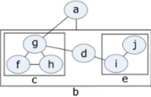
The basics of graph theory are provided in the Supplementary document. A compound graph (Figure 2) C = (V, E, F ) consists of nodes V , adjacency edges E, and inclusion edges F (Dogrusoz et al., 2009).
An SBGN-PD map represents all the molecular processes and interactions taking place between biochemical entities, and their results. The underlying representation is essentially a bipartite compound graph. These maps depict how entities or so called entity pool nodes (EPN) transition from one form to another as a result of different influences, portraying the temporal qualities of molecular events occurring in biochemical reactions (Le Nov`ere et al.,
1
Associate Editor: Prof. Alfonso Valencia
© The Author(s) 2015. Published by Oxford University Press.
This is an Open Access article distributed under the terms of the Creative Commons Attribution License
Bioinformatics Advance Access published September 10, 2015
at Bilkent University on December 18, 2015
http://bioinformatics.oxfordjournals.org/
Fig. 1. SBGN states that product and substrate edges of a process node (small gray squares) should be placed on opposite sides of the associated process node, attached via an input and an output port, respectively (A). A general purpose layout algorithm will not properly pack degree zero members (rounded rectangles with information bulbs) inside a molecular complex (B). The processes that take place inside a cellular compartment are not clearly separated from those occurring outside that compartment (C).
Fig. 2. An example compound graph of multiple levels of nesting, where V = {a, b, . . . , j}, E = {{a, b}, {a, g}, {d, e}, {d, g}, {f, g}, {f, h}, {g, h}, {i, j}}, and F = {bc, bd, be, cf, cg, ch, ei, ej}.
2009). The way in which one type of entity is transformed into another is conveyed by a process node. We call EPN’s consumed and produced by a process substrate (input) and product (output) nodes, respectively. In addition, the EPNs that control (e.g., modulate or stimulate) a process are called effector nodes (Figure 3).
An exchange file format for SBGN maps named SBGN-ML was recently introduced (van Iersel et al., 2012).
2.2
Automated layout and CoSE
The purpose of performing layout on a graph is to make a pictorial representation that is as clear and pleasant as possible. A poor layout of a graph may confuse the user, whereas a well organized and aesthetically pleasing layout can improve the user’s ability to understand the underlying data. Criteria of a good layout may differ from person to person. However, among the generally accepted ones (Battista et al., 1998) are minimal total drawing area, number of edge-edge crossings, and total edge length, producing uniform edge lengths, and ability to reflect any symmetries in the network.
Force-directed layout algorithms (also known as spring embedders) are arguably the most popular type of automatic graph layout, where the basic idea is to simulate a physical system obeying the laws of Hooke and Coulomb.
Fig. 3. A sample process node with three subtsrate nodes and two product nodes, and two effector (one modulator and one stimulator) nodes
Compound Spring Embedder (CoSE) is a force-directed layout algorithm that supports compound nodes (Dogrusoz et al., 2009). Certain additions have been made on the basic spring embedder model to handle compound nodes. The main idea is to represent an expanded node and its associated nested graph as a single entity, similar to a “cart”, which can move freely (details provided in the Supplementary document).
2.3
Rectangle packing and compaction
The rectangle packing problem can be defined as packing a number of non-uniformly sized, rectangle shaped objects into a container, such that there will be no overlaps between the objects and the container will be as compact as possible. This problem, defined in two-dimensions, is an NP-hard problem (Garey and Johnson, 1979).
Almost all graph drawing algorithms try to minimize drawing area by assuming that the graph is connected (Dogrusoz et al., 2002). However, if the graphs have disconnected members (e.g., members of molecular complexes), most such algorithms yield poor results in respect to minimizing wasted area. Various packing techniques have been used in graph layout to pack disconnected parts (disconnected nodes or connected components) of a graph, including tiling (Dogrusoz, 2002) and polyomino packing (Freivalds et al., 2001). Success of a packing method is usually measured by the
adjusted fullnessof the resulting drawing, which is basically the ratio of
the total area of the nodes being packed to the area of the tightest bounding rectangle with specified aspect ratio for the drawing.
at Bilkent University on December 18, 2015
http://bioinformatics.oxfordjournals.org/
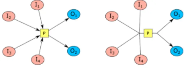
Fig. 4. Drawing of processes in CoSE (left) vs. SBGN (right); SBGN makes use of ports to clearly separate what is consumed and produced by a process.
Results of packing could often be improved through computation of a visibility graph and applying compaction (de Berg et al., 2008). The visibility in this context refers to the feasibility of drawing a collision-free straight line between two nodes.
3
METHODS
We introduce a new, specialized algorithm for layout of SBGN-PD maps. Since SBGN-PD notation makes exclusive use of compound structures, our algorithm was based on CoSE, addressing SBGN specific rules in process description maps as summarized here and detailed subsequently:
i. Additional force types and associated procedures on top of the force scheme employed by CoSE were introduced to congregate substrate and product edges at input and output process ports, respectively, and to place substrate and product entities on opposite sides of the associated process.
ii. Tiling or other packing methods are employed to produce more compact and aesthetically pleasing layouts of disconnected nodes. iii. Display of cellular locations is no longer an issue since CoSE can
handle any level of nesting.
Handling process nodes
SBGN rules state that substrates and products of a process can only attach to the process from its input and output ports, respectively, placed vertically or horizontally on opposite sides. In order to avoid unnecessary edge crossings and clearly display the flow in a process, its substrate and product nodes should be positioned near the associated ports. Besides, not clearly separating substrates and products of a process via ports will make reversible processes ambiguous. However, generic layout algorithms, including CoSE, will not respect this convention (Figure 4).
Handling process ports
In order to equip process nodes with ports in SBGN-PD layout, without interfering with the existing physical system too much, we introduce new node and edge types (Figure 5). A new node type called port node is introduced to represent ports of a process. These nodes are set to have negligible dimensions. In addition, a new edge type called portedgeis introduced to keep a process node and its two associated port nodes
together. These edges are assumed to be “rigid”, not exerting any spring forces on the associated port and process nodes. Finally, a new compound node type called process container is introduced to enclose and tightly keep together the associated process along with the newly introduced dummy port nodes and edges.
We treat these new node and edge types specially, and do not calculate spring forces for rigid edges, repulsion forces between a process and its port nodes, and gravitation forces for process and port nodes.
Orienting processes
SBGN allows ports of a process node to be placed either horizontally or vertically. Without proper orientation of substrates and products of a process, layout might easily produce edge crossings even witha single process (Figure 6). To avoid such problems and properly orient processes and place their substrates (products) near the input (output) port, we introduce a new force type named rotational force into the force scheme. Rotational forces are exerted on dummy container nodes by the associated substrate and product nodes, which indirectly results in rotation of process nodes. The main idea behind applying rotation is that, if a group of neighboring nodes persistently pull their process node in a direction against the current orientation of the process, a decision is made to change the orientation of the container compound node by either applying a 90 or 180-degree rotation. In SBGN, a process node may assume one of four discrete orientations: left-to-right, right-to-left, bottom-to-top, and top-to-bottom.
The magnitude of the rotational force Ft(P ) acting on a process node
P should be proportional to how much the neighboring nodes deviate from their ideal positions:
kFt(P )k = ns X i=1 αi+ np X i=1 βi+ ne X i=1 γi, (1)
where ns(npor ne) denotes the number of substrate (product or effector)
nodes of process P , and αi (βi or γi) denotes the angle ith substrate
(product or effector) node makes with the line ray emanating from the center of the process node and going towards the input port (output port or ideal effector position) (Figure 7.B).
Absolute value of these angles could be calculated by taking cross product between the vectors from the connection point (associated port or center of process) to the neighboring node location and from the connection point to the ideal position of the neighboring node. For instance, for substrate i:
|αi| = arccos
~
Ii,x· ~ds,x+ ~Ii,y· ~ds,y
k~Iik · k ~dsk
, (2)
where ~Iiis the vector from the input port to the current location of substrate
i, with respective horizontal and vertical components ~Ii,xand ~Ii,y, and ~ds
is the vector from the input port to the ideal location of substrate i. The calculation is similar for products and effectors.
Notice, however, that the signs of these angles should be taken into account. This could be easily calculated by performing a left test. If the expression
(x2− x1)(y3− y1) − (y2− y1)(x3− x1) (3)
is greater than zero, it means a left turn was taken, where (x2, y2),
(x1, y1), and (x3, y3) respectively specify the location of the neighboring
node, the connection point (associated port or the process center), and the ideal position. A left turn and a right one must signify opposite signs as exemplified in Figure 7.C.
If the net rotational force Ft(P ) acting on a process node P exceeds a
predefined threshold determined empirically, the process is rotated by 90 degrees in clockwise or counter-clockwise direction, depending on its sign.
In certain cases, however, this heuristic will not suggest any rotations even though a rotation is strongly needed (Figure 8). In fact, in such cases, a 180-degree rotation or a swap operation is likely to drastically improve the situation. One can determine such cases by simply checking whether or not a majority of neighboring nodes have obtuse angles as defined earlier. This check is performed before the 90-degree rotation case since it’s more drastic, yielding more improvement. Again, what proportion of the neighboring nodes constitute a “majority” is determined empirically.
Rotational forces are summed up for a number of iterations. Once every pre-defined fixed number of iterations, the sum is normalized and each process node is checked for whether or not a swap or a rotation is needed. For the sake of stability, only one swap or rotation is allowed even when multiple processes qualify.
Gathering substrates and products
Proper orientation of processes will only be possible if any multiple substrates (products) are placed near each other. We make use of an additional location enhancement heuristic for this purpose.at Bilkent University on December 18, 2015
http://bioinformatics.oxfordjournals.org/
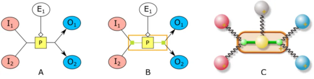
Fig. 5. How a process with two substrates, two products, and one effector node should be displayed in an SBGN-PD map (A). How our algorithm internally represents such a process using newly introduced dummy port nodes (smalled filled squares) and edges, and process container compound node (unfilled rectangle) (B). Associated physical model of our algorithm (gravitational fields not shown for brevity) (C).
Fig. 6. Illustration of how the orientation of a process might affect layout: original orientation is left-to-right by default (A), left rotation by 90 degrees (bottom-to-top) eliminates self crossings (B), and another left rotation by 90 degrees (right-to-left) further improves layout (C).
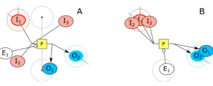
Fig. 7. Rotational force acting on process P is calculated using the angles neighboring nodes make with their connection points. A sample process with three
neighbors, where dp(dsor de) represents the desired location of an input node (output node or effector node) (A). The angles that these neighbors make with
the process node with respect to the current orientation (B). Illustration of how the signs of these angels are calculated using the left-turn rule. In this example, a left turn is assumed to signify a negative sign (C).
The idea is not to interfere with the placement of “hop” nodes that are of degree two or higher but bring any degree one nodes, which are “free” to move without affecting the overall structure of the spring system, closer to such high degree nodes. This should not only help with satisfying the SBGN-PD convention with respect to properly gathering substrates (products) together but also speed up convergence. Consequently, we periodically identify a substrate (product) node with highest degree and place any degree one substrate (product) node near it. In order to avoid any extreme amounts of repulsion forces and exploit the power of randomization, we place degree one nodes randomly within a circle centered at this highest degree node (Figure 9).
Ideally, an effector should be placed in between products and substrates. The location enhancement heuristic is similarly performed on effector nodes to avoid an effector node getting “stuck” among product (substrate) nodes. Consequently, once in a while, we pull all effector nodes near their ideal position. Notice, however, that for each orientation of a process, there will be exactly two ideal locations for effectors. For instance, for a process oriented from left-to-right, these are vertically aligned with the center of the process, one being on top of the process, and the other on the bottom, both separated from the process by ideal edge length. Again, we opt to apply a minimal amount of randomness rather than placing them on the exact ideal position for the same reasons explained earlier (Figure 9).
Fig. 8. An example, where a rotation is needed but not detected by the heuristic used for 90-degree rotations defined earlier (A). The same process, after its ports are swapped via a 180-degree rotation (B).
Modifications on CoSE
In order to properly handle process nodes and satisfy SBGN specific constraints on them, we first add a new, second phase to the CoSE algorithm, and decrease the number of iterations CoSE performs in the first phase since a “draft” layout should suffice. Starting with this draft layout, the new phase is responsible for addressing SBGN rules without ruining the resultant layout, which is assumed to satisfy generally accepted layout criteria. The difference between the SBGN phase and earlier one can be summarized as follows. Since the SBGN phase is expected to make localat Bilkent University on December 18, 2015
http://bioinformatics.oxfordjournals.org/
Fig. 9. An example, where locations of substrate, product, and effector
nodes (A) are enhanced using our heuristic (B). Higher degree nodes I1
and O2are chosen as seeds for substrate and product nodes, respectively.
The effector E1is closer to the bottom of the two ideal positions for the
left-to-right process P it is associated with.
changes in the layout, the system starts out from a lower cooling factor. Rotational forces are calculated for each process node on top of the spring, repulsion, and gravitational forces calculated by CoSE. To represent process nodes and their ports with newly introduced dummy nodes, associated CoSE method needs to be expanded as in Algorithm 1. Hence, the convergence is no longer solely dependent on node movements going below a certain threshold. We also try to ensure that all substrates and products of every process are properly oriented (Algorithm 2).
Algorithm 1 Moving nodes and applying rotation
1:function
CALCN
ODEP
OSITIONSA
NDS
IZES(C)
2:rotationList ← ∅ //candidates for rotation
3:
for all process node P ∈ V (C) with ports p
iand p
odo
4: TRANSFERF
ORCES(P )
5: RESET
F
ORCES(P , p
i, p
o)
6:
end for
7:
if (phase = SBGN )∧(totalIter%rotP eriod = 0) then
8:for all process node P ∈ V (C) do
9:
if
NEEDSR
OTATION(P ) then
10:
rotationList.add(P )
11:
end if
12:
end for
13: ROTATE
R
ANDOMO
NE(rotationList)
14:
end if
15:
C
OSE.
CALCN
ODEP
OSITIONSA
NDS
IZES(C)
16:end function
Packing disconnected nodes
Disconnected nodes come up quite frequently in SBGN-PD diagrams, especially with molecular complexes, where members of a molecular complex are all degree zero. In fact, a molecular complex might be recursively defined from another one, resulting in potentially arbitrary levels of nested disconnected nodes. Thus, any algorithm to tightly pack molecular complex members could work bottom-up, and could be easily implemented recursively. Disconnected nodes outside molecular complexes, on the other hand, are highly unlikely but not impossible to come across.
This problem is a special case of the popular rectangle packing problem discussed earlier. Various techniques such as tiling and polyomino packing have been used in the past to solve this problem in the context of graph drawing. Since polyomino packing results are superior only with larger number of nodes, as will be shown later on, we went with tiling due to its simplicity for implementation and faster running time. Notice that, most of the time, the number of rectangles to be packed is only a few and all with
Algorithm 2 New second (SBGN-PD) phase
1:function
DOP
HASE2(C)
2:
totalIterations ← 0
3:
initialCoolingF ac ← c
cool//start cooler
4:while totalIter < maxIter do
5:
totalIter ← totalIter + 1
6:
if totalIter % apprP eriod = 0 then
7: APPROXIMATEL
OCATIONS()
8:
end if
9:
if
CONVERGED() ∧
EDGESP
ROPERO
RIENTED() then
10:
break
11:
end if
12: UPDATE
B
OUNDS(C) //resize compounds
13: CALCS
PRINGF
ORCES()
14: CALC
R
EPULSIONF
ORCES()
15: CALCG
RAVITATIONALF
ORCES()
16: MOVE
N
ODES() //move nodes based on total forces
17:end while
18:
end function
similar dimensions. Hence, use of a complicated algorithm is unlikely to produce significantly more compact drawings.
Packing can be integrated into SBGN-PD layout without interference as a pre-processing step as explained in the Supplementary document. We would also like to remark that packing should only be applied to a compound node with no edges (intra-graph or inter-graph edges) in it. Any non-degree zero node contained in a compound structure should not be forced to a location determined by a packing algorithm but rather should be free to move near its neighbor(s).
Further compaction
After application of a packing algorithm, it is common to have more room for improvement, which can be achieved by calculating the visibility graph of the disconnected set of nodes to be packed. A visibility graph in a certain orientation, for example bottom-to-top, is adirected acyclic graph(dag) and represents the visibility of each node when
“looked” from that node vertically towards the up direction. We say that node v is visible by node u in bottom-to-top direction if v is above u, and u can completely “see” node v with no obstruction in between two nodes, looking from bottom to top. In other words, the nodes directly below, to the right or to the left of a node u are not visible by u. Using the directed acyclic structure of visibility graphs, a topological sort is applied to get the objects in order, and one by one in the computed topological order, each object is moved closer to its ascendant.
Even though application of this algorithm in either one of four directions might produce more compact drawings, the improvements are usually minimal if any. Also notice that a separate calculation of the visibilities is required for each direction.
Running time
CoSE algorithm runs in O(k · (|V |2+ |E|)) time, where the underlying
compound graph is represented with C = (V, E, F ), and k is the number of iterations needed to converge. This is due to the simple fact that, in each iteration, repulsion forces are calculated between each node pair and spring forces are calculated for each edge. Additional heuristics employed by our algorithm do not increase the asymptotic running time since rotational forces are calculated for each process node. Similarly, packing is linear in the number of nodes to be packed, which is at most as many as all the nodes in the compound graph. Our experiments as described in the next section confirm this theoretical running time analysis.
at Bilkent University on December 18, 2015
http://bioinformatics.oxfordjournals.org/
Fig. 10. Comparison of the success of our algorithm with CoSE (graph size vs. ratio of properly oriented substrate, product, and effector edges)
4
IMPLEMENTATION AND RESULTS
We implemented SBGN-PD layout within an open source layout library called Chisio Layout (ChiLay). The experiments outlined below were
performed on an ordinary PC (with Intel® Core™ i7-4600U 2.10GHz
processor, 8GB RAM, and 256GB SSD). For each measurement for a layout algorithm, 10 executions were performed and the average was taken since spring embedders start out from random initial positions, and this might highly affect the convergence speed.
Packing
For comparing tiling and polyomino packing methods, random compound graphs with no edges were generated. Details of these can be found in the Supplementary document. Further compaction through visibility is usually of no use with tiling. More importantly, as can be seen from the results, polyomino packing has a clear advantage over tiling with large number of nodes (> 60) but for smaller graphs, like SBGN-PD maps, tiling performs just as well.As our tests confirm, tiling is significantly faster than polyomino packing. However, since SBGN maps have relatively small number of nodes, running time spent on packing is negligible.
Parameter tuning
Our layout algorithm has a number of parameters to customize its behavior. We tested the behavior of our algorithm with respect to each such parameter and applied a comprehensive test to fine-tune it.In order to perform these experiments, we used 34 “real-life” SBGN-PD maps as taken from Pathway Commons (Cerami et al., 2011) database, using querying and conversion (to SBGN-ML) facilities of Paxtools (Demir et al., 2013). These maps were chosen to be of varying types including regulation and signaling networks, not larger than a few hundred nodes. For larger graphs, at least one complexity management technique can be used (Dogrusoz and Genc, 2006).
The main criterion used for the success of the algorithm is the ratio of “properly oriented” edges to total number of edges in the graph. To decide when an edge is properly oriented, we use a parameter named
angle tolerance(at). Other parameters of our algorithm are approximation
distance(ad), approximation period (ap), rotation period (rp), 90-degree
rotation force threshold(c90), 180-degree rotation ratio threshold (c180),
and phase 1 maximum iteration count (ip1).
Before experimenting with individual parameters, we wanted to find the most coherent set of values of these parameters given a discrete set of values for each parameter as specified earlier. The best results are obtained when ad = 50, ap = 211, rp = 2, c90 = 70, c180 = 0.5, and ip1 = 200. To confirm that changes in these parameters do not interfere with each other, we performed tests where only one parameter at a time was changed. The results can be found in the Supplementary document along with other details.
Comparison with CoSE
We have compared the success rate of our algorithm in properly orienting edges with the generic algorithm CoSE. As Figure 10 shows, there is a clear advantage of using the extra heuristics.Fig. 11. Comparison of the running time of our algorithm with CoSE (graph size vs. execution time in milliseconds)
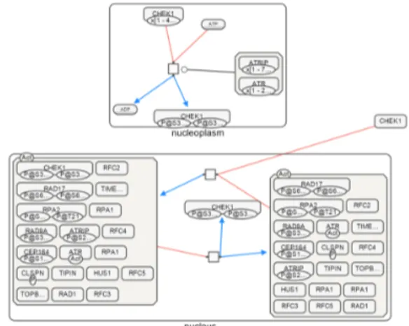
Fig. 12. Paths between ATRIP and CHEK1 as laid out by our algorithm
In terms of execution time, our algorithm performs as well as
CoSE (Figure 11). Actually, as the iteration count required to complete phase 2 increases, the number of rotation operations needed by our algorithm increases as well. However, since our algorithm applies tiling to disconnected nodes and ignores such nodes during layout, the decreased graph size seems to compensate for the extra time used by newly introduced heuristics.
We also investigated whether or not the behavior of our algorithm depends on graphs being simple or not. Our experiments show that when there are no compound structures in the graph, ratio of properly oriented edges goes up even further to around 95 percent.
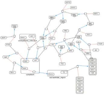
Figures 12 and 14 show sample SBGN-PD maps laid out using our algorithm using SBGNViz, which is a specialized visualization tool developed for SBGN process description maps (Sari et al., 2015). More examples are available in the Supplementary document.
The success of a spring embedder layout algorithm relies on the density of the graph more than it does on the number of nodes in the graph. For instance, even when there are a small number of nodes in a map, high connectivity in a small part of the map might make it impossible to successfully orient the edges in that part.
Figure 14 illustrates the fact that, some substrate and production nodes of a process node may be placed in another compound node (cellular location). During layout, the location of this compound node is determined with respect to the forces acting on it. Those additional forces may disrupt the proper orientation. This is a typical example, where multiple conflicting constraints are impossible to satisfy.
at Bilkent University on December 18, 2015
http://bioinformatics.oxfordjournals.org/
Fig. 13. Vitamins B6 activation to pyridoxal phosphate as laid out by our algorithm; all edges were properly oriented
Fig. 14. Aspirin blocks signalling pathway involved in platelet activation as laid out by our algorithm
5
CONCLUSION
The main motivation behind this study was to build a specialized
automated layout algorithm for process description maps that
comply with the conventions in SBGN-PD maps. Our proposed
algorithm adds the necessary heuristics to achieve this on top of a
compound spring embedder algorithm named CoSE.
The first enhancement provides proper packing of complex
members and disconnected molecules by using two different
rectangle packing algorithms: tiling and polyomino packing. The
second one supports port nodes and provides rotation ability for
process nodes by introducing a new force type. An important
point to note here is that, those enhancements are added without
disturbing the force-directed structure of the algorithm. There is
still room for improvement, however, especially in handling special
cases such as irreversible processes.
Our proposed layout algorithm has been integrated into Chisio
Layout (ChiLay) library, which is also available through Paxtools.
ACKNOWLEDGEMENT
The authors thank Dr. Debbie Bemis for critical reading of the
manuscript.
Funding: This work was supported by the Scientific and
Technological Research Council of Turkey (grant [#111E036] to U.
D. and a scholarship to B. G.), and by NIH grants [#U41HG006623]
and [#P41GM103504].
Conflict of Interest: none declared.
REFERENCES
Battista, G. D. et al. (1998). Graph Drawing: Algorithms for the Visualization of Graphs. Prentice Hall PTR, Upper Saddle River, NJ, USA, 1st edition.
Cerami, E. et al. (2011). Pathway commons, a web resource for biological pathway data. Nucleic Acids Research, 39(suppl 1), D685–D690.
de Berg, M. et al. (2008). Visibility graphs. In Computational Geometry: Algorithms and Applications. Springer-Verlag, 3rd edition.
Demir, E. et al. (2013). Paxtools: A library for accessing, analyzing and creating biological pathway data. PloS Computational Biology, 9(9), e1003194.
Dogrusoz, U. (2002). Two-dimensional packing algorithms for layout of disconnected graphs. Information Sciences, 143(1-4), 147–158.
Dogrusoz, U. et al. (2002). Graph visualization toolkits. IEEE Computer Graphics and Applications, 22(1), 30–37.
Dogrusoz, U. et al. (2009). A layout algorithm for undirected compound graphs. Information Sciences, 179, 980–994.
Dogrusoz, U. and Genc, B. (2006). A multi-graph approach to complexity management in interactive graph visualization. Computers & Graphics, 30(1), 86–97. Freivalds, K., Dogrusoz, U., and Kikusts, P. (2001). Disconnected graph layout and
the polyomino packing approach. In P. Mutzel, M. J¨unger, and S. Leipert, editors, Graph Drawing, pages 378–391. Springer.
Funahashi, A. et al. (2003). CellDesigner: a process diagram editor for gene-regulatory and biochemical networks. BIOSILICO, 1(5), 159–162.
Garey, M. R. and Johnson, D. S. (1979). Computers and Intractability: A Guide to the Theory of NP-Completeness (Series of Books in the Mathematical Sciences). W. H. Freeman, San Francisco.
Junker, B. H., Klukas, C., and Schreiber, F. (2006). VANTED: a system for advanced data analysis and visualization in the context of biological networks. BMC Bioinformatics, 7(1).
Larkin, J. and Simon, H. (1987). Why a diagram is (sometimes) worth ten thousands words. Cognitive Science, 11, 65 – 100.
Le Nov`ere, N. et al. (2009). The systems biology graphical notation. Nature Biotechnology, 27(8), 735–741.
Sari, M. et al. (2015). SBGNViz: a tool for visualization and complexity management of SBGN process description maps. PLoS ONE, 10(6), e0128985.
van Iersel, M. P. et al. (2012). Software support for SBGN maps: SBGN-ML and libsbgn. Bioinformatics, 28(15), 2016–2021.
at Bilkent University on December 18, 2015
http://bioinformatics.oxfordjournals.org/