£ к'ЧК^Ѵ;.· ■;': V Ѵ/'-'і'·» Ц У * ^ - И ··■' "■ -.ѵ/і ■·■·).■*,: ; >”Ѵ;·;· ; ' л г-■ ■¿¿/ і і ІЯІ«' w ' « !-«■‘G-Ä«”’-* 1* ѵ^· 'j'¿ aifUbi·' i ^ ’··»« ^ ψ-u >' '^í*'?:.:r\'fi-> !» íí? г- **!^·' ^••‘· ^ ·* ■■«АІИ'ІІ 4. J >t’ W î · i w A ' Ä Ä ■." ^ν ::^ ;гл . .·· ■л 4 N ëi‘^4. ^·· гл -i Λ ¿ ’ ! / ‘ '«,¿'’'- * '¿ í· ·'· 'i . « ’ и « ’ 4 « i·■«■ Д ^ r í'“4 ; ;¿j·.· .. 'Ч"; :;?x 'í:·. .; \', ^ <i ¿ ·« «.' 1»** M -;5й » 1ЛМ‘ .Ч-' İ../4 VÎ T '.Té* > ', . . . * ·. G\ 'G'/^-ÍVv G ·> : ■ -i ’.■«»··;.? > r’ . ■' ■.>·'■*' . í" « ; ¿ Ä -.- i.« * M*K'-ua.->··^ Я ·« - í«a .>.·_, ѵ;>і;;:г· ^ .'·.· v,*'-' :ji , .ул :· ■* ■■ ■ \ 'У ' >···' ’· бич íirf *»s . ,··■ а» · * -. *-. -.»♦* *»^л-T«»-.»· i»* ^ ?/frt 1^^.' .V'?<·.4'^ >’■'1*^'’ ".'■ >■'· •i'*'*t‘ ·” ■ ί»· ä: !*'■»■ Ä,· ... .„as г 8 5 Ш З л - М
INPUT SEQUENCE ESTIMATION AND BLIND
CHANNEL IDENTIFICATION IN HE
COMMUNICATION
A THESIS
SUBMITTED TO THE DEPARTMENT OF ELECTRICAL AND ELECTRONICS ENGINEERING
AND THE INSTITUTE OF ENGINEERING AND SCIENCES OF BILKENT UNIVERSITY
IN PARTIAL FULFILLMENT OF THE REQUIREMENTS FOR THE DEGREE OF
MASTER OF SCIENCE
By
lyi. Kharnes Be
J ?
7 t
б ю г . з
I certify that I have read this thesis and that in my opinion it is fully adequate, in scope and in quality, as a thesis for the degree of Master of Science.
1
Assist. Prof. Dr. Orhan Arikan(Supervisor)
I certify that I have read this thesis and that in my opinion it is fully adequate, in scope and in quality, as a thesis for the degree of Master of Science.
\ j
Prof. Dr. Enis Çetin
I certify that I have read this thesis and that in my opinion it is fully adequate, in scope and in (piality, as a thesis for the degree of Master of Science.
Assi^t^ Prof. 0 r. Murat Alanyali
Approved for the Institute of Engineering and Sciences;
Prof. *Dr. MehineyBaray
Director of Institute of En^iiieering and Sciences
ABSTRACT
INPUT SEQUENCE ESTIMATION AND BLIND
CHANNEL IDENTIFICATION IN HF
COMMUNICATION
M. Kliames Ben Hadj Miled
M.S. in Electrical and Electronics Engineering
Supervisor: Assist. Prof. Dr. Orhan Ankan
August 1999
Recent, advances in blind channel equalization approiiches and the availabil ity of fast processors have made it, possilile to communicate reliably over long distances through HF communication links. Current research efforts focus on the improvement of the performance of the communication systems which de grades significantly during the “bad tropospheric conditions” when the channel characteristics show rapid variations.
In order to improve the performance of the HF communication links during these conditions, algorithms that can identify and track the channel charac teristics are proposed in this thesis. Detailed simulation based comparisons with the existing algorithms show that the proposed approaches significantly improve the performance of the communication system and enable us to utilize HF communication in bad conditions even at 10 dB SNR.
Keywords: Blind diannel ideiitiiication, blind signal estimation, Kalman Filter,
subspace tracker, fractional sampling.
ÖZET
GİRİŞİ BİLİNMEYEN İLETİŞİM KANALLARININ HATASIZ
TANINMASI
M. Khames Ben Hadj Miled
Elektrik ve Elektronik Mühendisliği Bölümü Yüksek Lisans
Tez Yöneticisi: Yrd. Doç. Dr. Orhan Arıkan
Ağustos 1999
Gözü kapalı olarak kanal flenklc.'jtirrne konırsunda yakın zamanda geliştiriliniz olan yeni yöntemler lıızlı sayı.sal i.şlemcilcr sayesinde kullanılarak HF linkleri üzerinden güvenilir şekilde haberleşmeyi olanaklı kılınışlardır. Dvaın etmekte olan araştırmalı· iletişim ]ieribrmansmm önemli ölçüde düştüğü kanal karak teristiğinin hızlı değişim gösterdiği kötü atmosferik şartlarda artırılabilmesini arnaçlamaktadir. Bu tezde HF linkleri üzerinden yapılan iletişimin perlör- mansmı artırabilmek amacı ile HF kanalım tanıyabilecek ve zaman içerisindeki değişrnini takip edebilecek yöntemler önerilmiştir. Var olan yöntemler ile yapi- lan benzetimlere dayalı detaylı kıyaslamalarda geliştirilen yöntemlerin önemli bir performans artırımı sağlayarak kötü atmosferik şartlarda İÜ dB sinyal- gürültü oranında dahi iletişimi olanaklı kıldıkları gözlenmiştir.
Anahtar Kelimeler. Gözü kapalı kanal tanınması, gözü kapalı ters evrişim,
sistem tanınması, kesirli örnekleme
ACKNOWLEDGMENTS
I would like to use this o|)portunity to express my deep gratitude to iny supervi sor Assist. Prof. Dr. Orhaii yVnkan for his guidanee, suggestions and invaluable encouragement throughout the development of this thesis.
I would like to thank Prof. Dr. Enis Çetin and Assist. Prof. Dr. Murat Alanyali for reading and commenting on the thesis.
I express my s])ec.ia.l thanks to my family for their constant support, patience and sincere', love.
Contents
1 IN T R O D U C T IO N 1
2 A N OVERVIEW OF HE CO M M UNICATION 5
2.1 A Typical HF Communication System 5
2.2 A Model for the Communication System... 7
3 BLIN D ESTIM ATION OF IN P U T SYMBOL SEQUENCE A N D ID ENTIFICATIO N OF THE CHANNEL R E SPO N SE 10
3.1 Input Sequence E stim ation... 11
3.1.1 Estimation of Input Sequence in the Presence of a Chan nel E stim ate... 12
3.2 Blind Channel Identification... 15
3.2.1 Channel Identilication in the Presence of Input Secinence
Estimate 17
3.3 Proposed Algoril.lmis and their Simulated Performances... 24
4 SIM ULATION 32
5 CONCLUSIONS 35
A P P E N D IC E S 41
A N oise R eduction Due to Fractional Sampling 41
B Convergence of Input Sequence Estim ator 43
C P roof of Equation 3.12 45·
D R eduction in the Com putational Cost of the Kalman Filter 47
List of Figures
2.1 Surface ionospheric layers’ model... G
2.2 Diffused ionospheric hxyers’ model. 7
2.3 Model of the communication system with fractional sampling. 8
2.4 Multi-channel filter model of the baseband equivalent of the communication system... 8
3.1 Block diagram of the iterative solution... 12
3.2 Efficient implementation of the signal estimator... 14
3.3 Available samples of hM/2,71 aie shown with ‘o’. The required samples of which are shown with ‘-l·’, can be interpolated by using a low order interpolator such as linear 3-point interpolator. 20
4.1 Normalized channel estimation error in the open-eye case with
rapid time-variation and low SNR. 33
10 in the l)lind case with rapid time-variation and low SNR. .34 4.2 Bit-error and normalized channel estimation error for Algorithm
List of Tables
3.1 Average logarithmic error (in dB), Ca,,, in the case of known input seciuence for algorithms 1, 2, 3, and 4... 30
3.2 Average logarithmic error (in dB), e„„, in the case of unknown input secpience for algorithms 1 , 2, 3, and 4 30
3.3 Bit-error rate for algorithms 1, 2, 3, and 4. 30
3.4 Averagt! logarithmic error (in dB), in the case of known input sequence for algorithms 5, 6, 7, and 8. ... 30
3..5 Average logarithmic error (in clB), e„„, in the case of un known input sequence for algorithms 5, 6, 7, and 8. 30
3.6 Bit-error rate for algorithms 5, 6, 7, and 8. 31
3.7 Average logarithmic error (in dB), e„„, in the case of known input sequence for algorithms 9, 10, 11, and 12. 31
3.8 Average logarithmic error (in dB), e«,,, in the case of un known input sequence for algorithms 9, 10, 11, and 12. 31
3.9 Bit-error rate for algorithms 9, 10, 11, and 12. 31
4.1 Average logarithmic error for algorithms in [1] and [2] 33
Chapter 1
IN TR O D U C TIO N
Digital communication systems usually suffer from inter-symbol interference, ISI. This plienomenoii is known to be caused by the channel memory, which spreads the transmitted symbols in time, or due to time-varying multi-paths. To combal, the limitation in perfbrraauce due to such factor, blind channel equalizers are usually built within receiv(!rs. The blind equalization techniques proposed in the literature, either perform direct equalization, which is the case of decision feedback equalizers, DFE, [3] [4], [5], or divide the problem into blind channel identification , BCI, and blind signal estimation, BSE, [G], [7] [8] [9] [10]. The channel identification is based either on statistical jiroperties of the receivcid secpience [6], [9], or on subspace methods, mainly in the ca.se of multi-channel systems or fractionally spaced channels. In [10], a revimv, describing the main ideas behind statistical and deterministic approaches in BCI, is presented.
In this work, we address the problem of blind equalization for HF channels. These are mainly characterized by time varying paths and additive noise. The time variation in the channel response leads to a degradation in the perfor mance of the equalizer as time progresses. As a result, a periodic transmission of a training sequence is required, which means a poor management of the channel bandwidth. Moi(;over, even with the use of such periodic sequences, the ecpializer ina.y fail and result connection break-down in j)oor conditions.
Recent r(;s(;arch in the subject, tried to come up with robust equaliz ers [2], [1 1 ], a.nd (,o avoid training sequences [4]. Different apinoaches like improvements of decision feed-back equalizers and adaptive algorithms were proposed. A commonly used technique is fractional sampling [10]. The latter provides channel diversity which helps for better tracking of the variation in the channel impulse response. Moreover, with the use of an appropriate low-pass filter, the fractionally spaced channels’ output noise will have a considerably reduced va.riance.
In this thesis work, we propose distinct iterative ap])ioaches, assuming a fractionally s[)a.ce(l model of the channel, that aim a robust HF channel equal ization. Starting with a training period, a reliable estimate of the channel can be obtained. Then at each iteration, we make use of the previous channel es timate to predict the input symbols and then use them to update the channel transfer function estimate. To ensure the convergence of the equalizer over a long period, we develoijed a K-dela.yed input sequence estimator that mini mizes the cumulative mean square error over the last K output measurements. We also suggest different algorithms for the channel identification purpose.
The chaiiucl identifier eonsists of a cascade of two different blocks. The first is a Kalman filter that makes use of the estimated input vector to provide an estimate for the channel impulse response. The latter will be fed to a subspace tracker to update an estimate for a basis of the channel subspace. Once a reliable estimate is ol)ta.iiK!d, significant part of the noise can be eliminated through a projection. The described approach is based on the assumption tha.t the slowly tiuKi va.rying channel belongs to a low-rank subspace. Based on different descriptions of the problem, distinct channel identification methods are develo|)(xl.
Anotlnu· relevant issue in HF communication is the modeling of the HF system. Any i>roposed model should reflect the physical characteristics of tlie transmission medium. A simple and commonly used model, proposed in [12], reflects the multi-])ath nature of the HF channel and the randomness in path delays and amplitude distortion. As a part of our contribution, we extend the described model a more realistic one that takes into account the limited bandwidth of the channel and the physical characteristics of the reflective iono spheric layers.
The j)roposed approaches are simulated for different noise realizations and time-variation conditions. The performance of the channel identification algo rithms is toîsted in both, blind and open-eye, cases. In the case of known input sequence, all the proposed algorithms show rapid convergence and relatively small estimation error.
The organization of the thesis is as follows: First an overview of the HF communication is given and the new HF system model is described. In Chapter 3, the problem formulation is presented. Then, a description of the input
sequence esl,iinat,or is provided. The different channel identification methods are explained a,nd tlie algorithms are explicitly stated and compared in terms of performance and computational cost. In Chapter 4, simulation results of the best performing algorithms are shown and compared to the ones corresponding to already existing approaches. Finally, the thesis is concluded.
Chapter 2
A N OVERVIEW OF HE
COM M UNICATION
2.1
A Typical HF Com m unication System
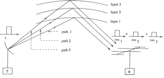
In HF communication, tlie transmission medium in between the transmitter and the receiver s,ystems is the atmosphere. Transmitted signals may follow multiple paths as they are reflected by distinct ionospheric layers. A siinide model for such channels was proposed in 1969 by Watterson [12], and exper imentally verified in 1970, [13]. The model represents each signal i)ath by a delayed impulse, the magnitude of which changes in time to reflect the random nature of the rcdlections in the ionosphere. In the Watterson model, surface ionospheric la.yers are assumed to be as shown in Figure 2.1, and each transmis sion path is represented by a single delayed impulse. As a result, the individual reflections in each multi-path ma.y cause amplitude distortion and dehiy but
do not diange tho?, shape of a the transmitted signals. Therefore, the baseband
Figure 2.1: Surface ionospheric la3^ers’ model.
channel I/O equation for the Watterson model can be written as;
y{t) = (2.1)
i
where G,;(/;) models the time vaiying reflection and it is obtained by filtering white noise with a Gaussian function.
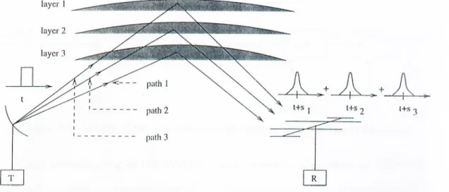
An imi)rovement of the Watterson model can be obtained by incorporating diffuse reflective layers to the model (see Figure 2.2). This can be achieved approximately by modeling the channel transfer function as a sum of shifted Gaussian functions, each of which corresponding to a distinct transmission I)ath. The intuition behind such a choice is the assumption that the reflection points are independent and identically distributed in the space occupied by the ionospheric la.yer. The improved baseband channel model becomes:
vC) = T,Gi{t)\x(t) * h(t - s,)\ (2.2)
i
where /¿(i) = and (*) denoting the convolution operation. By choosing the shape: G,//;) and 7i, and location: Sj, parameters of each channel
l+S '
Figure 2.2: Diffused ionospheric layers’ model.
transfer function as time-varying, various important physical characteristics of the HF channels such as the altitude and the thickness variations in the reflective layers can be modeled.
2.2
A M odel for the Com m unication System .
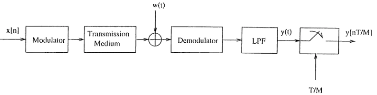
A typical HF communication vsystem with serial data-transmission can be mod eled as shown in Figme 2.3. The input data symbols x[n] are chosen from a finite alphaljet. The transmission medium is the atmosphere, as previously described, and y{t) and w{t) are, respectively, the received and additive noise signals. Following the demodulator, the signal is low-pass filtered with a pass- band equal to that of the input signal bandwidth. Then the output of the low- pass filter is sampled with an over-sampling factor of M where T corresponds to the ini)ut symbol duration. The channel transfer function is assumed to be the cascade of the transmitter filter, the transmission medium, and the receiver filter.
w(l)
^I7M Figure 2.3: Model of the communication sy.stern with fractional sampling.
The ()versa.ni|)ling of the receiv(',d signal, which is also called as fractional sampiling, resvdts in channel diversity. In [14], it is shown that using iractional sampling, the commnnication system model becomes equivalent to a single input multiple-output, SIMO, system as shown in Figure 2.4. This technique was extensively exploited in the literature, and the identifiability conditions for fractionally sj^aced channel are considered in [15] and [16].
xl'vl
y. In]
y2 l‘'l
t"'
M
Figure 2.4: Midti-channel filter model of the baseband equivalent of the com munication system.
In Figure; 2.3, the noise signal w(i) is low-pass filtered and then fractionally sampled to get the noise sequences u,;[n], i = 1, . . . , M, shown in Figure 2.4. In Appendix A, we sliow that the low-pass filter,LPF, together with the fractional sampling t.cclmifiue reduce the noise variance by a factor of 1/M. Moreover the noise sanqilcs become correlated and the noise covariance matrix acciuires a special form that deiiends on the LPF impulse response. Assuming a known noise variance, the noise covariance matrix can be precomputed. The required noise statistics can be estimated during silent intervals, or even during data transmission by computing spectral energy of the demodulator out[)ut out of the spectral siqiport of the signal.
In this thesis we will address the following problem: given the output mea surements ;i/t[n], i = 1, 2, . . . , M, and the second order statistics of the additive noise proce.sses u,:[n], obtain reliable estimates to the input sequence
and the channel transfer functions (see Figure 2.4) .
In the following cha])ter, this problem will be treated in detail and the proposed algorithms will be presented.
Chapter 3
BLIND ESTIMATION OF
IN P U T SYMBOL SEQUENCE
A N D IDENTIFICATION OF
THE CHANNEL RESPO NSE
In HF coiuimuiicalion, as in rnosl, of the communication systems, the ultinnite purpose is to l)(i alrle, to estimate the transmitted symbol sequence as relialde as possible at the receiver. However, since the medium of transmission is the HF tropospheric channel, the receiver has to provide estimates to the input sym bols in the absence of a jnecise channel transfer function. This problem is faced also in the. mobile communication systems and has been commonly reterred to as the problem of “ blind estimation of the input symbol sequence”. Another important problem in the HF communication is the identification and tracking of the time-varying HF channel response when the channel input sequence is
unknown. This laUer problem is commonly referred to as “blind channel iden tification” and has found application in many other communication systems. As it can be expected the blind channel identification and input sec]uence esti mation problems are very much related to each other, and in most apiilications a solution to one of them requires a solution to the other one. Therefore in the approaches proposed in this thesis, the problems of blind channel identifi cation a.nd input symbol (istinmtion are iteratively solved by making use of tin; solution to oiui 1,0 get a solution to the other.
3.1
Input Sequence E stim ation
In this section, wc. describe a method to estimate the input symbols when they are chosen from a binary alphabet. Assuming that the individual channel responses are of finite duration: hi,„ = [hi,u[0],/b,n[l],... , /b,n[A — 1]]'^ ,where L is the channel order, the individual channel outputs can be written as:
ViM = h^’,x„ -b w,:[n] (3.1) where x„, = [ ; i ; [ n ] , - 1],... ,.x[n - L -|- 1]]'^’ is the channel input vector. Now, a precise statement of the problem can be given as:
estimate .'¿[n] G {T^}) for n > 0
by usiruj ;(/i[n] = + for I < i < M.
As seen in the alrove formulation, the available measurements yi[n\ depend on on the unknowns of the problem: Xn and in the multiplicative form. Hence, the input sequence cannot be reliably estimated by using efficient estimators such as the Kalman filter.
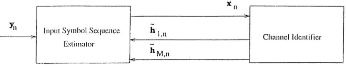
In (,lu; following, we will i)iovide alternative solution approaches where, after obtaining an initial estimate to the channel by using a short training- period in which a known sequence is transmitted, the input sequence will be estimated by using the estimated channel and then the channel estimate will be updated by using the estimated input seciuence. A block diagram for this iterative solution tcchniciue is shown in Figure 3.1.
Figure 3.1: Block diagram of the iterative solution.
3.1.1
E stim ation of Input Sequence in the P resence of
a Channel E stim ate
In this section, we will consider the estimation of the input sequence by as suming the availability of a reliable channel estimate h„. The statement of the input sequence estimation problem becomes:
Giv(',n h,;„, and the covariance of the zero-mean noise n,:[ri];
caiiniate a\v\ G {d-A}, for n > 0
by using yi[n] = hg„,Xu + 'Wt['»'], for 1 < i < M.
Many alternativi! estima.tion techniques arc available for the ab(we problem. Alternatives include Kalman filter and Viterbi algorithm [17]. In tlu', following, we will propose an efficient but sub-optimal estimator for the input sequence estimation.
Given the i)a.st input symbols x[n - 1 ] , , x[n - L + 1], let x,\ = [/1 :f\n - 1]... x[n - L -1- 1]] '’ and xj*, = [-di x[n - 1]... x[n - L + 1]]^ be the two possible vector values of x„, whe,n :i;[n] is not known. Let , . . . , !>('· the last estimates of the sub-channels given by the channel identifier. The lattcrs can be taken as reliable estimates of hi,7,,’s as far as the channel slow-variation assumption holds. We deline the estimate of X7,, as:
M
Sin = a r y i n m ^ Uiln] - li-',._,x;^,)
7;= I
,ry = 1,2. (3.2)
Note that the (istimate of x[n] can be extracted from x„,.
In tlui case where the sub-channels are not sensitive to the present input symbol .'r[nj, i.e, /i.7;,7,[0] ~ 0, the output noise and the channels’ identifica tion error may drastically degrade the performance of the described estimator. Hence, a more rea.listic goal woidd be to estimate ;c[n — /C], < L, instead of
x[n], that is a /Gdelayed input decision.
Let x5(, q = 1 , . . . , 2^'"·'·', be the po.ssible vector values of x„. when only the input .symbols i)rior to x[n — K\ are known, i.e, x,*, = [/1... /1 :i;[n — K — 1 ]. . . x[n - L + 1]] ' ’. The estimate x„, is defined as:
M . K x„, = avfj mm Xn 1 M Jyl iv \ E iT T i E (s'·!” - *^1 - . ,f7 = l,2 ,....,2 ''-'-'. (3.3)
In the last cost function, h,:,7,,-i, i = 1 , . . . , M , are used as estimates of Such an approximation is justified by the channel slow varia tion assumption and the reliable performance of the channel identifier.
By looking at the cost function, the algorithm seems to be computation ally exhaustive. However, under the condition that x[n] G {±H}, the terms
involvo; most of the inviltiplications in the cost function, c,; a , n
be seen as a summation of the terms . . . , - 1]. If we let,
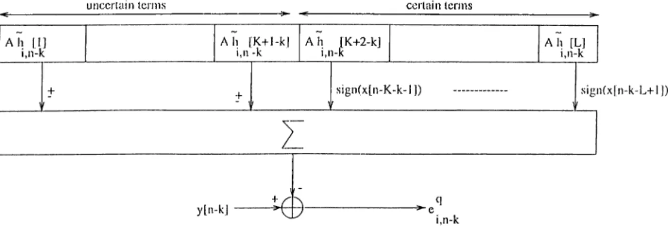
= yi['T>' - k ] - (3.4) then a simph', implementation of the hardware responsible for calculating
would be as shown in the figure below. Note that, the input .sym bols transmittc'.d prior to x[u-k] are assumed to be known because (,hc estima tor shoidd ha.ve decided on their values at previous iterations. With the de scribed imphunentation, the computational cost of the input symbol seciuence estimator can be reduced to M L + {K 4- l ) M instead of -f {K 4- 1)M multiplications.
certain terms uncertain terms
Figure 3.2: Efficient implementation of the signal estimator.
In Appendix B, the input sequence estimator is shown to converge to the correct solution. However, the output noise and channel estimation error may result in wrong decisions. In order to avoid such events, K should be chosen such tliat hi^,\K] is as large as possible for i = I , . . . , M. A safe choice would be K > arguMiXj /g:,„.[j] or even a close value would be fine.
3.2
Blind Channel Identification
The prol)lcm of l)liiid chaiiuel ideiifificatioii has a variety of applicafioiLS such as blind eciuaJizafioii of eommunicafion systems, seismic data processing, speech processing, and image roistoration. In all these applications, the channel iden tification hel])S overcoming a distortion phenomenon and estimating an origi nal signal. FurtlKuinore, blind identification of tropospheric channels helps to probe into tlu'. physical characteristics of the troposphere [18], [19].
In this sec’.tion, we focus on the case of noisy and slowly time-varying chan nels.Such chann(;ls are relevant, especially, in HF communications. The slow time-variation is assumed within one iteration. However, rapid variation is allowed in the long term sens.First attempts in blind equalization proposed periodic transmission of training seciuences to update the channel estimates in equal time intervals [2]. Such approaches suffer an important loss in through put and the effective channel rate may reduce to 50 % [10]. Current research on this issue a.ims at less or no use of training periods with negligible loss in the performance of the estimator. [4]. A commonly used method is the creation of redundancy and channel diversity through the fractionally spaced channel implementation described in Figure 2.4 [10]. However, even with fractional sampling, the. problem still rcciuires robust algorithms with fast converging rates in order to track the channel variation. As stated in [20], in the case of a ten-tap-weight FIR channel, to achieve convergence some of the previously proposed approaches ma.y require more than 1000 training symbols.
Given (,lu! output mca„surernents j/if/i], z = 1, . . . , M, and the covariances of the noise se(}uences ?;,;[n];
eHfirnate h,;_„ for n > 0 and 1 < z < M
by UHiruj y,[ii] - + z;,:[7z], for 1 < z < M.
Since both x„, a.nd ar<! unknown, the channels’ identification problem l)e- comcs a diflicuit task. Most of the already proposed ai>proaches assume some prior knowledge! of the input sequence.
Diflhrent methods and technieiues were exploited in the BCI problem. They differ, mainly, according to the assumed prior knowledge about the input se quence and the considered channel model. An important and commonly used class of BCI approaches is known as the subspace methods. The idea consists of minimization of the following quadratic cost function [10],
h = ar (7 min h^^Qli,
hG.S (3.5)
where li is the channel inqoulse rorsponse, which is in subspace S. Iji one
avenue of ap|)roa.cIies known as the cross relation [9], [10], the strong correla tion between channel output i)airs is exploited. Alternatively in the subspace approaches, the orthogonality property between the noise and the fraction ally spaced channel subspaces is exploited in the estimation of h [20]. These methods, together with the least squares smoothing technique, assume no prior knowledge about the input signal. In the case where the second order statistics of the input secpience are known, the cyclostationarity property of the output signal is exploited, either in the time domain [6], [21], or in the frequency domain [8], to get an estimate of the channel transfer function. In all these approach(!s, the subspace algorithms arc applied on the output sequence y[n].
Apart from the subspace methods, the maximum likelihood estimator and the moment matching techniques were also proposed as competing alternatives in J3CI problem.
In thci presence of reliable estimates to the input, adaptive filters have been used with considerable success as well [1], [2] [22], [23] . In [1], a modified fast transversal lilter is ¡noposed and shown to achieve nice performance un der the assumi^tion of correct input decision. In [2], a set of efficient channel estimators werci developed based on a state space representation that describías the chami(d as a. linear combination of the basis vectors spanning a subspa.ee. Although these algorithms do not assume the multi-channel model, their ex tension to the fractionally spaced channel is straight forward. However, they assume the periodic transmission of a training sequence. In the sinndation part, we’ll use these last two approaches as reference methods bcicause they are known to ])erform well in the case of noisy time-varying channels.
In the next section we’ll propose a set of new approaches to the channel identification problem in the presence of an estimate of the input sequence.
3.2.1
Channel Identification in th e Presence of Input
Sequence E stim ate
In this section, we address the channel identification problem in the case of available rdialrh; input sequence estimate. In other words, given x„, and the received signals //¿[n]:
(istirnate for n > 0 and 1 < ¿ < M 17
b y u s i n g 7y,:[n] = x„h,;,„ + '«¿['nj, for 1 < ?; < M.
We will propose a spectnirn of algorithms within this section. We present the proposed fi.i)])roa.ch(',s a.nd pnt them in perspective witli some of the a.lrcady existing approaches to clarify the intuition behind our contribution.
In the pro[)os(K.l a.pproaches, the time va.riation in the channel response will be tra.cked by slowly rotating the basis v(!ctors of the subspace S. Henccg we are a.ft(!r the tracking of the subspa.ce basis which will help for a Iretter tra.cking of tlui dia.nnel variation. First, by using the available ('.stimates to the input secjuence x[n], an adaptive filter is used to get an estimate h„, of the oversampled channel response vector h„. Second, a subspace tracker makes use of this estimate to update the subspace basis. Finally a more refined estimate h„, is obtained based on the updated subspace.
A formal d(;sc;rii)tion of the jjroblem is a statc-s])ace representation with the state equation,
= h„_i + b„, (3.G)
where b„, is a noise vector r(;ferring to the innovation in h„. The corresponding measurement I/O equation becomes
y„, = C„h„ + v„, (3.7) where and . . r nfi r 7 1, 1. c C' ^n,{) .t[77,] 0·^' x[n — 1] x[n — L -\-1] 0T (3.8) (3.9) 18
The zero vector separating each two consecutive input symbols in c„,o has length M - 1. The vectors are obtained by shifting the vector c„,j) i times to the right in a circular manner. In this way, the input symbols in the raw are multiplied by the tapweights corresponding to only. The output vector y„, is defined as, y„ = [y\[n] 7/2 · · · UmVAY'·
A roi)iist ('stinurtor for h„, is the Ka.lman filter which is the optimal least mean ,s(]ua.re estiiimtor [24]. However, tlu; Kalman filter requires O (p’) numl)er of operation for each new h„ estimate where p — M L. Therefore, for large p, direct use of Kalman filter ma,y be j)rohibitive.
To reduce, tlie number of operations needed in the Kalman filter, we propose a simpler statospace re])resentation. The idea consists of tracking h;^„, where
I = [ y ] , a,nd approximating the other channel realizations with three-i)oint
linear interpolations of This idea leads to the following representation of the all other sub-cliannel responses as a function of
hi,)!. - i = 1 ,2 ,..., M. (3.10)
where A,;’s are the appropriate linear interpolation operators. Thus, we only need to ob(.ain estimates for h/,,,. which can be achieved by using Kalman filter in the following reduced state-space representation:
h/,;i, — 4 ci„. (3.11)
y?i — -h V„ + rjn· (•^■1-2)
The vector d„ is a noise vector similar to b„, with dimension M x 1 instead of ML X 1, and 'ijn is a white noise vector that is incorporated to the measurement
equation to partially compensate the approximation introduced by the inter polation relation in (3.10). The measurement errors, v„, and the interpolation errors, T}n are assumed to be independent. The modified measurement matrix C„ has the ibllovving form:
(3.1.3)
In Appendix C, a derivation of equation (3.13) is given, and a simpler wa.y of computing C„, that avoids the vector multiplications, is presented.
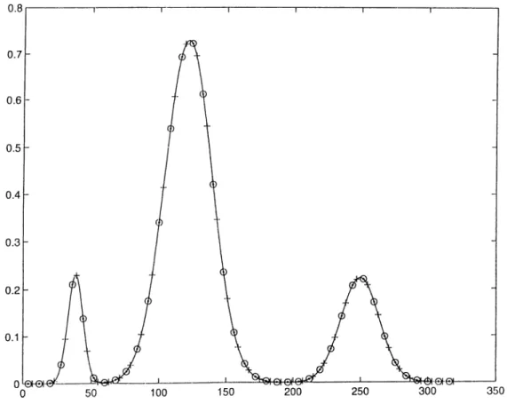
Figure 3.3: Available samples of liM/'i.n ai« shown with ‘o’. The required samples of h,:,„, which are shown with ‘-h’, can be interpolated by using a low order interpolator such as linear 3-point interpolator.
A furl,her simplification can be obtained by assuming all Aj in (3.10) as identity oi)erators. In this case, the model will have equation (3.11) as its state equation, whereas the output equation will be
.Yn ~ Cnlh,7i "h Vy, r/yj. (3.H)
where
C„,
/r
(3.15)
As shown in Appendix D, in this case the computational complexity of the Kalman filter is 0{L'^) vdiich is.significantly less than 0 {{L M Y ) of the first state space representation. Further improvements in the processing speed can be achiev(id through the systolic array imj)lcmentation of the Kalman filter as described in [251 a.nd [2
In all the previously described models, the innovation in the state vectors is modeled as an additive; white noise. This implies that its covaria.nce matrix
Qd — (.3.16)
where is the noise variance. In [27], a better formulation of Qd is pro posed. The la.tter assumes a strong correlation between the innovation and the estimated state vector. That is,
Qd — a
Ilk,.-,
II-ki 0 0 0 k,2 0 0 0 kL [.?]P + I V - -d.i (3.17)mulation, where the state vector represents the oversampled channel impulse
response, j = 1 ,2 ,..., M L, the terms - 1] and [j + 1] should be replaced by - M] and hi.,n-i[j + M], respectively. As it will be shown through the simulations, this method helps to reduce the high ireqnency noise in the estimates of the channel response.
The Kalman filter, although optimal in the MMSE sense, provides noisy estimates of the channel transfer function. To remove such a noise, we make; use of subs])a.ce tiiiddug me.thods. In other words, under the slow time-variation assumption, the matrix H = fh„,_yv · · · bn.] is of low rank. Its column space is the same; as tlu; one of which is the channel covariance matrix over a time interval of length N + 1. Hence by tracking the eigenspace of the channel covariance maluix, l)ased on the estimates given by the Kalman filter, we can remove most of the noise components. In the literature, various algorithms that can a,c.complish such a, task were proposed. Some of these are described in [28], [29], [30], a.nd [31]. The main issues about such algorithms are numerical stability; thal, is robustness to numerical error buildup, and computational complexity. In our apinoach, we chose the algorithm LORAF 1 presented in [31], which is a la.w rank adaptive filter. For our purpose, we are interested in the Suhspacc Tracking Section only. This algorithm tracks the r dominant eigenvalues of the covariance matrix = E[hn h]?,'}, and their corresponding eigenvectors. With an a])i)ropriate choice of r, the effective dimension of the subspace, most of the noise comi)onents can be eliminated from the signal. That is, if
<F = UDU'^' (3.18)
where U = [ui ... u,,] is the matrix of eigenvectors and D = diag{X\,... A,,) is the diagonal matrix of the eigenvalues. Assuming that A better approxirnant
to the covariance matrix of the signal of interest only would be;
<i>, = u ,D ,u ;
T(3.19)
where U,· = [ui ... u, ] and = diag{\\ ... A,.) assuming that Aj are indexed in decreasing order. Since the channel is time-varying, its covariance mai.rix should be tiimi-deiHmdent. For each newly available /t„ estimate, LORAF 1, performs tlm following ra,nk-one update of
d>,, = a<I>,i_i -I- (1 - o:)h„h'/(. (3.20)
To perform a slowly time-varying update of the exponential forgetting factor (X should bci chosen close to but less than 1.
Once the eigenvalues and eigenvectors are obtained, the channel impulse response can Ire re-updated in two alternative wa.ys. The first consists in ])ro- jecting h„ on to the subspace of eigenvectors.
h„ = u„u'/;h„.
In the second method we estimate h„,hj( as follows;
1
r„, (<I>„ - $„_i) (3.21)
then extract h„, from the matrix r „ as stated in the respective tabidar form of the algorithms.
3.3
P roposed A lgorithm s and their Sim ulated
Perform ances
As previously described, (;he channel identiiicaljon problem can be ibrmula(,cd in three diiieixmt state-space representations. Moreover, two diflerent forms of the innova.tion covariance matrix (3.1G) and two distinct ways of re-upda,ting the chaniuil (istimate based on the ui)da.ted subspa,ce are proposed (.3.17). The combinations of all these a.l(,(U'natives result in twelve different algorithms.
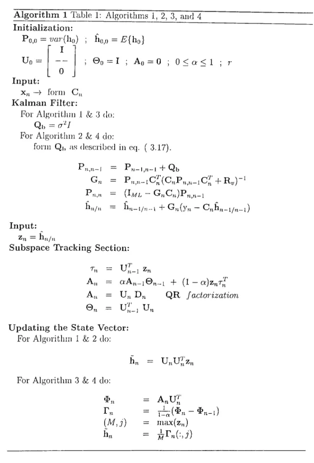
The algorithms 1, 2, 3, and 4, shown in Table 1, assume the state-space representation described by the state equation (3.6) and the output equation (3.7). In algorithms 1 and 2, the Kalman filter estimate of the channel is projected on tlui updatcal subspace, whereas in algorithms 3 and 4, the fijial estimate is obtained from F,,. as described in last section of the Table 1. The difference between algorithms 1 and 2, and similarly 3 and 4, is the form of the innovation covariance matrix Qi,.
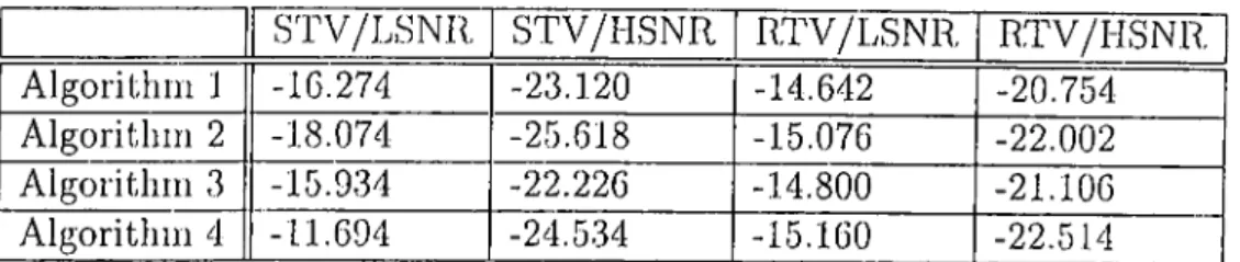
These four algorithms are compared through simulations over a one K-bit binary sequence. The fractional sampling factor is chosen as M = 8. We consider slow and rapid, in the long term sens, time-variations: STV and RTV respectively. yUso, the signal to noise ratio is chosen as 23 dB and 10 dB and represented as HSNR and LSNR respectively. Furthermore, to investigate the effect of blind seciuencc estimation on the performance of the blind channel identification we perform the simulations with both estimated and exact input sequences. In each of these cases, the results are obtained over 10 independent realizations. The error measure is defined as e[n] = 20 log and e„,„ is the mean of el?/.] in the stea.dy state.
According 1,0 the simulation results shown in Table 3.1, all of the first four algorithms show good performance in the case of known input secjuence. As expected, the increase in time-variation or the decrease in the SNR result in a larger channel estimation (uror. Based on the obtained results, the algorithms 2 and 4 outirerform algorithms 1 and 3 respectively. This fact implies that defining tlui innovation covariance matrix as described in equation ( 3.17) im proves tlie [xni'oi inance in the channel identification. Similarly, algorithms 2 and 4 outperform a.lgorithms 1 and 3 respectively in the rapid time variation case and the oi)posite becomes true when tlie channel (exhibits slow variation. This result can be explaimxJ l)y the fact that the projection onto the subspace acciuires the algorithm a large memory of the past values and a reluctancy to perform rapid updates. When the input sequence is unknown we notic:e an increase in the estimation error. The latter is due to some bit uncertainties, in the input vector, l.hat effect the i)erformanc(! of the channel identifier. How ever, even with less reliable channel estimates, the input se(iuence estimator is still capable of making the correct decision about the input symbols. Note that, as Tables 3.2 and 3.3 show, only few decision errors occured in the case where the channel is ra])idly varying and having a low SNR.
The algorithms 5, 6, 7, and 8, shown in Table 2, assume the state space representation that described l)y the equations ( 3.11) and ( 3.12). The differ ences between these algorithms are emphasized in Table 2. By examining the Tables 3.4, 3.5 and 3.6, we can notice that algorithms 5 and 6 perform better than algorithms 7 and 8 in the blind case and also when the time variation is slow, whereas the last two algorithms exhibit better performance when the input sequence is known and the channel is rapidly varying.
Algorithms 9, 10, 11, and 12 are stated in Table 3. As previously mentioned, they approximate the sub-channels with a unique one. This assumption leads to a considerable reduction in the number of computations without degrading the performance of the algorithms. In fact, from the Tables 3.7, 3.8, and 3.9 we can see that algorithms 10 and 12 can be considered as the best, in terms of elliciency and computational cost, when the input sequence is known and the chaniu',1 is rapidly varying, whereas algorithms 9 and 10 outperform all the others in the blind case or under the slow variation condition.
A lgorithm 1 Table 1: Algorithms 1, 2, 3, a,rid 4 Initialization:
Po,o =_?;ar(ho) ; ho,» = £^{ho} I i 0 0 = 1 Uo = Input: A() = 0 ; 0 < a < 1 ; 0 forai C, Kalm an Filter:
For Algoritlmi 1 & 3 do;
Qb =
F'or Algoritiiiu 2 & 4 do;
form Qi, as described in eq. ( 3.17).
Pii.,71—1 Fj/.—I,n—1 "b Qb
Pr;,,7?, = (J-ML ~ G„,C;i)P;j^yj_][
Input:
2)1 — h„y,i
Subspace Tracking Section:
Tn
Aji, · o :A „._ i© ^ ._ 1 + (1 - a ) z „ r j A „, = U „ D „ Q R fo ,c to r iza tio n
© n = u ;^ :, u „
U pdating the State Vector: For Algorithm 1 & 2 do:
u„,u;i,'2 For Algorithm 3 & 4 do:
r„, (M ,S lin = A „u ;; = rb ;(* « - * » -i) = max(z„,) 27
A lgorithm 2 Table 2: y\]gori(,hms 5, 6, 7, and 8 Initialization:
Po,o == wa7-(h(,o) i ho,() =
I Uo = — ; ©0 = I ; Ao = 0 ; 0 < a < 1 ; r 0 L -Input: x„ — > Ibrni C„, Kalm an Filter:
Fbr Algoritlun 5 & 7 do:
Qci
-For Algoridim (5 & 8 do:
forni Qc] as described in eq. ( 3.17).
—J ~ Pn—l,n—1 "b Qcl
G„, = + +
Pn,n = (1/. - GnC„)P,i^„_i
h;i,/n h,i_j^,,_i + G„,(y„.
Input: hj,y7j.
Subspace Tracking Section:
Tn =
= G: A,(_ j 0 „ _■ 1 + ( - a ) z „ r j
■^n = U7,, Dn QR f actorization
0R = u „
U pdating the State Vector: For Algorithm 5 & 6 do:
H,n
u„u;[z„,
For Algorithm 7 & 8 do:
= A„U’·
Tn =
(M ,j) = max(z,i)
h/,„
A lgorithm 3 Table 3:Algorit]ims 9, 10, 11, and 12 Initialization:
Po,o = war(h/,o) ; h(),o = A’{h/,o} Uo = Input: I 0 ibnji C,, ; © „ = I ; A o = 0 ; 0 < o; < 1 ; Kalman Filter:
For Algoriduii 9 & 11 do:
Qd = o'^l
For Algoritlun 10 & 12 do:
form Qd as d(;scril)od in (3(]. ( 3.17).
1 ri,,n—l P)i.—l,n—1 f Qcl
U f U (1/. ~ Gn.Cn)Pn,n-l
h,i/7i, h,i_ |/„_] + G„,(y„ C„,li„,_i/„_i)
Input:
' h„y„
Subspace Tracking Section:
T n = U ' - l
A n = o ; A , ^ _ i © „ _ • J. + 1; i - a ) z „ r , y A n = U „ D „ Q R f a c t o r i z a t i o n
U pdating the State Vector: For Algorithm 9 & 10 do:
h,n
For Algorithm 11 & 12 do:
= A,.u;','
r,:(M ,i) = max(z„)
= ¿ r n (:,i)
STV/LSNR STV/HSNR RTV/LSNR RTV/HSNR
Algorithm 1 -1G.274 -23.120 -14.G42 -20.754
Algorithm 2 -18.074 -25.G18 -15.07G -22.002
Algorithm 3 -15.934 -22.22G -14.800 -21.10G
Algorithm 4 -11.G94 -24.534 -15.1G0 -22.514
Table 3.1: Average logariUiinie error (in clB), in the case of known input seciucnce for algoritluns 1, 2, 3, and 4.
STV/LSNR STV/I-ISNR RTV/LSNR RTV/HSNR
Algorithm 1 -14.238 -18.132 -G.030 -14.258
Algorithm 2 -14.720 -18.543 -G.490 -18.58G
Algorithm 3 -12.431 -1G.521 -5.000 -14.1G0
Algorithm 4 -12.GG2 -1G.012 -G.304 -12.5GG
Table 3.2: Average logarithmic error (in dB), e„„, in the case of unknown input sequence for algorithms 1, 2, 3, and 4
STV/LSNR STV/HSNR RTV/LSNR RTV/HSNR,
Algorithm 1 0 0 0.034 0
Algorithm 2 0 0 0.04G 0
Algorithm 3 0 0 0.057 0
Algorithm 4 0 0 0.014 0
Table 3.3: Bit-error rate for algorithms 1, 2, 3, and 4.
STV/LSNR STV/HSNR RTV/LSNR RTV/HSNR
Algorithm 5 -18.458 -24.29G -1G.928 -20.920 '
Algorithm G -20.132 -13.184 -17.39G -21.80G
Algorithm 7 -17.774 -22.214 -17.728 -20.050
Algorithm 8 -21.154 -25.15G -17.788 -23.276
Table 3.4: Average logarithmic error (in dB), Cav, in the case of known ini)ut sequence for algorithms 5, 6, 7, and 8.
S'LV/LSNR STV/HSNR RTV/LSNR RTV/HSNR
Algorithm 5 -15.357 -18.327 -11.166 -16.000
Algorithm G -15.447 -18.701 -12.574 -14.552
Algorithm 7 -12.725 -17.328 -12.024 -16.24G
Algorithm 8 -13.013 -17.107 -10.742 -17.798
Table 3.5; Average logarithmic error (in dB), in the case of un known input sequence for algorithms 5, G, 7, and 8.
STV/LSNR STV/HSNR RTV/LSNR RTV/HSNR
Algorithm 5 0 0 0.0087 0
Algorithm 6 0 0 0.0011 0
Algorithm 7 0 0 0.0306 0
Algorithm 8 0 0 0.0077 0
Table 3.G; Bit,-error rate for algorithms 5, 6, 7, and 8.
STV/LSNR STV/HSNR RTV/LSNR RTV/HSNR
Algorithm 9 -18.256 -23.756 -17.134 -21.054
Algorithm 10 -20.280 -24.498 -17.252 -21.594 Algorithm 11 -18.880 -23.390 -17.440 -22.294 Algorithm 12 -19.266 -24.318 -18.668 -22.930
Table 3.7: Average logaritlimic error (in dB), ea„, in the case of known input sequence for algorithms 9, 10, 11, and 12.
STV/LSNR STV/HSNR RTV/LSNR RTV/HSNR
Algorithm 9 -14.980 -18.737 -10.830 -17.902
Algorithm 10 -15.872 -18952 -11.334 -19.162
Algorithm 11 -11.378 -17.262 -9.117 -18.332
Algorithm 12 -10.128 -17.023 -9.282 -18.944
Table 3.8: Average logarithmic error (in dB), e„,„, in the case of un known input sequence for algorithms 9, 10, 11, and 12.
STV/LSNR STV/HSNR R.TV/LSNR RTV/HSNR
Algorithm 9 0 0 0 0
Algorithm 10 0 0 0.0022 0
Algorithm 11 0 0 0.061 0
Algorithm 12 0 0 0.56 0
Table 3.9: Bit-error rate for algorithms 9, 10, 11, and 12.
Chapter 4
SIM ULATION
In this diaplxn, we simulate two already existing approaches and compare them with the results found in the previous chapter. The reference algorithms were proposed in [1] and [2]. The former describes the channel as a linear combination of a subspace basis. At each iteration, an iterative updating of the channel and the subspace is made. The second algorithm is a fast transversal filter.
In the simulations, the channel transfer function is a summation of three shifted Quassia,n functions, each of which represents a distinct path. The chan nel order is 40 tapweights and the oversampling factor is 8. As in the previous chapter, the algorithms are simulated over ten different realizations.
When the iniiut sequence is known, the algorithm described in [1] fails whenever the channel is rapidly varying or when the SNR is high. As shown in Table 4.1, the average error is high indicating convergence difficulties. The fast transversal filter described in [2], shows a smaller error. But when compared
STV/HSNR STV/LSNR RTV/HSNR RTV/LSNR Algorithm in [1] -17.4116 -4.841 -4.956 -4.841 Algorithm in [2] -20.826 -7.610 -7.962 -7.352 Table 4.1: Average logaii(;hmic error for algorithms in [1] and [2]
to our proposed approaches, it has a relatively inferior performance, figure 4.1 illustrates this fact.
In the blind casii, both reference algorithms diverge and do not resist injiut decision errors, wheras our proposed approches are robust to such errors, (see Figure 4.2. These results clearly indicate the superior performance of our algorithms in blind and open-eye conditions.
Figure 4.1: Normalized channel estimation error in the open-eye case with rapid tirrui-variation and low SNR.
0.5 7 0 m -0.5 -1 500 1000 1500 2000 n 2500 3000 3500 4000 4000
Figure 4.2: Bi(,-error and normalized channel estimation error for Algorithm 10 in the blind case with rapid time-variation and low SNR.
Chapter 5
CONCLUSIONS
Thc3 problems of input sequence estimation and blind channel identification in HF communication are investigated. In this thesis we developed a delayed input sequence estimator. It minimizes the cumulative mean square error over the last received signals. Moreover, different channel identification a,lgorithms are propos(',d. They make use of a two-step estimation method. First a, Kalman filter provides estimate to the clumnel transfer function. The latter is fed to a sul)space tracker that eliminates the estimation noise. In this way we prevent abrupt changes in the channel estimate.
The chauuel ideutiiicatiou algorithms were simulated in both cases of known and unknown input secpience. The estimation errors were found to be small indicating a reliable identification. In the blind case, the channel identifiers, op erating together with the input sequence estimator, showed a robust behavior in recovering from an input decision error. When compared to other existing
approach(3.s, (,hc proposed algorithms were superior. In bad tropospheric con ditions when the channel is rapidly varying, we are still able to estimate the input se(]uence reliably even with 10 dB signal-to-noise ratio.
Bibliography
[1] S. Ha.riha.iaii and A. P. Clark, “HF channel estimation using a fast transversal filtering algorithm,” IEEE Ivans. Acoust., Speech., and Sig
nal Process., vol. 38, no. 8, pp. 1353-13G2, 1990.
[2] A. P. Clark and A. Hariharn, “EfFicient estimators for an HF radio link,”
IEEE Trans, on Coimnunications, vol. 38, no. 8, pp. 1173-1180, 1990.
[3] A. P. Clark and S. F. Hau, “Robust adjustment of receiver for distorted digital signa.ls,” Proc. IEEE, vol. 131, pp. 526-536, 1984.
[4] .J. Labat, O. Macchi, and C. Laot, “Adaptive decision feedback equaliza tion: can you skip the training period,” IEEE Trans, on Cominunico,lions, vol. 46, no. 7, pp. 921-930, 1998.
[5] J. Thielecke, “yV soft-decision state-space eciualizer for fir channels,” IEEE
Trans, on Communications, vol. 45, no. 10, pp. 1208-1217, 1997.
[6] L. Tong, G. Xu, and T. Kailath, “Blind identification and equalization base.fl on second-order statistics: a time domain approach,” IEEE Trans.
Inform,ation Theory, vol. 40, no. 2, j)p. 340-349, 1994.
[7] J. K. Tugnail, and U. Gurnmadavelli, “Blind equalization and channel estimation with partial response input signals,” IEEE Trans, on Commu
nications, vol. 45, no. 9, pp. 2307-2317, 1997.
[8] C. Becchetti, G. Scarno, and G. Jacovitti, “Fast blind identification for FIR corninunications channels,” IEEE Trans. Signal Process., vol. 45, pp. 2277-2292, 1997.
[9] G. Xu,
n.
Liu, L. Tong, and T. Kailath, “A least-squares approach to blind t;h;).mi(4 identification,” IEEE Trans. Signal Process., vol. 43, no. 12, pp. 2982 2993, 1995.[10] L. Tong and S. Perreau, “Multichannel blind identification: from subspace to maximum likelihood methods,” Proc. IEEE, vol. 86, no. 10, pp. 1951- 1968, 1998.
[11] B. Farhang-Boroujeny, “Channel equalization via channel identification: Algorithms and sirmdation results for rapidly fading hf channels,” IEEE
Trnns. on Communications, vol. 44, no. 11, pp. 1409-1412, 1996.
[12] C. G. VVatterson, G. G. Ax, L. J. Dcmmer, and C. II. Johnson, “An ionospheric channel simulator.” unpublished ESSA Tech. Memo ERLTM- ITS 198, pp. 1-44, 1969.
[13] C. C. Watterson, J. R. Juroshek, and W. D. Bensema, “Ex[)erimental confirmation of an HF channel model,” vol. com-18, pp. 792-803, 1970.
[14] A. K. Ozdemir, “Exact blind channel estimator,” Master’s thesis, Bilkent University, 1998.
[15] J. K. Tugnait, “On blind identification of rnnltipath channel using frac tional sampling and second-order cyclostationary statistics,” IEEE Trans.
Information Theory, vol. 41, no. 1, pp. 308-311, 1995.
[16] Z. Ding, “On convergence; analysis of fractionally spaced adaptive blind equalizers,” IEEE Irans. on Communications, vol. COM-35, pp. 877-887, 1987.
[17] A. ,1. Vite'.ibi, “Error bounds for convolutional codes and an assyrnp- totically oiitirnal decoding algorithm,” IEEE Trans. Information Theory, vol. 13, pp, 260-269, 1967.
[18] R. Rilltin and D. D. Perry, “Fade measurements on the wide bandwidth HF channel,” Radio Science, vol. 29, no. 5, pp. 1339-1353, 1994.
[19] R. Riikin and P. A. Bello, “Representation of propagation mode fading for the midlatitude wide bandwidth HF channel,” B,ad,io Science, vol. 29, no. 4, pp. 717-722, 1994.
[20] E. Moulines, P. Duharnel, J. F. Cardoso, and S. Mayrargue, “Subspace methods for the blind identification of multichannel FIR filters,” IEEE
Trans. Signal Process., vol. 43, no. 2, pp. 516-525, 1995.
[21] S. Pei and M. Shih, “Fractionally spaced blind equalization using polype- riodic linear filtering,” IEEE Trans, on Communica,tions, vol. 46, no. 1, pp. 16-19, 1998.
[22] A. P. Clark and R. Harun, “Assesement of Kalman-filter channel esti mators for an HF radio link,” Proc. IEEE, vol. 133, no. 6, pp. 513-521, 1986.
[23] A. P. Chirk and S. Hariharan, “Adaptive channel estimator for an HF radio link,” IEEE Trans, on Comm,unicaiions, vol. 37, no. 9, pp. 918-928, 1989.
[24] T. Kailath, lectures on Wiener a,nd Ka,lm,a,n Filteriruj. Springer-Verlag, 1981.
[25] M. R. A/,imi-8adjadi, T. iai, and E. M. Nehot, “Parralel and seqnential block Kalman iili.ering and their implementation using syslotic arra..ys,”
IEEE Irans. Sn/nal Process., vol. 39, no. 1, pp. 137-147, 1991.
[26] S. Y. Kimg and .J.-N. Hwang, “Systolic array design for Kalman fdtering,”
IEEE Trans. Signal Process., vol. 39, no. 1, pp. 171-182, 1991.
[27] F. Arikan and O. Arikan, “Hf kanal dürtü tepkesinin kestirmici için pratik bir yöntem,” IEEE Trans. Signal Process., vol. 44, no. 12, pp. 2932 -2947, 1996.
[28] G. Mathew, V. U. Rcddy, and S. Dasgupta, “Adaptive estimation of eigen- subspaces,” IEEE Trans. Signal Process., vol. 43, no. 2, pp. 401-411, 1995.
[29] R,. D. Degrot and R. A. Roberts, “Efficient, numerically stabilized rank- one eigenstructure updating,” IEEE Trans. AcousL, Speech, a.nd Signal
Process., vol. 38, no. 2, ¡)p. 301-316, 1990.
[30] B. Champagne and Q. Liu, “Plane rotation-based evd updating schemes for efficient subspace tracking,” IEEE Trans. Signal Process., vol. 46, no. 7, pp. 1886-1900, 1998.
[31] P. Strobach, “Low-rcUik adaptive filters,” IEEE Trans. Signal Process., vol. 44, no. 12, pp. 2932-2947, 1996.
A P P E N D IX A
N oise Reduction Due to
Fractional Sampling
In Figure 2.3, the reeeived c:ontirmous signal y{t) has two components
y{t) = + w{t) * fu>{t)
where //,(/;) and arc, respectively, the channel and the LPF transfer functions. The LPF pass-band is matched to the input symbol bandwidth of [-/o , /o] with /() = The resulting output noise sequence is u[n] = v[njj] where
v{i) = w{t)-k (A.l) The power spectrum of v{i) is :
(j'i if - 27t < < 27t
0 elsewhere
Since V(t) is ov(ii'sairiplcd with a factor of M then,
s ,„ ,o n = if
0 elsewhere
Hence the variance', of the oversarnpled noise; a'f, = i?{|'(;[n]|'^} =
which is M times smaller then the noise variance in the case of symbol rate sampling is utilized.
The low-pa.ss filtering operation in Eq. ( A.l) can be written in the following discrete-!,iiiKi opera,tor form;
f T
‘■M
w„, = F w„. (A.2)
where fi are the appropriately delayed and sami)led impulse response of the low-pass filter. Now, the autocorrelation matrix of the fractional noise samples can be written as ; R„ = E{v„y'n} = E{ Fw^ wl F^ ' } = FE{w„w^}F^^ Since w„, is white R„ = a lF F '' (A.3)
Since the impulse response oi the LPF is known, this final form of the auto correlation matrix of V can be precomputed ior computational savings.
A P P E N D IX B
Convergence of Input Sequence
Estim ator
Consider the cumulai,ive error term M K
E„, = 1
Using E(i· ( 3.1), we can write
E “ *1 - (B,l)
.. M K
= T rllE T T S I ] ~ + h ' ' ; „ ( B . 2 )
M{K + 1)
Since the noise is independent of the input sequence and the channel transfer function,
M K
En = ^ + K n - k - ^ n - k - (B-3)
^ ' i — \ A:=l
For M {K + 1) sufficiently large, M K
— T—----r {vi[n — k]Y — cr^ ~ 0 (B'O 43
Let,,
//
--n-k = ^n-k + C -k- (B-5) Note that the vectors el_i^ may have non-zero values only lor first K + 1 entries. In case k = Q,. . . , K and i = 1 ,..., M,
1,'/' X , _ Tc'i h'^ p<! (B.6)
If K is chosen as (hiscrilx'.d in section 3.1.1, then the term h j f w i l l ta.ke large va,lu(!s for xj' having errors in the entriois with indices larger than K — 1. Henc(i sucli v(u:tors won’t, l>e chosen by the input sequence e.stima,tor, which means no flecision error will occur.
A P P E N D IX C
P roof of Equation 3.12
The output equation for fractionally spaced channel can be written as;
y„ = H„x„, + v„, (C.l)
where
Hn =
K n
(C.2)
If we aiqjroxiniate the dilferent fractional channels by linear interpolations of h/,„, where i = y , we get
X„, + v„, + r]n
For i = 1 ,..., / A,: l-\-j M l-i M 0 n M M and for i = I , . . . , M A,: l—i l-]-i M M 0 0 l±i M l-i M
Note that A/ = I. The corresponding output equation can be written as
h?i,i + + ?7„. (C.3)
(A'fx„)·^’
Y n = + V„, + Tin —
. h/’^A^x,,. _ . ( K x n ) ' ^ _ Now, by using Eq. ( C.3), we obtain Eq. ( 3.12):
Yn + v„ + ?7n.
Using the s])ecial forms of /Ij’s we get
I + i / - i (C.4) A,; = + ^ [ 0 3:[n] . . . x [ n - L + 2]]; i < I M and x';^’A,: = - L+1 ] 0 ] · , i > I
thus the rows of C„, arc linear combinations of , [0 rr[??,]... x[n — L + 2]] and
[x[n - 1 ]... x[n - L + 1] 0].
A P P E N D IX D
R eduction in the Com putational
Cost of the Kalman Filter
Given tlie si)ec,ial Conn of the matrix C„ described in Eq. ( 3.15), we can write
P P??.,7?,— 1^77, (D,l)
and
1 1
C„P„,„,_|C^’ = x'[P„,„_ix„ ;· . (D.2)
1 1
Since these matrix multiplications are involved in the computation of the Kalman gain matrix C,,., we reduce the number of multiplications to in stead of IJ.
Let P = x)jP„,_„_|X„, and a = [p...p]'^'. Then the matrix inversion used in computing Gn can be dom^ as follows:
R-^aa'^'R-^ (c„p„,,_,c;·:·+ R ) ‘ = R '
-a (D.3)
Since R “ ' is supposed to be known, then the last equation involves only multiplications. Therefore, the computational cost of the Kalman filter l)e- comes
![A lgorithm 2 Table 2: y\]gori(,hms 5, 6, 7, and 8 Initialization:](https://thumb-eu.123doks.com/thumbv2/9libnet/5830718.119387/43.959.165.796.148.1080/lgorithm-table-y-gori-hms-initialization.webp)
![A lgorithm 3 Table 3:Algorit]ims 9, 10, 11, and 12 Initialization:](https://thumb-eu.123doks.com/thumbv2/9libnet/5830718.119387/44.959.164.803.150.1073/lgorithm-table-algorit-ims-initialization.webp)