THYROID DISEASE PREDICTION BY USING DEEP LEARNING AND MACHINE LEARNING PARADIGMS: A COMPARATIVE APPROACH

THYROID DISEASE PREDICTION BY USING

DEEP LEARNING AND MACHINE LEARNING

PARADIGMS: A COMPARATIVE APPROACH

EMAD BA ATTOCH A. ELHAGAGGAGI

2021

MASTER THESIS

COMPUTER ENGINEERING DEPARTMENT

Thesis Advisor

THYROID DISEASE PREDICTION BY USING DEEP LEARNING AND MACHINE LEARNING PARADIGMS: A COMPARATIVE APPROACH

EMAD BA ATTOCH A. ELHAGAGGAGI

T.C.

Karabuk University Institute of Graduate Programs Department of Computer Engineering

Prepared as Master Thesis

Thesis Advisor

Assist. Prof. Dr. Ferhat ATASOY

KARABUK February 2021

I certify that in my opinion the thesis submitted by EMAD BA ATTOCH A. ELHAGAGGAGI titled “THYROID DISEASE PREDICTION BY USING DEEP LEARNING AND MACHINE LEARNING PARADIGMS: A COMPARATIVE APPROACH” is fully adequate in scope and in quality as a thesis for the degree of Master of Science.

Assist. Prof. Dr. Ferhat ATASOY ... Thesis Advisor, Department of Computer Engineering

APPROVAL

This thesis is accepted by the examining committee with a unanimous vote in the Department of Computer Engineering as a Master of Science thesis. February 5, 2021

Examining Committee Members (Institutions) Signature

Chairman : Assist. Prof. Dr. Omar DAKKAK (KBU) ...

Member : Assist. Prof. Dr. Ferhat ATASOY (KBU) ...

Member : Assist. Prof. Dr. Tuncay SOYLU (SU) ...

The degree of Master of Science by the thesis submitted is approved by the Administrative Board of the Institute of Graduate Programs, Karabuk University

Prof. Dr. Hasan SOLMAZ ...

“I declare that all the information within this thesis has been gathered and presented in accordance with academic regulations and ethical principles and I have according to the requirements of these regulations and principles cited all those which do not originate in this work as well.”

ABSTRACT

M. Sc. Thesis

THYROID DISEASE PREDICTION BY USING DEEP LEARNING AND MACHINE LEARNING PARADIGMS: A COMPARATIVE APPROACH

EMAD BA ATTOCH ALHAGAGGAGI

Karabük University Institute of Graduate Programs Department of Computer Engineering

Thesis Advisor:

Assist. Prof. Dr. Ferhat ATASOY February 2021, 56 pages

Data science is currently associated with a large number of fields in engineering and science fields. Thyroid disorder is a common problem faced by large populations of humans. Hospitals are reporting various sorts of thyroid disorders. In this thesis, the thyroid disorder prediction paradigm was implemented using two approaches, the first one is Deep Learning and the second approach is Machine Learning. Big data involves diagnosing records of 2800 subjects along with the medical tests that were used for training the algorithms. Long Short-Term Memory Neural Network (LSTM) is one of the outstanding Deep Learning algorithms that capable to learn complex structured data. Performance of prediction the thyroid disease was measured using several metrics such as Accuracy, MSE, MAE, RMSE, and time. The performance of LSTM was compared with other Machine Learning algorithms such as Random Forest, Naïve Bayes, and K-Nearest Neighbor using the same performance matrices. LSTM

outperforms over the other algorithms Random Forest Naïve Bayes, and K-Nearest Neighbor with optimum prediction accuracy of 97.25 %.

Key Words : LSTM, KNN, Random Forest, Naïve Bayes, Machine Learning, Deep Learning.

ÖZET

Yüksek Lisans Tezi

DERİN ÖĞRENME VE MAKİNE ÖĞRENME PARADİGMALARINI KULLANARAK TİROİD HASTALIĞI TAHMİNİ: KARŞILAŞTIRMALI BİR

YAKLAŞIM

EMAD BA ATTOCH ALHAGAGGAGI

Karabük Üniversitesi Lisansüstü Eğitim Enstitüsü Bilgisayar Mühendisliği Anabilim Dalı

Tez Danışmanı:

Dr. Öğr. Üyesi Ferhat ATASOY Şubat 2021, 56 sayfa

Son zamanlarda veri bilimi ve yapay zeka alanındaki ilerlemeler baş döndürücü seviyelere ulaşmıştır. Bu ilerlemerle birlikte mühendislik, endüstri, ticaret ve tıp gibi birçok alana uygulanan yeni yöntemlerle başarılı sonuçlar elde edilmiştir. Bu tezde de bu gelişmelerin tıp alanına uygulanması ve başarının eski yöntemlerle kıyaslanması gerçekleştirilmiştir.Tiroid bozukluğu, büyük insan topluluklarının karşılaştığı yaygın bir sorundur.Tezde kullanılan veri seti 2800 bireye ait tıbbi test verilerini içermektedir.Veri seti, karmaşık yapılandırılmış verileri öğrenebilen olağanüstü Derin Öğrenme algoritmalarından biri olan Uzun Kısa Süreli Bellek Sinir Ağı (LSTM), rastgele orman, Naïve Bayes ve k-en yakın komşu algoritmaları ile sınıflandırılmıştır, Tiroid hastalığı tahmin performansı, Doğruluk, ortalama karesel hata, ortalama mutlak hata, ortalama karekök sapması ve zaman gibi çeşitli ölçütler kullanılarak

karşılaştırıldı. Sonuç olarak LSTM, 97,25% 'lik optimum tahmin doğruluğu ile karşılatırılan diğer algoritmalar arasından daha üstün bir performans sergilemiştir.

Anahtar Kelimeler : LSTM, KNN, Rastgele Orman, Makine Öğrenimi, Derin Öğrenme.

ACKNOWLEDGMENT

I would like to thanks my advisor, Assist. Prof. Dr. Ferhat ATASOY, for his great interest and assistance in preparation of this thesis.

CONTENTS Page APPROVAL ... ii ABSTRACT ... iv ACKNOWLEDGMENT ... viii CONTENTS ... ix LIST OF FIGURES ... xi

LIST OF TABLES ... xii

SYMBOLS AND ABBREVITIONS INDEX ... xiii

PART 1 ... 1 RESEARCH MOTIVATIONS ... 1 1.1. BACKGROUND ... 3 1.2. PROBLEM STATEMENT ... 3 1.3. OBJECTIVES ... 5 1.4. THESIS STRUCTURE ... 6 PART 2 ... 8 LITERATURE REVIEW... 8 PART 3 ... 13 RESEARCH METHODOLOGY ... 13 3.1. MATERIAL - DATASET ... 13 3.2. PRE-PROCESSING ... 13 3.2.1. Data Imputation ... 14 3.3. MACHINE LEARNING ... 14

3.3.1. Naïve Bayes Algorithm ... 17

3.3.2. K Nearest Neighbour Algorithm ... 19

3.3.3. Random Forest Algorithm ... 24

3.3.4. Long Short-Term Memory Neural Network (LSTM) ... 26

Page

PART 4 ... 33

APPLICATION ... 33

4.1. PRE-PROCESSING ... 34

4.2. APPLIED ALGORITHMS ... 36

4.2.1. Naïve Bayes Algorithm ... 37

4.2.2. K Nearest Neighbour Algorithm ... 37

4.2.3. Random Forest Algorithm ... 39

4.2.4. Long-Short Term Memory Neural Network... 40

PART 5 ... 42

RESULTS AND DISCUSSION ... 42

5.1. PREFACE ... 42

5.2. ACCURACY OF PREDICTION ... 42

5.3. TIME OF PREDICTION ... 43

5.4. MEAN SQUARE ERROR OF THE PREDICTIONS ... 44

5.5. MEAN ABSOLUTE ERROR OF THE PREDICTIONS ... 45

5.5. ROOT MEAN ABSOLUTE ERROR OF THE PREDICTIONS ... 46

PART 6 ... 49 CONCLUSION ... 49 6.1. RESEARCH CONTRIBUTION ... 50 6.2. FUTURE DEVELOPMENTS ... 51 REFERENCES ... 52 RESUME ... 56

LIST OF FIGURES

Page

Figure 3.1. Overview of flowchart of machine learning. ... 16

Figure 3.2. Naive Bayes Algorithm flow diagram. ... 19

Figure 3.3. Graphical representation of three different classes. ... 21

Figure 3.4. K nearest neighbours algorithm flow diagram. ... 23

Figure 3.5. Random Forest algorithm flow diagram. ... 25

Figure 3.6. Recurrent neural network structure. ... 27

Figure 3.7. LSTM neural network internal structure (gate unite) ... 28

Figure 3.8. LSTM memory neural network model implementation. ... 31

Figure 3.9. K-ford cross validation. ... 32

Figure 4.1. General flow of the study. ... 33

Figure 4.2. Implemented Naïve Bayes algorithm. ... 37

Figure 4.3. Implemented k-NN algorithm. ... 38

Figure 4.4. Implemented random forest algorithm. ... 39

Figure 4.5. Implemented of LSTM algorithm. ... 40

Figure 4.6. Model accuracy graphics. ... 41

Figure 4.7. Loss function graphics. ... 41

Figure 5.1. Graphical representation of the accuracy measure in the tools used in this project. ... 43

Figure 5.2. Graphical representation of the Time measure in the tools used in this project. ... 44

Figure 5.3. Graphical representation of the MSE measure in the tools used in this project. ... 45

Figure 5.4. Graphical representation of the MAE measure in the tools used in this project. ... 46

Figure 5.5. Graphical representation of the RMSE measure in the tools used in this project. ... 47

LIST OF TABLES

Page

Table 4.1. Target encoding and class description. ... 34

Table 4.2. Dataset cells encoding and conditions. ... 35

Table 5.1. Accuracy measure in the tools used in this project. ... 42

Table 5.2. Time measure in the tools used in this project. ... 44

Table 5.3. MSE measure in the tools used in. ... 45

Table 5.4. MAE measure in the tools used in this project. ... 46

Table 5.5. RMSE measure in the tools used in this project. ... 47

Table 5.6. Performance metrics results of all algorithms used in the study. ... 47

Table 6.1. Comparison of results with previous research activates. ... 51

SYMBOLS AND ABBREVITIONS INDEX

SYMBOLS

⊙ : Long Short Term memory algorithm Ʃ : Randum Forest algorithm

σ : k-nearest neighbours algorithm

ABBREVITIONS

LSTM : Long Short Term memory algorithm RF : Randum Forest algorithm

KNN : k-nearest neighbours algorithm NB : Naïve bayes algorithm

PART 1

RESEARCH MOTIVATIONS

Thyroid disorder is taking place as the thyroid fails of producing the normal amounts of hormones which lead to body functionality disorder. According to physical investigation and medical examination, such disorder can be identified by the physicians, and accordingly treatment course is initiated. The diagnosis process is relying on a battery of tests includes blood tests and urine tests [1]. The internal medicine department cares with a thyroid disorder and the department are one of the busiest and crowded department. Therefore, with the increasing human population, there is a need for new physicians or rapid diagnosis methods.

As in many areas, data mining and machine learning methods can be used to diagnose thyroid disorder. Machine learning has become a vital part of human life providing smart solutions for various problems at a low cost. This approach provides both to reduce misdiagnoses caused by human errors and to use time more effectively. However, most data mining methods and machine learning algorithms need labelled data for training. The amount of data is important for higher accuracy. However, gathering personal data is not always easy and possible. Researchers need permissions and interdisciplinary cooperation.

Gathered data is meaningless alone since it is raw material. Researchers use data mining and processing methods to explain the meaning of data and discovery knowledge. Data mining is an important field in computer science to extract useful information from huge databases and data repositories [2].

A big amount of data can be collected for numerous samples/candidates suffering from a thyroid disorder and can be used for constructing a machine learning-based thyroid

disorder diagnosing model. Also there are available public and private datasets for researches [3,4].

The increase in the amount of data over time has created new fields of study. New term of data science includes data mining, big data, statistic etc. All of them are sub-branches of artificial intelligence. Currently new two term has become popular: big data and deep learning. Big data has become quite valuable due to the further improve throughput by the means of the data science field. Big data is used to support all technology and engineering sectors of today’s life. For this reason, a new science that keen on data analysis tools and techniques is established and known as data science [5]. In addition to this deep learning has been become popular with new technology. It has many hidden layers so topological model needs more system resources like ram, process power, cooling technology etc.

Deep learning has shown better performance than traditional methods in recognition, classification, segmentation and predicting the future status of time-variant data. At the same time, deep neural network has been widely popular especially after the development of machine learning libraries on most popular programming languages such as Matlab, Python, Java, etc.

Data science is a continuous process since data keep expanding day by day, so new tools and facilities are needed to invent to overcome the data increasing. For example, growing data of records birth and new death cases, these records are expanding on an hourly basis [6].

As a result of all these developments, we decided to investigate applying one of deep learning method, long short-term memory (LSTM) to compare its performance with traditional methods. In this thesis, it was aimed to develop a thyroid diagnosis system by employing advanced deep learning schemes; LSTM neural network is used to predict the disorder of thyroid for 2800 subjects. The contribution of the study is increasing performance of prediction with applying LSTM algorithm.

1.1. BACKGROUND

Accurate analysis and utilization of data may enhance the service in various sectors that vital to human life. Due to the important role of data, service providers in public and private sector companies had shown interest in data collection for future strategies planning. Data analyzing important aim to predict the future status of the specific application such as realizing the parameters that lead to future growth or loss in the business sectors. Hence, large development was performed recently in the context of data mining. Various types of data mining algorithms have existed for efficient knowledge extraction from the so-called big data [7].

Sometimes, data are collected in some applications by letting users enter their feedback manually and sometimes ready-made data are also available for research interest and can be used for the re-development of algorithms and optimization purposes[8].

Data science is a field concerning developing tools and methods for analyzing the data, it is mainly categorized into three major fields namely: classification, prediction, and clustering.

In recent years, it was realized that medical complication has dramatically increased due to the complexity of life and changes in human food habits. Furthermore, the cost of medical treatment is seen on the higher side especially for that compliance which may need surgical intervention. Data science and technology can be dedicated to facilitating medical diagnosis through intelligent systems development.

1.2. PROBLEM STATEMENT

The world today suffers from several chronic diseases that cause death for many of the world's population, and one of the most widespread diseases is the thyroid gland disease, the thyroid disease is a very complex infection that results from high levels of (thyroid-stimulating Hormone) or due to problems with the thyroid organ itself. The most famous reason for hypothyroidism is the Hashimoto thyroid gland. Approximately one-third of the world's population lives in countries in areas of iodine

deficiency. Some areas where the daily iodine intake is less than 50 μg so goiter is usually endemic, and when the daily intake of iodine falls under 25 μg congenital hypothyroidism is seen. The spread of goiter in areas of significant iodine deficiency can be as high as (80%) [9].

most people with thyroid disorders often have an autoimmune disease, ranging between primary atrophic hypothyroidism, to Hashimoto's thyroiditis to thyrotoxicosis which caused by Graves' disease. Regarding Goiter and thyroid nodules the most common thyroid disease in the community is a common physiological goiter. In some surveys, the prevalence of diffuse goiter turns down with age; the highest prevalence is in pre-menopausal women thus the ratio of women to men is at least 4:1. This is in contrast to the increase in the spread of thyroid antibodies and thyroid nodules with age. A study shows that 5234 subjects aged more than 60 years in (Massachusetts), clinically apparent thyroid nodules were existing in 1.5% of men and 6.4% of women [10, 11].

Analysis of medical data is vital to drive new medical theories and to prevent particular diseases. It has been revealed in previous studies that are conducted in a fever of data mining that the amount of data keeps increasing spatially in the field that associates human daily activities like Data from medical applications, is increasing every hour and day to a significant amount [12].

Because of the paucity of data, and the difficulty of obtaining it like time, ethics etc., we used a public data set which is available for research and study to obtain real data on thyroid disease[13]. Because of the lack of the necessary technology available and known product for diagnosis of the diseases and not being able to provide specialized doctors in many countries around the world, we decided to study on it. For all the previous reasons, these shortages in medical resources and the serious effect of the disease, we have prepared this thesis to contribute to accelerating disease discovery, and rapid diagnosis to reduce its effects on humanity by using machine learning and deep learning neural network to assist physicians in the process of diagnosis and treatment the thyroid disorder disease.

Data mining technologies are used to simplify obtaining knowledge from big data. However, the techniques of data mining are seen with different levels of performance by reviewing the sites in the literature. In applications like medical application, the accuracy in the obtained knowledge is crucial to the diagnosis procedure and hence it is critical to the life of patients. However, the medical applications of data mining are still under development and the challenges in this regard can be listed below:

1. Lifestyles, feeding habits and other environmental factors are different from each other’s. Thus, treatment applications can be changed from area to area. These reasons make hard to develop and deploy generic model.

2. Ethics, storage policy, digitalization of the medical data are not same in every where.

3. Deep learning classifiers are not commonly used enough in medical applications; however, other machine learning approaches are used such as artificial neural networks.

4. Increasing human population speed is fast than physicians.

5. With rapid technology development, new algorithms have been developed. As a result, medical studies can not be finalized.

1.3. OBJECTIVES

In order to extract the information with a certain level of accuracy from the data, we propose using the deep neural network for disease prediction purposes. In this thesis, Random Forest (RF), Naïve Bayes (NB), K-Nearest Neighbour (KNN) algorithms are applied same dataset and all results compare with LSTM approximation which is considered as a modern and most accurate neural network classifier. The main aim is increasing prediction accuracy and enhancement of diagnosis process. If ethic and other procedures are able to complete, proposed deep learning approximation can be deployed for hospitals.

All algorithms are compared with the following metrics:

1. Accuracy: It defines closeness of predicted value to real value. For accuracy measurement, the confusion matrix is used to yield the exact measure of the accuracy in each class with result distributions.

2. Mean Square Error (MSE): It is non-negative metric for measuring quality of prediction. If value is zero, it is perfect. However, in real life it is impossible and values which are closer to zero are superior.

3. Root Mean Square Error (RMSE): It is standard deviation of prediction errors. Prediction errors are distance from regression line to predicted point.

4. Mean Absolute Error (MAE): It is te mean of all absolute error values. Absolute error is difference between prediction result with right value. It is commonly used since explanation of the metric is easy.

5. Time: It is duration to reach target accuracy for the dataset and measured in seconds.

From the aforementioned objectives, performance of each algorithm is to be intensively examined in order to find the optimum model for thyroid disorder detection.

1.4. THESIS STRUCTURE

This dissertation report is consisting of six chapters where the details of this study and the results attained by it are explained in detail. The following are the chapter’s distributions of this dissertation report:

1. Chapter one “research motivation” which involves the overview of the data mining. Also introduces problem statement, and the objectives of this study. 2. Chapter two “Literature Survey” which enlist the detailed reviewing of the

recent studies conducted used data mining and artificial intelligence methods in the diagnosis of thyroid disease.

3. Chapter three “Research Methodology” that details the practical and theoretical approaches used to establish this study.

4. Chapter four: this chapter “Applications “presents all steps of classification methods are used in this study.

5. Chapter five “Results and Outcome” includes the detailed results and their discussion obtained after fulfilment of all project steps.

6. Chapter six “Conclusion” draws the facts concluded after reviewing and analyzing the results achieved by this study with Research Contribution and Future Developments.

The final sections of this dissertation report are included listing the references that helped to establish this study and publications made in favor of it.

PART 2

LITERATURE REVIEW

Tyagi et al. compare KNN, support vector machine (SVM) and Decision tree (D3T) algorithms for classifying the thyroid test data taken from UCI mahine learning dataset. In this study, data of thyroid test had analyzed in order to identify the risk level of the thyroid patient. According to the study, SVM has best accuracy performance and it is 99.63% [14]. Although, the dataset has 29 attributes, the authors used 6 ones. Additionally, preprocessing steps and classification details are not presented in the study.

Razia and Rao; mentioned that thyroid disease can be resulted due to hormone deficiency of thyroid gland or it might be due to physical damage of the gland itself. One of the recognizable symptoms of thyroid disorder according to this study is termed as hashimoto thyroid, such disease is quite risky since it results as the body generates antibodies pulverizing thyroid gland body. Such an event may take place after thyroid surgery i.e. implant surgery and need to be treated for saving a life[15]. In this study, an artificial neural network models were explored as a review study. When the study examined, there were not any deep learning approaches for thyroid disorder diagnosis up to near past.

Chaubey et al. proposed a study to compared performance of logistic regression, decision trees and k-nearest neigbour algorithms for predicting and evaluating thyroid disorder in terms od accuracy. UCI Machine Learning repository was used as a data source and the dataset was divided into three parts: tranining (70%), validation (15%) and test (15%). There were two classes for results. The model produces 0 and 1. Class 0 represents having thyrod and class 1 represents normal. For decision tree algorithm, the two main thyroid hormones which are commonly reporting disorder and hence creating further complains at the body namely: triiodothyronine (T3) and total serum

thyroxin (T4), used as feature[16]. According to the study, k-NN approach was found better with 96.875% accuracy for the studied dataset. The authors reported that UCI Machine Learning Repository has more than one thyroid disease dataset.

Temurtas presented a comparative study with using neural networks for thyroid disase diagnosis. UCI Machine Learning repository was preferred as datasource. The dataset contains three classes and five features. Multilayer neural netwok (MLNN), probabilistic neural network (PNN) and learning vector quantization neural network (LVQ) approaches were examined with different topologies. Matlab was preferred as development environment for all algorithms. k-fold cross validation approach was used for performance evaluation method. Accuracy performance of the algorithms was close to each other, PNN that consists of single hidden layer, is reported as the best one[17]. The best classification accuracy obtained for thyroid disease dataset using PNN (94.81 %) using the 10-fold cross validation. The results show that to achieve good classification accuracy, training and data should be chosen carefully.

Azar and Hassanien developed an expert system based on Linguistic Hedges Neural-Fuzzy Classifier with Selected Features (LHNFCSF). Authors emphasized that feature selection is important for better classtification performance. Fuzzy feature selection method based on Linguistic Hedges concept uses the powers of fuzzy sets. The values of linguistic hedges indicate the importance level of fuzzy sets. The value of features close to 1 were selected as relevant features. k-fold cross-validation approach was used for classification performance evaluation. The obtained accuracy in the testing phase using LHNFCSF achieved 88.3721% using one cluster for every class, 90.6977% using two clusters, 91.8605% using three clusters and 97.6744% using four clusters for every class and 12 fuzzy rules [18]. The result was promising for these types of problems.

Shroff et al. proposed a comprehensice survey which of the work carried out in the past regarding semi-automatic medical diagnosis in general and thyroid disease diagnostics in particular. Medical Diagnosis encompassed the use of classifiers like Fuzzy Neural Networks, k- Nearest Neighbor and Decision Tree, Whereas the latter included the use of Computer-Aided Diagnosis, different Neural Networks and

Support Vector Machine amongst these, the impact of Feature Selection using Particle Swarm Optimization and Ant Colony Optimization on classification was also surveyed. The authors proposed to carry out experimentation on thyroid dataset from (UCI) by using kNN with all distances (Euclidian, Manhattan, Mahalanobis)[19]. As a result, the authors indicate early detection of diseases is important for patients to create awareness and prevent.

Aswathi and Antony proposed a method for classifying and diagnosing a user's thyroid disease, along with disease description and health advices. Dataset of thyroid gland taken from UCI Machine Learning Respiratory with 21 attributes. Support Vector Machine is used for classification and particle swarm optimization approach is applied to optimize SVM parameters. A graphical interface is provided to user with a window to enter the details such as the values of TSH, T3, T4 etc. There may be some values missing while the user entering the values. K-NN algorithm is used for eliminating the missing values in the user input [20]. There were no performance metrics presented in this study.

Xie et al. proposed an approach focuses on the problem of thyroid nodule detection the aim of the study is achieving a fully automated method for identifying the nodule bounding box from the ultrasound thyroid image on dataset taken from Cancer Hospital Chinese Academy of Medical Sciences with two classes positive or negative tumour. Convolutional neural network based proposed algorithm detects a nodule. It has been exploring the performance of nodule detection in three aspects: multi-scale prediction architecture design, loss function design and post-processing method. This method is evaluated on clinical data and compared to the ground truth labelled by doctors. The experimental results show that the proposed method can achieve 88.08% average precision with 90.08% overall recall [21] . The study is different from others with dataset which consist of ultrasound images.

Geetha and Baboo proposed an approach that focuses on thyroid disease classifying. Two of the most common thyroid disases are hyperthyroidism and hypothyroidism among the public. Dataset of the study was provided from UCI repository. First, the data was pre-processed. The pre-processed data is multivariate in nature. The

dimensionality was decreased using Hybrid Differential Evolution Kernel Based Navie Based algorithm so that the available 21 attributes is optimized to 10 attributes. Then, the subset of data was provided to the Kernel Based Naïve Bayes classifier algorithm to verify the fitness. It was mentioned that detection accuracy was 97.97% [22].

Chandel et al. used k-nn, SVM and NB to classify thyroid disease based on parameters like TSH, T4U and goiter. Rapid miner tool which is a data science software platform, was used. Clinical data taken from Knowledge Extraction Evolutionary Learning (KEEL) Repository, was used in experimental study and the dataset includes 21 attributes with three classes. The results show that the accuracy of k-NN is better than NB to detect thyroid disease. The obtained results showed that k-NN has 93.44% accuracy, whereas NB has 22.56% accuracy[23].

Begum and Parkavi studied on prediction of thyroid disease[24]. The aim of the study was predication of thyroid disease using various classification techniques. The authors experienced the data mining algorithms like k-NN, SVM, ID3 and NB. Dataset taken from UCI consists of 15 attributes. The study was about finding the correlation between thyroid hormones T3, T4 and TSH with the gender towards hyperthyroidism and hyperthyroidism. However, no performance of the methods and metrics or results are illustrated in the study. The study indicates importantance of using data mining techniques on medical data to increase performance on speed, accuracy and cost for treatment.

Priya and Anitha analyzed and compared four data classification methods: NB, DT, Multilayer Perceptron and Radial Basis Function Network for two of the most common thyroid disases, hyperthyroidism and hypothyroidism. In th study, one of UCI thyroid disease dataset with 29 attributes was used. The dataset filtered by applying the unsupervised discredited filter on attributes to convert the continues values to nominal. After filtration, there were 10 attributes. The results indicate a significant accuracy for all the classification models mentioned above, the best classification rate being that of the Decision Tree model. According to the study, risk of females and old

people is greter for haning thyroid disease[25]. No performance metrics and results are illustrated in this approach.

Dogantekin et al. proposed an automatic diagnosis system based on thyroid gland (ADSTG) method. The structure of ADSTG has three stages. The first stage is feature reduction by using Principal Component Analysis method. The second stage is the classification by using Least Square Support Vector Machine classifier. And third stage is the performance evaluation of the poposed method for diagnosis of thyroid disease. It is evaluated by using classification accuracy, k-fold cross-validation, and confusion matrix methods, respectively. The classification accuracy of the proposed method was obtained about 97.67% with 10-fold cross validation[26].

Ma et al. proposed an approach for validation using patient big data taken from clinical laboratories. They used two derived databases. The data has been collected from clinical tests of thyroid patient, data about thyroid hormones are collected as arranged to be stored in a database server called as derived thyroid database. This database has been used for validating the new upcoming cases symptoms with the hormonic levels according to the historical data in a derived database [1]. The study illustrating one alternative to store the data of the thyroid sickness.

When the literature is examined, it is seen that data mining and artificial intelligence methods are used in the diagnosis of thyroid disease. However, it has been observed that the deep learning approach, which has been popular recently, has not been studied sufficiently to detect thyroid disease.

PART 3

RESEARCH METHODOLOGY

In this section dataset and applied methods are presented. A public dataset is preferred to compare success of the study with others. However, repository has more than one dataset for thyroid disase so comparing is not feasible for previous works. For this reason, we present k-NN, NB, RF, FNN and LSTM algorithms and comparative results.

3.1. MATERIAL - DATASET

UCI Machine Learning repository is commonly used database and very popular in thyroid disease researchs. It is accessible publicly and free for research activities. There are 6 databases in the repository from Garavan Institute which supplied by J. Ross; Quinlan, New South Wales Institute, Sydney, Australia. In the thesis we used the dataset includes 2800 records with 29 attributes and 4 classes. [13]. Although the dataset has 29 attributes, 4 attributes are true/false whether the measurement is done or is not done. As aresult, we did not used 4 attributes. If measurement status is true, test result is numerical value, if measurement status is false, test result equals question mark that means no information or missing value.

Before classifiying data, pre-processing step is necessary because range of the features are not in same scale and include missing values.

3.2. PRE-PROCESSING

In this section pre-processing steps and methods applied for the dataset is presented. Pre-processing is one of the most data mining tasks which includes the preparation and

transformation of data into a suitable form for mining procedure. It includes several techniques like data cleaning, integration, transformation and reduction [27].

3.2.1. Data Imputation

The dataset has missing values. However, used methods are worked with definite numbers of inputs. Thus, missing values should be completed. When the literature is researched there are numbers of methods [27, 28]. The method is decided according to data. If features are relational success of machine learning (ML) based data imputation methods is high. However, the computation costs of ML based methods’s are relatively high when it is compared simple statistical models.

Most common approaches are deletion, mean/medium imputation, hot deck imputation (randomly selected values from individual which are similar on other features in the dataset), cold deck imputation (systematically selected values from individual which are similar on other features in the dataset), interpolation/extrapolation, regression [30].

Since it is widely used in the literature and its computational cost is low, mean imputation is preferred in the thesis.

3.3. MACHINE LEARNING

Learning is the basic term in performing any activity in this life such as cooking, repairing the faulty machines, swinging, sporting, constructing a home, and many more. So-to-say, in order to perform any kind of profession; learning the profession is to be done first and so that the brain will get the skills to perform such activity with less error.

The human brain has a more complex learning system than any intelligent system in comparison. In human body, sensing data are converted to signal through neural cells and forwarded to the brain. Then the brain develops behavior by making judgments and inferences in the face of events. Later, it can make new decisions by using similar

events it has learned in the face of new events. It also includes millions of data processing (if to say) cells which capable to perform the complex learning operations.

Artificial intelligence models try to imitate the learning systems of various creatures or people. When the term machine learning is introduced the first time; it was aiming to simulate the situation of the human learning system. With different levels of development, the machine learning approaches are now able to perform a verity of complex computing operations including big data classification, clustering, and prediction [49, 50].

Machine Learning Algorithms can be classified into 3 types as follows

1. Supervised Learning 2. Unsupervised Learning 3. Reinforcement Learning

The term prediction is the most required complex task of machine learning; it said to be complex as it depends on the past experiment to produce future occurrences. that can be further explained through the equation (3.1)[33].

𝑦 = 𝑎1+ 𝑥𝑎2 (3.1)

The 𝑦 corresponding to the future event predicted by the same machine learning paradigm and the 𝑥 is said to be the input of that machine learning paradigm. However, the entities 𝑎₁ and 𝑎₂ are the learning coefficients to be set by the same paradigm. The learning operation involves how accurate is the 𝑦 to by setting of the learning coefficients 𝑎1 and 𝑎2 . So, the main job of the machine learning paradigm is to tune

Figure 3.1. Overview of flowchart of machine learning.

The blue box in Figure 3.1 represents the learning process. Obtained data is splitted into two categories as training and testing. Algorithm is trained with training data. In training step inputs and targets are given to algorithm. The algorithm produces trained model according to evaluation of training data. Then the trained model is validated with examples not given before and whose results are known (test data). If the results are acceptable, the trained model can be used in real applications [34].

3.3.1. Naïve Bayes Algorithm

Naive Bayes algorithm is one of the machine learning approaches. The algorithm is mainly works based on the likelihood (probability) logic. This algorithm is termed as one of the best classification techniques; it is also famous for processing the independent features of data [35]. It is a lazy learning algorithm but also It can be worked on unbalanced data clusters. The algorithm calculates each probability degree for a record and classifies it according to the highest probability value. The algorithm is not able to predict for data which is in test dataset and is not in training dataset. This situation is called “Zero frequency”. There are regularization techniques as Laplace estimation to solve the problem in the literature.

The concept of this algorithm can be derived using the equation (3.2).

𝑃(𝐿|𝑆) = 𝑃(𝑆) × 𝑃(𝑆|𝐿)

𝑃(𝑆) (3.2)

It works basically in such a way the next event can be decided based on the previous events. In other words, this logic works on the basis of the previous experiment (from this point of fact, it is accepted a learning algorithm).

In order to perform the Naïve Bayes algorithm on some real-life problems, the first step is identifying the dataset. Dataset classes must be clearly seen and hence class abstraction can be performed easily.

The probability of observing some factor resulting or producing an event is the main likelihood term that to be calculated from the Naïve Bayes algorithm which is termed by P(L|S). The other Bayes low particulars can be defined as the following:

P(S): is a prior probability that states as the likelihood of observing the event S independent of any other thing.

P(L): is the probability of observing the factor L independent of any other factor of the event.

P(S|L): is called as posterior probability and represents the probability that observing the even S producing the factor L.

So-to-say, the algorithm is mainly used to evaluate parameters as described above and perform the multiplication and division of them to evaluate the required probability. The higher probability value is always taken as a prediction result.

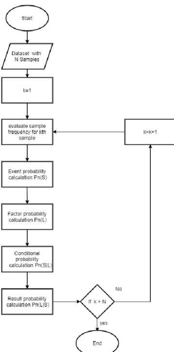
In order to apply this concept to the dataset, firstly; dataset classes should be visible and clearly identifies. The class frequency means evaluating the number of times that every class is generated. So, the classes frequency table is the first important step in Naïve Bayes algorithm, the same is illustrated in the Fig 3.2 [35].

the second step in the Naïve bayes algorithm is the abstraction of the frequency table by evaluating the conditional probability, event probability, and the factor probability.

Pseudo Code Algorithm 1: Pseudo code of Naive Bayes

/* Generating class probability P (m) (Training)*/ /*M Number of classes */

/* x data input*/

1: 𝑰𝒏𝒑𝒖𝒕 𝒅𝒂𝒕𝒂 x, Number of classes M; /*input dataset, create classes */ 2: 𝐟𝐨𝐫 𝑖 = 1: 𝑀 𝐝𝐨:

3: 𝐥𝐨𝐠 − 𝐩𝐫𝐢𝐨𝐫 (𝒎) = 𝒍𝒐𝒈 (𝒏𝒖𝒎𝒃𝒆𝒓 𝒐𝒇 𝒆𝒍𝒆𝒎𝒆𝒏𝒕𝒔 𝒊𝒏 𝒄𝒍𝒂𝒔𝒔𝒆𝒔 / 𝒏𝒖𝒎𝒃𝒆𝒓 𝒐𝒇 𝒆𝒍𝒆𝒎𝒆𝒏𝒕𝒔 𝒊𝒏 𝒙 )

4: 𝐞𝐧𝐝 𝐟𝐨𝐫

5: /* calculation of P (element\m). e: number of elements (Test)*/

6: 𝐟𝐨𝐫 𝑖 = 1: 𝑒 𝐝𝐨:

7: 𝐩 (𝐞\𝐦) = 𝐥𝐨𝐠 [(𝐩(𝐞(𝐢), 𝐦) + 𝟏)/(𝐒𝐔𝐌(𝐩(𝐞, 𝐦) + 𝟏))] 8: 𝒓𝒆𝒕𝒖𝒓𝒏 𝑷(𝒆\𝒎), 𝑷(𝒆, 𝒎), 𝒆

9:𝐞𝐧𝐝 𝐟𝐨𝐫 10: 𝑬𝑵𝑫

Figure 3.2. Naive Bayes Algorithm flow diagram.

3.3.2. K Nearest Neighbour Algorithm

K Nearest Neighbour (or K-NN) is one of the machine learning algorithms, it is classified under the supervised machine learning algorithms. This algorithm is popular by its simplicity and it required no parametrical evaluation and no likelihood calculations. The k Nearest Neighbour Algorithm can be work using three major steps of action [36].

Determination of number k is important. k has to be positive integer number. It represents number of considered neighbours. For a known dataset, preprocessing of the data is must be done at the beginning. Then k-NN process can be split into three main steps:

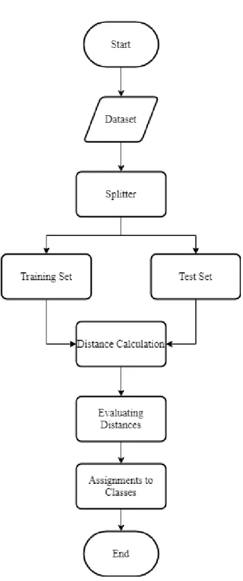
1. Evaluation of the distance. Distances are calculated between test data and training data. Most common metrics for distance are Euclidian distance, Manhattan distance and Hamming distance. Euclidian is the most frequent one. 2. Identification of the nearest Neighbour according to the distance information.

Distances are sorted in ascending order. Then top k neighbours are preferred. 3. According to the nearest Neighbours, the results that represent the prediction are

made. Top k number of distances are chosen from sorted list and a point is assigned a class to the test point depend on most frequent class of the list.

The Euclidean distance between two points can be calculated using the equation (3.3).

𝑑(𝒙, 𝒙

) = √(𝑥

− 𝑥′

)

_{+ (𝑥}

2

− 𝑥′

)

Where d represents distance between element of test data x and each training element x'. As the Euclidean distance is being evaluated for each element, the classes are now ready for graphical representation as demonstrated in Figure 3.3 illustrates three types of classes in the graph and each class is far from a particular Euclidean distance from the other. each class is represented by using specific color as circle, yellow, blue and green.

Figure 3.3. Graphical representation of three different classes [37].

The second action to be taken by the K Nearest Neighbour algorithm is to evaluate the nearest distance between the classes.

The distance values are sorted in ascending order and top k numbers of distance are selected.

The last step in the K Nearest Neighbour algorithm is to perform the classification. However, the classification is to be made based on frequency of the nearest k neighbour's classes of training dataset. The class of the test data is assigned according to most frequent class in the nearest k neighbours.

The similarity of the distance will lead to a decision that this entry of the test set is related to the class with the best similarity. Figure 3.4 demonstrates the process of the K Nearest Neighbor algorithm from the beginning until making the decision.

Pseudo Code Algorithm 2: Thyroid detection using KNN

/*X: Training data, Y: Known classes for X, x: Sample from test data*/ /* d: Distance between class and sample*/

/* M: Number of elements in X, N: Number of elements in test set*/ /* K number of nearst neighbor*/

1: 𝑰𝒏𝒑𝒖𝒕 𝒅𝒂𝒕𝒂 x, X, Y; 2: 𝐟𝐨𝐫 𝑖 = 1: 𝑁 𝐝𝐨: 3: 𝐟𝐨𝐫 𝐣 = 1: 𝑀 𝐝𝐨: 4: Calculate distance: d(Xj, xi) 5: 𝐞𝐧𝐝 𝐟𝐨𝐫

6: sort distances in ascending order

7: Assign xi to most frequent class in the k nearest neihbours.

8: 𝐞𝐧𝐝 𝐟𝐨𝐫 9: 𝑬𝑵𝑫

3.3.3. Random Forest Algorithm

In 2001, Bierman had proposed the so-called random forest algorithm that performs clustering, classification, and forecasting (prediction). In the literature, plenty of works has been done in order to enhance the performance of the random forest algorithm so that it yields reliable accuracy of prediction/clustering and it can tolerate more abnormalities in the data such as noise and missing values. Noise tolerance in an algorithm is termed to the level of noise that the algorithm can produce its results with required accuracy [38].

Random forest bootstrap is a process performed by this algorithm for extracting the elements (samples) from the original samples in order to form the so-called tree. The tree itself has its own restriction to form the branches which are termed to the classes/clusters of the data.

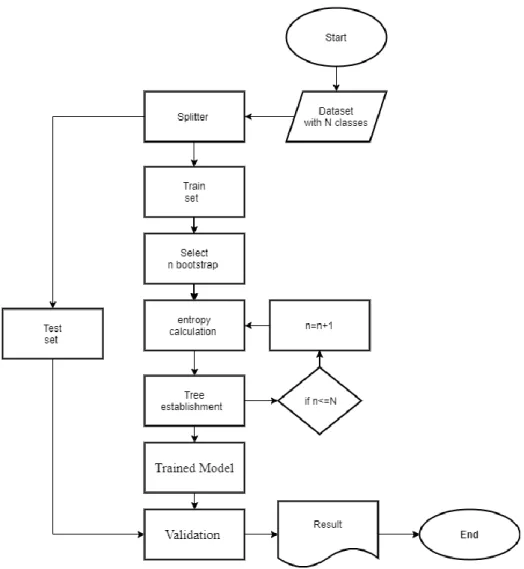
Figure 3.5. Random Forest algorithm flow diagram.

Random forest is performing the classification tasks as following steps:

1. Collecting the dataset values as it has resulted from the preprocessing phase and performing the first step of action called bootstrapping, which involves collecting the class (branch wise) samples from the main data.

2. For each collected sample, the entropy calculation might be initiated in order to determine the amount of correlation between the selected sample and the specific branch.

3. The term forest is allotted for class trees that contained multiple trees. For each bootstrap sample, M decision trees are formed which is called a training phase of the random forest.

4. The training of each decision tree is independently taking place by rearranging the samples of the data in each tree. Every time, rearranging of data sample in the tree, entropy measure can be made for detecting the enter class correlation. 5. Performance of classification in the random forest algorithm can be measured

using standard performance metrics such as accuracy, mean square error, and mean absolute error.

Pseudo Code Algorithm 3: Thyroid detection using Random Forest

3.3.4. Long Short-Term Memory Neural Network (LSTM)

LSTM neural network is a popular type of neural network that depends on a backpropagation training mechanism. LSTM is basically constructed as a recurrent neural network, the prediction of the data in a recurrent neural network is depending on the previous information of the same data. For example, prediction of the next word in the speech sequence (sentence) using the recurrent neural network is depending on the previous word in the same sequence[10].

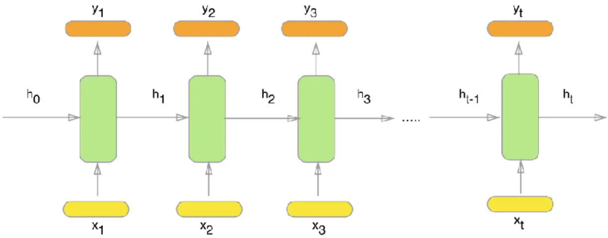
Figure 3.6. Recurrent neural network structure.

Assuming the demonstration given in Figure (3.6) above, a prediction of the next word in a spoken sentence contained (t) number of words. Each word is represented as x1, x2, xt as shown in the figure. The input words are feed into (t) number of training models (such as the individual neural network) each neural network will be trained individually on the provided input and will produce the output as y1, y2, y3, yt. In the recurrent neural network, the next output prediction is depending on the previous output from the previous neural network which is updating the next model training procedure by producing coefficients alike h1, h2, h3, ht. Where J is the cross entropy in Eq. 3.4.

ℎ

𝑦

= 𝑠𝑜𝑓𝑡𝑚𝑎𝑥(𝑤

ℎ

)

𝑗

(𝜃) = ∑

( 𝑦

𝑙𝑜𝑔 𝑦

Getting the required accuracy from the recurrent neural network is not as easy. The problem is the vanishing gradient problem which is acts against the accuracy of training. The problem solved by the modern type of recurrent neural network named LSTM neural network which designed to combat vanishing gradient through a gating mechanism as illustrated in Fig (3.7).

Figure 3.7. LSTM neural network internal structure (gate unite)[10]

LSTM consist of three gates and cell memory: -

1. Input gate: determine what part of the current vector matter.

𝐶`_𝑡 = 𝑎𝑡^ = tanh(𝑊_𝐶. 𝑋𝑡+ 𝑈_𝑐 . ℎ𝑡−1+ 𝑏𝑐 ) = tanh(â 𝑡) (3.5)

𝐼𝑡 = σ(𝑊𝑖. 𝑋𝑡+ 𝑈𝑖 . ℎ𝑡−1+ 𝑏𝑖 ) = σ(Î𝑡) (3.6)

2. Forget gate: determine whether the past should be forgeted or preserved.

𝑓_𝑡 = σ(𝑊_𝑓. 𝑋𝑡_{+ 𝑈}

𝑓 . ℎ𝑡−1+ 𝑏𝑓 ) = σ(𝑓^𝑡) (3.7)

3. Output gate: determine what data should be output to the h of the current should be forgeted or preserve hidden stat or preserved in the cell stat.

𝑂_𝑡= σ(𝑊_𝑜. 𝑋𝑡_{+ 𝑈}

𝑜 . ℎ𝑡−1+ 𝑏𝑜 ) = σ(Ô 𝑡) (3.8)

4. Memory cell output:

5. Hidden layer output:

ℎ𝑡 = 𝑜𝑡⊙ tanh(𝐶𝑡) (3.10)

So we can simplify the entire computation in the Matrix form as:

𝑍𝑡 = | â 𝑡 Î𝑡 𝑓^𝑡 Ô 𝑡 | = | 𝑊𝑐 𝑈𝑐 𝑏𝑐 𝑊𝑖 𝑈𝑖 𝑏𝑖 𝑊𝑓 𝑈𝑓 𝑏𝑓 𝑊𝑜 𝑈𝑜 𝑏𝑜 | × | 𝑋𝑡 ℎ𝑡−1 1 | (3.11)

Where w is weight of the current input and U is the weight of the input from previous hidden layer and b is a biase.

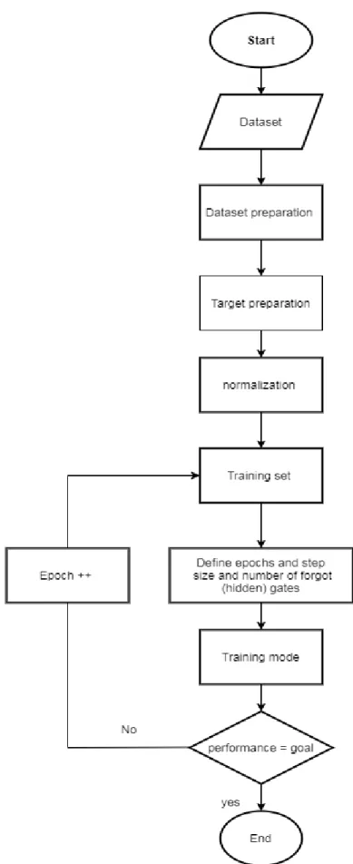
LSTM memory neural network is designed to tackle the learning error and training malfunctioning especially when the data is of varying nature. The model is beginning with defining the inputs array which is the data (training set) and the target array. However, in LSTM neural networks, there is no requirement to define the data in such format alike horizontal or vertical representation as to the situation with a classical feed-forward neural network; data can enter in normal rows and columns and the target can be normal row or column represented array.

The disputed point is to identify the number of hidden layers that are impacting the entire performance of the model. In our work, we tried using different numbers of hidden gates to meet the various requirements in the performance such as too downscale the time or to uplift the accuracy. We land up with two hidden gates, which provided us with both time and accuracy requirements.

The model is set ultimately to intake the data of two thousand cases and perform the training to map the test data hereinafter for the appropriate decision in the target array. Furthermore, a value normalization implemented in the input stage of the long short term memory neural network.

Data normalization is made to scale down the value of the cell to be a crack of one and however, Normalization integration of the input stage is one of the approaches that made from meeting the higher accuracy[27]. The LSTM model, then beginning the training process after defining the required parameters such as the patch size and the epoch number and by defining the performance metric parameter which is made as an accurate measure in this study. The Fig 3.8: demonstrating the model stages in a graphical flow diagram.

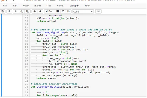
3.3.5. K-fold Cross Validation

K-Fold Cross Valdiation is a resampling procedure used to evaluate machine learning models on a limited data, in order to verfy the classfier performance of different combinations of the input data of both training set and testing set k-fold cross validation is used where a given data set is split into a K number of folds.

K is representing the number of folds which is corresponding to the number of input data of both train and test sets When a specific value for k is chosen, it may be used in place of k in the reference to the model, such as k=10 becoming 10-fold cross-validation. That means the data set is split into 10 folds. In the first iteration, the first fold is used to test the model and the rest are used to train the model. In the second iteration, 2nd fold is used as the testing set while the rest serve as the training set. This process is repeated until each fold of the 10 folds have been used as the testing set [38].

In our work we used cross valdition to evaluate to random forest algorithm to get perfect performance and part of code shown in Fig. 3.9.

PART 4

APPLICATION

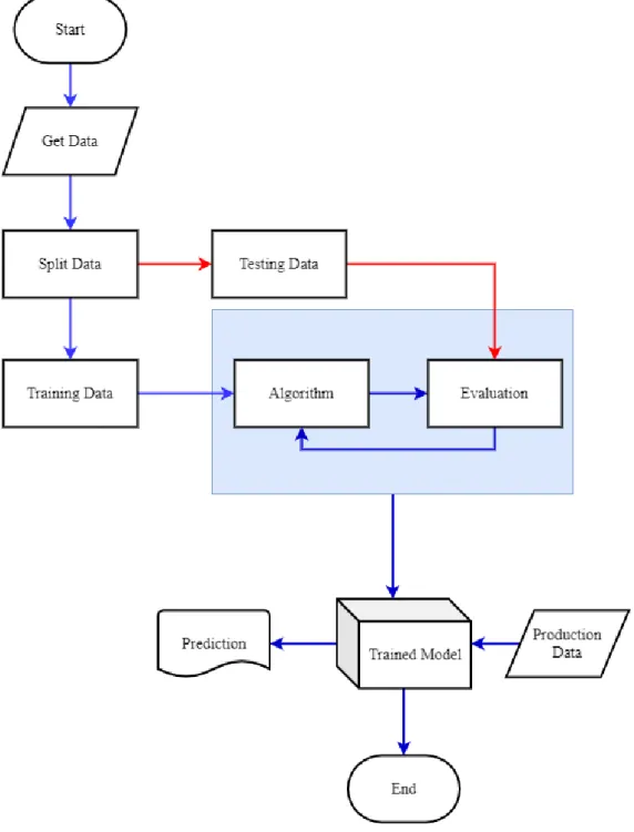
In this section, all steps of classification methods are presented. Python and its libraries: Sci-Kit, Numpy and Keras were used for programming and Jupyter Notebook on Anaconda was preferred as development environment. The general flow of the study is given in Figure 4.1.

The data were taken from UCI Machine Learning repository. The missing values of the dataset were completed with mean value. Then dataset was splitted into two groups as training and testing. After that, the machine learning algorithms were applied (trained). Finally, classifier model (the blue box) seen in Figure 4.1 is obtained. The blue box is final product of the algoritms. A new patient’s testing results can be given to the blue box and it will classify the patience’s situation.

4.1. PRE-PROCESSING

Dataset was downloaded from the repository and organized. All the 2800 records are being diagnosed in the hospital by specialist doctors and the decisions of diagnoses are made as in Table 4.1. This column is an important part of the dataset which represents the target and will be essentially used while mining the data. The classes realized in the target are four, namely: negative, hyperthyroid, T3 toxic, and goiter.

Table 4.1. Target encoding and class description.

Diagnosis Class code

Negative 0

Hyperthyroid 1

T3 toxic 2

Goiter 3

The data encoding in this section is having the objective to convert the data into numbers where the gradience between the cells will be minimized and hence the performance of training will be increase. For true/false values encoding is done with logical 0 and 1 as seen in Table 4.2.

Table 4.2. Dataset cells encoding and conditions. Cell value (condition) Code

If cell value is “male” Return 0

If cell value is “female” Return 1 If cell value is “true” or is “t” Return 1 If cell value is “false” or is “f” Return 0

If cell value is “p” Return 1

If cell value is “N” Return 0

One of the most important steps in this process is ignoring the columns that not having any impact in decision making, such as patient’s name, address or any other similar information. Such information might increase the load on the machine without any benefit in decision making.

The other step in pre-processing is the condition awareness which implies what is the suitable value to be replaced in place of the cell in order to convert it into a logical format. Table (4. 2) is demonstrating the condition of all the columns.

The missing values occur in most of the public datasets and it resulted due to various factors such as damaging the data storage devices and hence the backup process may fail to recover all the data in the same original accuracy.

Another factor can be the time factor, more specifically, the medical data can be collected by referring to the medical investigations for the last ten years of the patient group. However, those recorders are likely to be paper records spatially when we talk about data established in the mid-90s. Those paper records might get scratches and damages, so the visibility of particular information might be impossible, hence it is entered as a null or missing record.

Many techniques found feasible in the literature to tackle the drawbacks of missing values. Such drawbacks are related to the training performance when we treat the data under a smart machine learning paradigm. The missing values may throw an error

while training. Hence, recovering or replacement of missing data is a demandable approach.

One of the feasible methods to replace the missing values is called a mean values method [27]. It basically determines the average of the column (the particular data field where missing values are reported). This method is made to reduce the variance between the columns values by replacing the missing value with the average number of all column values.

Another important thing which applied to data is a normalization method which is a preprocessing technique used to rescale attributes values to fit in a specific range, we use a method called (min – max normalization value) which can be calculated using the Equation 4.1 [39].

𝑉` = 𝑣 − 𝑚𝑖𝑛

𝑚𝑎𝑥 − 𝑚𝑖𝑛 (4.1)

Where V` is the normalized value, v is th original value, min is the minimum and max is the maximum value in a given data.

After the data preprocessed and normalized, it was executed by each algorithm mentioned in the above section. The data set is splitting into two groups training set and testing set. This is one of the crucial steps to evaluate the real performance of our models. We applied 70% of data set for training and 30% of data set for testing within each model, and results are being evaluated.

4.2. APPLIED ALGORITHMS

4.2.1. Naïve Bayes Algorithm

For the thesis, Naïve Bayes algoritm was implemented in Python. In Figure 4.2 development environment and part of the code is shown.

Figure 4.2. Implemented Naïve Bayes algorithm.

We run the algorithm ten times, in each run evaluation metric values were different because training and test data selected randomly. The mean values of performance metrics are accuracy: 21.072, mean absolute error: 10.527, mean square error: 7.121 and duration: 0.165 seconds.

4.2.2. K Nearest Neighbour Algorithm

For the thesis, k-NN algoritm was implemented in Python. In Figure 4.3 development environment and part of the code is shown.

4.2.3. Random Forest Algorithm

For the thesis, random forest algoritm was implemented in Python. In Figure 4.4 development environment and part of the code is shown.

Figure 4.4. Implemented random forest algorithm.

We tried different max depth values for trees and the best performance was obtained with 5. The best performance metric values are accuracy: 97.10, mean absolute error: 0.04, mean square error: 0.04 and duration: 116.59 seconds.

4.2.4. Long-Short Term Memory Neural Network

We used keras library for LSTM algorithm. Figure 4.5 shows development environment. We obtained the best performance metrics at 20 epochs. Model accuracy and loss function graphics are shown in Figure 4.6 and 4.7 respectively. Performance metrics are loss: 0.0543, accuracy: 0.9725 for training and loss: 0.0543, accuracy: 0.9725 for validation with test data.

Figure 4.6. Model accuracy graphics.

PART 5

RESULTS AND DISCUSSION

5.1. PREFACE

The thyroid dataset is being applied for processing on the Naïve Bayes algorithm, K Nearest Neighbour algorithm, Random Forest Algorithm. On the other hand, a deep learning approach is used to evaluate the performance of a high-level algorithm. LSTM neural network is being used for performing the same prediction task.

5.2. ACCURACY OF PREDICTION

In this section, the accuracy of prediction in each algorithm is measured in order to evaluate the number of the percentage of correctly predicted results to the total number of results. The accuracy of the prediction of the disease is given in equation 5.1.

𝐴𝐶 = 𝐶𝑃

𝑇𝑃∗ 100% (5.1)

Where Cp is the number of correct decisions and Tp is the number of the total decisions including the correct and incorrect decisions, finally, AC is the percentage of the accuracy measure calculated for the output results.

Table 5.1. Accuracy measure in the tools used in this project.

Tool Accuracy (%)

KNN 71.20

N. Bayes 21.072

RF 97.10

Table 5.1 is represented graphically in Figure 5.1. however, the Figure illustrates the accuracy of the results in the LSTM neural network is found to be the best accuracy level. Whereas the minimum accuracy percentage is found in the Naïve Bayes algorithm. The accuracy of the random forest Algorithm is found second-best accuracy after the LSTM neural network.

Figure 5.1. Graphical representation of the accuracy measure in the tools used in this project.

5.3. TIME OF PREDICTION

Another performance metric is being determined for each algorithm; the time is an important factor of the success of any processing tool. It is vital to the success of any applications alike the real-time applications and live broadcasting. The first three algorithms that made to predict the disease from the thyroid dataset (among the Machine Learning algorithms).

The time delay that calculated from the beginning of the algorithm until the end of the program and display and the results are being observed. The maximum time is realized taken by the Random Forest algorithm and the minimum time is seen produced by the K Nearest Neighbour algorithm.

On the other hand, the Long Short Term Memory Neural Network is seen moderated if the high accuracy is considered. The time taken by the deep learning tools (LSTM neural network) can be said as moderated as compared to the other algorithms which produce lesser accuracy. Table 5.2 is demonstrating the time in seconds calculated for each algorithm. However, Figure 5.2 is depicting the time graphically and showing the fluctuation in time amongst the algorithms.

Table 5.2. Time measure in the tools used in this project.

Tool Time (seconds)

KNN 0.11

N. Bayes 0.165

RF 116.59

LSTM 0.210

Figure 5.2. Graphical representation of the Time measure in the tools used in this project.

5.4. MEAN SQUARE ERROR OF THE PREDICTIONS

This performance metric is an important factor to judge the performance of Machine learning and Deep Learning paradigms. The mean square error is revealing about the amount of error in the results. In another word the mean square error and root mean

square error is abstracting the error amount in the results. Table 5.3 and Figure 5.3 are demonstrating the mean square error in both numerical and graphical representations. The Long short term memory neural network is seen with the second minimum mean Absolut error after the random forest algorithm.

Table 5.3. MSE measure in the tools used in.

Tool MSE

KNN 2.00

N. Bayes 7.121

RF 0.04

LSTM 0.0601

Figure 5.3. Graphical representation of the MSE measure in the tools used in this project.

5.5. MEAN ABSOLUTE ERROR OF THE PREDICTIONS

The mean absolute error is another performance metric which made to provide more abstraction to the error amount in the result. The difference between the mean square error and mean absolute error is that mean absolute error is providing more abstraction of the error by reducing the values of the metric. Table 5.4 and Figure 5.4 are

demonstrating the mean square error in both numerical and graphical representations. LSTM neural network is seen with the minimum mean Absolut error after Random Forest Algorithm.

Table 5.4. MAE measure in the tools used in this project.

Tool MAE

KNN 1.274

N. Bayes 12.413

RF 0.039

LSTM 0.0601

Figure 5.4. Graphical representation of the MAE measure in the tools used in this project.

5.5. ROOT MEAN ABSOLUTE ERROR OF THE PREDICTIONS

Root mean square error is an important factor of a performance metric to judge the performance of the between the Machine learning and Deep Learning paradigms. The root mean square error is revealing about the amount of error in the results. Root mean square error is made to generate more readable (smaller values) of the root mean square error. Table 5.5 and Figure 5.5 are demonstrating the root mean square error in both numerical and graphical representation.

Table 5.5. RMSE measure in the tools used in this project. Tool RMSE KNN 1.413 N. Bayes 3.102 RF 0.197 LSTM 0.245

Figure 5.5. Graphical representation of the RMSE measure in the tools used in this project.

Table 5.6. Performance metrics results of all algorithms used in the study.

Metric

AlGO

Accuracy Time MSE MAE

KNN _71.088 0.360 1.997 1.274

N. Bayes

36.071 0.435 9.627 12.413

RF _96.7 487.73 0.039 0.039

Looking at the results shown in Table (5.6), the following can be observed:

The accuracy obtained from LSTM was high due to the fact that it works to reduce overfitting and its internal structure, which contains three gates and cell memory, which work together as a single unite makes it give high accuracy.

Also, RF gives a high accuracy rate, even less than LSTM, because of its handling of the data, as it divides main data into samples and each sample into multiple trees, which reduces the risk of overfitting as well as estimates missing data cause high accuracy.

Also, N. bayes gives a law accuracy because it depends on it’s work on probabilities so if a categorical variable has a category in the test set which not observed in training dataset the model will assign zero probability and will unable to make a prediction this often knows as (zero frequency)[40].

In the time performance matrix, we find that the RF took a long time because it divides the data into samples and samples into a number of trees decision which makes the algorithm too slow, and longer time to train, but of course, the time depends on the specifications of the computer.