INFLATION MODELING
Sinan Bekar
111624002
SOSYAL BİLİMLER ENSTİTÜSÜ
FİNANSAL EKONOMİ / SAYISAL FİNANS
YÜKSEK LİSANS PROGRAMI
Yard. Doç. Dr. Haluk Yener
2015
3
ACKNOWLEDGMENTS
I would like to thank my thesis advisor Asst. Prof. Dr. Haluk Yener for his kindness and forbearance. I am really thankful for his tolerant guidance and encouragements. I am thankful for having the chance to work with him.
I also would like to thank my friend Fuat Can Beylunioğlu who help me on Eviews and R package program in this study.
Finally, I am so grateful to my family for their motivation during the thesis period and I am really indebted to my family for their endless support. They always encourage and support me in all my stressful times. Therefore, I am dedicating this thesis to my great family.
4
ÖZET
Bu tez, Haluk Yener’in 2006 yılında yaptığı Enflasyon Modellemesi yüksek lisans tezinin üzerine kurulmuş ve kendisinin literatüründen ve genel yaklaşımından faydalanılmıştır. Asıl amaç, gelişmekte olan ülke ekonomilerinin enflasyon tahmini için tasarlanan ve Gürcistan’ın enflasyon modellemesi için kullanılan Maliszewski Denkleminin, son yıllarda istikrarlı bir ekonomiye sahip olan Türkiye Cumhuriyeti’nin enflasyon tahmini için, bir teorik model olarak ateorik modellere kıyasla performansını yeniden test etmektir. Daha önceden yapmış olduğu çalışmasında, Yener (2006) ateorik modeller olan AR(2) ve TAR modellere kıyasla, Maliszewski Denkleminin 1988-2006 yılları arasında daha iyi bir performansa sahip olduğunu göstermiştir. Ancak, bu tezde 1999-2013 yılları arasında yaptığımız çalışmada, Maliszewski, diğer iki ateorik modele göre daha kötü bir performans göstermiştir. Bulgulardaki bu farklılığın nedenlerinden bir tanesini Türkiye’nin son on senedeki isktikrarlı ekonomik yapsını gösterebiliriz.
ABSTRACT
This thesis is built on Haluk Yener’s (2006) master thesis which is called Inflation Modelling and benefited from his literature and general framework1. Main purpose is to test again Maliszewski Equation, previously developed for estimating emergent market economies’ inflation and was also applied to Georgia’s inflation, for Turkey’s inflation forecast which has stabile economic structure in recent years, as a theoretical model for comparing with atheoretical models. The previous study by Yener (2006) found that Maliszewski Equation had the best performance when compared to the atheoretical models AR(2) and TAR through the observation period of 1988-2006. However, in this study, we found that it has worst performance in comparison with AR (2) and TAR model within the observation period of 1999-2013. As one of the main reasons that changed the previous results, we may suggest Turkey’ stabile economic structure in the last decade.
5 TABLE OF CONTENTS ÖZET ... 4 ABSTRACT ... 4 ILLUSTRATIONS ... 5 1) INTRODUCTION ... 7
2) GENERAL FRAMEWORK AND COMMON APPROACH ... 7
2.1) Definition of Variables ... 7
2.2) Description of Models and Model Selection Methods ... 7
2.2.1) Description of Models ... 8
2.2.2) Model Selection Methods ... 12
3) LITERATURE REVIEW ... 12
4) ESTIMATION AND FORECASTING STUDY ... 18
4.1) Maliszewski’s Equation for Inflation Forecast ... 19
4.2) Data ... 21
4.3) Estimation Methodology and Results ... 22
4.3.1) Maliszewski’s Equation ... 22 4.3.2) ARMA(p,q) Model ... 31 4.3.3) ARMA (3,2) Model ... 32 4.3.4) AR (2) Model ... 34 4.3.5) TAR Model ... 38 4.3.6) Forecast Results ... 43 5) CONCLUSION ... 44 6) REFERENCES ... 45 7) APPENDICES ... 47
7.1) Appendix A: ADF Tests on Variables ... 47
7.2) Appendix B: Maliszewski’s Equation Results ... 51
7.3) Appendix C: Diagnostic Test Results for the Maliszewski’s Equation ... 52
7.4) Appendix D: AR (2) Model and Diagnostic Test Results ... 55
7.5) Appendix E: TAR(2) Model and Diagnostic Test Results ... 59
6
ILLUSTRATIONS
Figure 1: Plots of Time Series ▪21
Figure 2: Quarterly Path of Turkish Inflation ▪24 Figure 3: Plot of Errors ▪25
Figure 4: Histogram for Normality ▪27 Figure 5: Plot of Recursive Residuals▪28 Figure 6: Plot of Cumulative Sum ▪28
Figure 7: Plot of Cumulative Sum of Squares ▪28 Figure 8: One-Step Probabilities ▪29
Figure 9: N-Step Probabilities ▪29 Figure 10: Recursive Coefficients ▪30 Figure 11: Correlogram of Log Pt ▪31 Figure 12: Plot of Recursive Residuals▪35 Figure 13: Cumulative Sum of AR(2) Model ▪35 Figure 14: Cumulative Sum of Squares of AR(2) ▪35 Figure 15: One Step Probability Plot of AR(2) ▪36 Figure 16: N Step Probability Plot of AR(2) ▪36 Figure 17: Recursive Coefficients Plot of AR(2) ▪37 Figure 18: Δ log Pt Plot with Threshold ▪39
Figure 19: Plot of Recursive Residuals – TAR(2) ▪40 Figure 20: Cumulative Sum of TAR (2) ▪41
Figure 21: Cumulative Sum of Squares TAR(2)▪41 Figure 22: One Step Probability Plot of TAR(2) ▪41 Figure 23: N Step Probability Plot of TAR(2)▪41 Figure 24: Recursive Coefficients Plot of TAR(2 ▪42
Figure 25: Correlogram on ARMA (3,2) Model Residuals ▪55 Figure 26: Correlogram of TAR(2) Model Residuals ▪60 Figure 27: Forecast of AR(2) Model ▪61
Figure 28: Forecast of TAR(2) Model ▪61
7
1) INTRODUCTION
The number of inflation forecast models in the literature is exhaustive as inflation is an important instrument for government politics, economic stability and future economic decisions, etc. Therefore, this thesis first reviews many inflation studies which include inflation modeling and forecasts. In addition to these, its purpose is to forecast inflation in Turkey via the application of theoretical and atheoretical econometric models. To this end, this thesis compares the inflation forecasts of Turkey obtained by the use of Maliszewski’s Model with the use of other two atheoretical time series models which are namely AR(p) and TAR models. As we will explain more thoroughly in the following sections, Maliszewski Equation (2003) was first developed by Wojciech Maliszewski to estimate emergent market economies’ inflation and it was also used for Georgia’s inflation modeling2.
2) GENERAL FRAMEWORK AND COMMON APPROACH
Inflation is defined as a sustained increase in the aggregate or general price level in an economy. In other words, inflation means that there is an increase in the cost of living. Therefore, forecasting inflation is a very important issue for future investment and saving decisions. Hence, econometricians or economists who try to estimate inflation and according to structure of economics, generally use three models to forecast inflation. These are respectively, atheoretical linear or non-linear time series models, structural models based on an economic theory, and surveys that measure the expectations of agents in an economy.
2.1) Definition of Variables
Generally, the change in the price level is obtained using Consumer Price Index (CPI). Therefore, the change in CPI is used as a dependent variable to measure inflation. On the other hand, the independent variables that we use to forecast inflation may be categorized under three types: First one are the nonfinancial macro indicators which are mainly consumption, investment, unemployment rates, money supply etc. Second are the financial variables which are interest rates, default spreads, exchange rates, etc. Finally, a third type are the surveys of inflation expectations which are obtained from opinions of professional forecasters, households and firms. As a result, according to structure of economy, there are a lot of options to predict inflation and in the thesis when constructing the theoretical model we benefit from financial and non-financial variables to forecast inflation which is defined as the quarterly percentage change in CPI.
2 Wojciech Maliszewski (2003), “Modeling Inflation in Georgia” Applied Economics. April, 2009, Vol. 41 Issue 10, p1203, 11 p.
8
2.2) Description of Models and Model Selection Methods
2.2.1) Description of Models3
The theoretical models generally have been improved with non-stochastic mathematical entities and have been implemented via the use of the empirical data and the addition of a stochastic error to the mathematical model4. In short, the model is formed between inflation and economic indicators through their causality relationships. However, such procedure may have its own disadvantages as the causality may be spurious. That is, as Granger and Newbold (1974) showed, there may be a spurious relationship between two unrelated variables with random walk pattern5. The main purpose of the study was to destroy stochastic trends in the time series, because stochastic trends cause non-stationarity in economic time series. In an earlier study, Box and Jenkins (1970) proved that the trend could be suspended with differencing the time series. Therefore, when the trend is taken away with first differencing, variable becomes I(1) stationary. Hence, Augmented Dickey Fuller (ADF) test, which is found by Dickey and Fuller in 1979, or series of other tests are used to test the variable for stationarity. In general, many economic series are found to be I(1). That is, many of them include stochastic trend and may be converted to stationary variables with first differencing.
Furthermore, Box and Jenkins method also introduced the error correction models (ECMs)6. Mainly thanks to ECMs, the autoregressive distributive lag (ARDL) models could be written in the error-correction form. In summary, we eliminate spurious relations from structural model with ECM and cointegration estimation as we know from Engle and Granger (1987) that variables of models built under ECM approach were also said to cointegrate. Box and Jenkins’s approach led to the birth of new models for the time series. These are mainly called ARIMA (Auto Regressive Integrated Moving Average) time series. When applying them for forecasting inflation we observe that ARIMA models consider the forecasted inflation as a function of its past values, which are also called lagged variables. Therefore, we can say that these models aim to capture the memory in a time series and may also be useful
3 The mathematical interpretation of models may be found at the end of this section.
4 Katrina Juselius (2002), “Model and relations in economics and econometrics, ”Macroeconomics and the real world: Econometric Techniques and Macroeconomics, Volume1.
5 Ron P. Smith (2002), “Unit Roots and all that: the impact of time-series methods on macroeconomics,” Macroeconomics and the real world: Econometric Techniques and Macroeconomics, Volume1.
6 Katrina Juselius (2002), “Model and relations in economics and econometrics, ”Macroeconomics and the real world: Econometric Techniques and Macroeconomics, Volume1.
9
for short term forecasting. However, in optimal forecasts, the estimation may diverge as the time horizon becomes more distant. Apparently, the divergence impedes the predicting ability of the model. A method to address the problem is then to take into consideration the effect of other economic variables in inflation forecasting. In this case, we refer to VAR models since they are useful for measuring the simultaneous or joint relation of the historical variables. In addition, to understand the direction of the relation among the variables we may use Granger Causality Test (see Granger (1969)). In the VAR model, the time series characteristics of variables in terms of their lag lengths can be taken into consideration. In, this case, the model is expressed as VAR(p), where p gives the lag length. Once the VAR model is constructed, we may then use vector error-correction model (VECM) to control whether the results are due to spurious relation.
Although VAR and ARIMA may be used to forecast inflation, because they do not capture the non-linearity in data or uneven effect of serious economic shocks, they may yield poor results. Therefore, we may need to refer to other methods which capture structural breaks in the economy. These models are classified as regime switching models which are respectively Threshold Autoregressive Models (TAR), Smooth Threshold Autoregressive Models (STAR), Markov Switching Models and Neural Networks Models. Furthermore, besides linear and non-linear forecast models, combination of forecasting models are also used to forecast inflation. The combination may be the outcome of either only linear or non-linear models or both. In addition to econometric models, surveys are also used to estimate inflation and they include sample households, firms and professional forecaster’s inflation expectations. The Livingston Survey, The Survey of Professional Forecasters (SPF), the Michigan Survey, and European Commission’s Harmonized Consumer Survey are among the famous surveys for the inflation expectations. Generally, mean or median of the data are used to obtain survey results.
In short, we have many options to forecast inflation. According to economic structure, there are a lot of advantages or disadvantages for every model. Therefore, to decide which model is the best to forecast inflation is not a trivial task. As evident in what follows (see also Yener (2006)) finding an appropriate model for forecasting inflation even in atheoretical models is not easy as there are many to consider.
10
General ARMA Models
(example: ARMA(p, q))
q i i t i p i t i t i o t r a a r 1 1 where
p i i t ir 1 drive the AR process and
q i i t ia 1 drives the MA process.
VAR Model
(example: Bivariate case)
t t t t t t t t t t t t t t t t a r r a a r r r a r r r a r r r 1 0 2 1 1 , 2 1 , 1 22 21 12 11 20 10 2 1 , 2 22 1 , 1 21 20 2 1 1 , 2 12 1 , 1 11 10 1
where Φ is a n x n matrix, and {at} is a sequence of serially uncorrelated random vectors with mean zero and covariance matrix Σ.
TAR Model
(Example: two regime TAR model
with order (p1, p2), denoted by
TAR(p1, p2; d, r).) r Y if Y Y r Y if Y Y Y d t t p t p t d t t p t p t t 2 2 2 2 1 2 1 2 0 1 1 1 1 1 1 1 1 0 ... ... Where { i t
} for i=1, 2,.. is the innovation process with variances 12and 22.
d is the delay and r is the threshold parameters.
STAR Model t p i p i i t i d t i t i o t c x a s x F x c x
1 1 , 1 1 , 0 Where d is the delay parameter, Δ and s are parameters representing the location and scale of model transition, and F(.) is a smooth transition function. Usually F(.) is considered a logistic, exponential or a cumulative distribution function. Mainly STAR is a weighted linear combination of the below two models:
p i i t i i t p i i t i tx
c
c
x
c
1 , 1 , 0 1 0 2 1 , 0 0 1)
(
)
(
11 the F(.) function.
Markov-switching Model (Example: two-state Markov-switching model.)
2 1 2 1 , 2 2 1 1 , 1 1 t t p i i t i t t p i i t i t s if a x c s if a x c x The transition is driven by a hidden two-state Markov chain. st may take values in {1,2} and is a first order
Markov chain with probabilities:
P(st = 2| st-1 = 1) = w1 and P(st = 1| st-1 = 2) = w2
The innovational series {a1t} and {a2t} are sequences of i.i.d. random variables with mean zero and finite variance and are independent of each other. A small wi
means that the model tends to stay longer in state i, given that 1/ wi is the expected duration of the process
to stay in state i.
Artificial Neural Network Models
h t t i n i i t t
g
u
v
(
1')
1 1 ' 0 1
(a single layer ANN)where g(z) is the logistic function,
) 1 ( 1 ) ( z e z g .
When yt is modeled in levels then, yt+h = vthand
1 ... 1
t t p t y y . When yt is modeled in differences yt+h-yt = vthand
1 ... 1
t t p t y y .If we would like to use two layers then we obtain ANN with two layers in the below form:
h t t i n i ji n j j t t g g u v
( 1' ) 1 2 1 2 ' 0 1 2 12
2.2.2) Model Selection Methods
Deciding among the models lie in forecast evaluation. First, we need some statistical measures to ensure significance of explanatory variables, because we know from previous section that we expect to establish a relationship between inflation and other explanatory variables. Then, once an in-sample measure is established and the model is created, its out-of-sample performance should be measured7. As a result, root mean square error (RMSE) or mean square forecast error (MSFE) measures are used for the comparison. The application is done via the selection of a benchmark model, and if the ratio of the candidate model with the benchmark model is smaller than 1 and close to zero, then the candidate model is perceived to perform well. Additionally, we may also consider two further measures which may be taken as complementary to the aforementioned measure. These are mainly the forecast direction (M. Hashem Pesaran and Spyros Skouras 2002, McCracken and West 2002) and time distance criterion (Clive W.J. Granger, Yongil Jeon 2003). In forecast direction, as evident form its name, the capacity of the model to forecast the direction of the inflation is measured, while in the time distance the horizontal distance between the forecasted and the actual series is measured. We refer the reader to articles for further information.
3) LITERATURE REVIEW
In this section we review a number of studies that are relevant for this thesis. For an exhaustive review of the studies that are published until 2006 we refer the readers to Yener (2006). Here, we concentrate on studies that are published after 2006.
As we previously mentioned, inflation forecast studies rely on three types of models which are mainly theoretical models, atheoretical models and surveys of inflation expectations of businesses and households. Each approach is developed with the aim of increased robustness in forecasts. Nevertheless, there is still no conclusive evidence upon which approach consistently performs better than the other. Therefore, each still has its place in the literature and their performances rely upon the period and the country considered for a forecasting study.
7 Fisher, Jonas D. M., Chin Liu, and Ruilin Zhou (2002), “When can we forecast inflation?,” Economic
13
For example, in their atheoretical study, Sezgin and Çoker (2007) studied Turkish inflation forecast using Bayesian Vector Auto-regression (BVAR) models. In their study, they also compared BVAR models with Vector Autoregression (VAR) model in two different periods that are selected as January 1986 – December 2001 and January 1986 – December 2000. Within these periods seven different BVAR models are constructed, and then the forecast performances of these, for years 2002 and 2001 are compared with VAR model. Consequently, they found that the forecast performances of BVAR models are not better than VAR models for January 2002 – December 2002 period. The reason for this can be explained by the economic crisis happened at 2001. With this respect, another model is constructed for January 1986 - December 2000 period and the January 2001 - December 2001 forecasts are examined. Finally the results showed that, “BVAR models are much better than VAR models for estimating the real values of 2001”8.
By the application of similar technique Österholm (2008) investigated that whether the forecasting performance of Bayesian autoregressive and vector autoregressive models can be improved by incorporating prior beliefs on the steady state of the time series in the system. Therefore, he compared traditional methodology with the new framework—in which a mean-adjusted form of the models is employed—by estimating the models on Swedish inflation and interest rate data from 1980 to 2004. His results showed that the out-of-sample forecasting ability of the models is practically unchanged for inflation but significantly improved for the interest rate when informative prior distributions on the steady state are provided. Consequently, according to his study results, he said that “this new methodology could be useful since it allows us to sharpen our forecasts in the presence of potential pitfalls such as near unit root processes and structural breaks, in particular when relying on small samples”9.
The structure of the VAR models also help us to understand the pass-through effects of exchange rate changes on the domestic prices. Görmüş and Peker (2008) showed this effects in the Turkish Economy using vector autoregression (VAR) analysis. According to their empirical evidence, they said that “the exchange rate shocks explain about 72 percent of the forecast error variance of prices in the medium and long-term horizons. Therefore, the
8 Funda Sezgin, Elif Çoker (2007), “Analysing the Inflation in Turkey with Bayesian Vector Autoregression Models” , Marmara University Social Sciences Institute Journal, June 2007, Vol.7, p.287-300.
9 Par Österholm (2008), “Can Forecasting Performance be Improved by Considering the Steady State? An Application to Swedish Inflation and Interest Rate”, Journal of Forecasting, Jan.2008, Vol.27, p41-51. 11p.
14
exchange rate is an important source of forecast error variance in domestic inflation”10. Given this evidence, we account for the effect of the exchange rate to Turkish inflation by using the theoretical model of Maliszewski (2003).
In another pass-through study regarding the Turkish Economy, Akçağlayan and Civcir (2010) measured the monetary policy reaction functions of the Central Bank of Republic of Turkey (CBRT) over the periods 1987:01–2001:12 and 2002:01–2009:05. This study investigated how the monetary policy responded to the exchange rate shocks before and after adoption of inflation targeting regime and how large the effect of exchange rate shocks is accounted for in forecast error variances decompositions for monetary policy as compared to other shocks, using the VAR model. In the end, they showed that “there has been strong pass-through during whole period. Moreover, in the post crisis period, exchange rate has been the main reaction variable for the Central Bank of Republic of Turkey”11.
Thus, via VAR models we observe the effect of various macro variables on the Turkish Economy, especially on forecasting the Turkish inflation. In fact, (consider the relationship between the interest rate and inflation) Kaya (2013) investigated that the yield curve forecasting performance of Dynamic Nelson–Siegel Model (DNS), affine term structure VAR model (ATSM VAR) and principal component model in Turkey. He also investigated the role of macroeconomic variables in forecasting the yield curve. As a result, he reached very important results such as “Macroeconomic variables are very useful in forecasting the yield curve.” Second, “The forecasting performances of the models depend on the period under review.” Third, “considering the structural break which associates with change in monetary policy leads models to produce better forecasts than the random walk”.
While the abovementioned studies are examples for the application of VAR type models, we observe in the literature studies that rely upon the complex use of stochastic modelling. For example, Koop and Potter (2007) developed a new approach to change-point modeling which allows the number of changepoints in the observed sample to be unknown, assuming regime durations have a Poisson distribution. Their model approximately nests the two most common approaches: the time-varying parameter (TVP) model with a change-point every period and the change-point model with a small number of regimes. They focused on
10 Şakir Görmüş, Osman Peker (2008), “Inflationary Effects of Exchage Rate’s in Turkey” , Suleyman Demirel University The Journal of Faculty of Economics and Administrative Sciences, July 2008, Vol.13 No.2 p.187-202
11 Irfan Civcir, Anıl Akçağlayan (2010), “Inflation targeting and the exchange rate: Does it matter in Turkey?”
15
considerable attention on the construction of reasonable hierarchical priors both for regime durations and for the parameters that characterize each regime. A Markov chain Monte Carlo posterior sampler is constructed to estimate a version of their model which allows for change in conditional means and variances. As a result, they showed how real-time forecasting can be done in an efficient manner using sequential importance sampling. According to their study, they said that “their techniques were found to work well in an empirical exercise involving U.S. GDP growth and inflation. Empirical results suggested that the number of change-points were larger than previously estimated in these series and the implied model was similar to a TVP (with stochastic volatility) model”12.
Another alternative to VAR models is the use of Artificial Neural Networks for forecasting inflation. Erilli, Eğrioğlu, Yolcu, Aladağ, Uslu (2010) tried to check the predictions which have been obtained using the feed forward and recurrent Artificial Neural Network (ANN) for the Consumer Price Index (CPI). At the end of their study, they suggested that “new combined forecast has been proposed based on ANN in which the ANN model predictions employed in analysis were used as data”13. The reason for their suggestions is that they found some difference for July 2007, February 2008 and June 2008 between actual inflation value and forecasted inflation value in their model. As a result, they showed sensible reasons for these differences such as 2007 general domestic elections of Turkey, increasing prices of food and energy, persistently increasing oil prices and increasing electric and natural gas prices.
The above study is interesting as it suggests a combination of the forecasts. In another study as well, employed for the US inflation forecasts, the combination of the forecasts performed pretty accurately. Wright (2009) tried to forecast US inflation using Bayesian Model averaging. He said about his study that “I consider using Bayesian model averaging for pseudo out-of-sample prediction of US inflation, and find that it generally gives more accurate forecasts than simple equal-weighted averaging. This superior performance is consistent across subsamples and a number of inflation”14.
12Garry Koop, Simon M. Potter (2007), “Estimation and Forecasting in Models with Multiple Breaks” , Review
of Economic Studies, July 2007, Vol.74, Issue 3, p763-789, 27p.
13 N. Alp Erilli, Erol Eğrioğlu, Ufuk Yolcu, Ç. Hakan Aladağ, V. Rezan Uslu (2010), “Forecasting of Turkey
Inflation with Hybrid of Feed Forward and Reccurrent Artifical Neural Networks” Doğuş University Journal; Jan 2010, Vol.11, Issue 1, p42-55. 14p.
14 Jonathan H. Wright (2009), “Forecasting US Inflation by Bayesian Model Averaging” , Journal of
16
Furthermore, combination of theoretical and atheoretical models may provide accurate estimates as well because it helps reduce the forecast errors. Öğünç, Akdoğan, Başer, Gülenay Chadwick, Ertuğ, Hülagü, Kösem, Özmen, Tekatlı (2013) employed that univariate models, decomposition based approaches (both in frequency and time domain), a Phillips curve motivated time varying parameter model, a suite of VAR and Bayesian VAR models and dynamic factor models for producing short term forecasts for the inflation in Turkey. Eventually, they found that “the forecast combination leads to a reduction in forecast error compared to most of the models, although some of the individual models perform alike in certain horizons”15.
However, when forecasting inflation rather than taking combinations of country-wide forecasts, we may also consider province level inflation forecasts and use them to cope with the country-wide inflation. Tunay (2010) studied Turkey's province-based inflation using space-time autoregressive moving average (STARMA) models. Findings obtained from Tunay’s study showed that statistically significance level and explanatory power of model are both expressively high. Consequently, this model can be used for forecasting province-based inflation. Therefore, Tunay said that “political authorities can easily forecast inflation and thereby take necessary measures to cope with both province-based and country-wide inflation. As a result of these, success of executed policies will undoubtedly increase”16.
Another method, as we mentioned in the previous sections, is to use surveys. Şahinöz and Hülagü (2012) studied that inflation expectation errors to measure inflation uncertainty in Turkey by analyzing the Central Bank of Turkey Survey of Expectations data and investigates whether the disagreement among the survey participants can be used as a proxy for inflation uncertainty. They said that “disagreement seems to be a good proxy for inflation uncertainty for the 2001-2006 period while this relationship vanishes with the full-fledged inflation targeting regime after 2006”17.
In fact, more complex theoretical approaches may be used along with surveys. Mainly, Chernov and Mueller (2012) tried to estimate a factor hidden in the nominal yield curve using
15 Fethi Öğünç , Kurmaş Akdoğan, Selen Başer, Meltem Gülenay Chadwick, Dilara Ertuğ, Timur Hülagü, Sevim
Kösem, Mustafa Utku Özmen, Necati Tekatlı (2013), “Short-term inflation forecasting models for Turkey and a forecast combination analysis” , In Economic Modelling; July 2013, Vol. 33, p312, 14p.
16 K. Batu Tunay (2010), “Starma Modeling and Estimation of Province-Based Inflation in Turkey” , Hacettepe University Economics and Administrative Faculty Journal, Jan 2010, Vol.28 p.1-36
17 Timur Hülagü and Saygın Şahinöz (2012), “Is Disagreement a Good Proxy For Inflation Uncertaininty? Evidence from Turkey” , Central Bank of the Republic of Turkey, Central Bank Review; Jan 2012, Vol. 12, pp.53-62
17
information in the term structure of survey-based forecasts of inflation. Therefore, they constructed a model that accommodates forecasts over multiple horizons from multiple surveys and Treasury real and nominal yields by allowing for differences between risk-neutral, subjective, and objective probability measures. After that, they established that model-based inflation expectations are driven by inflation, output, and one latent factor. Consequently, they said that about their study and results. “We show that this hidden factor is not related to either current and past inflation or the standard set of macro variables studied in the literature. Consistent with the theoretical property of a hidden factor, our model outperforms a standard macro-finance model in its forecasting of inflation and yields”18.
Finally, recently, by using a different model than those aforementioned above, Monteforte and Moretti (2013) studied a mixed-frequency model for daily forecasts of euro area inflation. Their model combined a monthly index of core inflation with daily data from financial markets; estimates are carried out with the Mixed Data Sampling (MIDAS) regression approach. Thus, the forecasting ability of the model in real time is compared with that of standard VARs and of daily quotes of economic derivatives on euro area inflation. In sum, they find that “the inclusion of daily variables helps to reduce forecast errors with respect to models that consider only monthly variables. The mixed-frequency model also displays superior predictive performance with respect to forecasts solely based on economic derivatives”19.
As we saw different there are various different approaches that help to reduce the inflation forecast errors. Each seemed to perform relatively well depending on the objective, the period and the country under consideration. In fact, Clark and Doh (2014) reviewed alternative models for the concept of trend inflation and compared the models on the basis of their accuracies in out-of-sample forecasting, both point and density. In sum, according to their results, they said that seem to be about equally accurate, and the relative accuracy is somewhat prone to instabilities over time”20.
Neverthless, Rumler and Valderrama (2010) compared The New Keynesian Phillips Curve with time series models to forecast inflation. Therefore, they proposed a method of
18 Mikhail Chernov, Philippe Mueller (2012), “The term structure of inflation expectations” , Journal of
Financial Economics, Nov.2012, Vol.106, Issue 2, p367-394
19 Libero Monteforte, Gianluca Moretti (2013), “Real-Time Forecasts of Inflation: The Role of Financial
Variables” , Journal of Forecasting, Jan 2013, Vol.32, Issue 1, p51-61. 11p.
20 E. Todd Clark, Doh Taeyoung (2014), “Evaluating alternative models of trend inflation” , Internatiol Journal of Forecasting, July-Sept. 2014, Vol.30, Issue 3, p.426-448
18
forecasting inflation based on the present-value formulation of the hybrid New Keynesian Phillips Curve to evaluate the forecasting performance of this model using a Bayesian VAR, a conventional VAR and a simple autoregressive model. As a result, they concluded that “the New Keynesian Phillips Curve delivers relatively more accurate forecasts of inflation in Austria compared to the other models for longer forecast horizons (more than 3 months) while they are outperformed by the time series models only for the very short forecast horizon. This is consistent with the finding in the literature that structural models are able to outperform time series models only for longer horizons”21.
Given the above evidence, then, we seek to measure the relative performance of a theoretical model along with two atheoretical models, one capturing the linearity and the other one capturing the non-linearity in the data, for foreasting Turkish inflation. In this way, our aim is to understand whether a theoretical approach is appropriate for forecasting the inflation of an emerging country like Turkey or a simple atheoretical model would yield a better result. To this end, we move in the next section to describe the estimation and forecasting study.
4) ESTIMATION AND FORECASTING STUDY
What follows is outlined (straightforwardly in parts) from Maliszewski (2003) (see also Yener (2006)). For estimating and forecasting inflation, I used equation of Maliszewski (2003) and compared its performance with AR (p,q) and TAR model.
Wojciech Maliszewski made his model to forecast the Georgian inflation rate. The theory in the study is built upon the perception that prices increase with increasing money supply and depreciating exchange rate, and decrease with growth (i.e. GDP growth) in equilibrium and over the long run. Consequently, Maliszewski formulation is given by
p = α1/(α1+ α2)m + α2/(α1+ α2)e - 1/(α1+ α2)y,
where all the variables are in logarithmic form, and p is the consumer price index, m is the money supply, e is the exchange rate and y is the GDP.
21 Fabio Rumler, Maria Teresa Valderrama (2010), “Comparing the New Keynesian Phillips Curve with time series models to forecast inflation” , The North American Journal of Economics and Finance, August 2010, Vol.21, Issue 2, .126-144
19
We observe that the above equation depict the relationship between the price level and the relevant macro variables in emerging market economies. Therefore, the use of Maliszewski (2003)’s equation is intended to fill the gap which did not use these variables under structural models for predicting Turkish inflation.
4.1) Maliszewski’s Equation for Inflation Forecast
Long-term price level (P) behavior determined when there is a balance between the aggregate demand (YD) and supply (YS) of goods and services. The aggregate demand for goods and services is, in turn, considered as a function of real money supply (M/P) and the real exchange rate (E/P). From this, the aggregate demand is given in the log linear form by
yD = α1 (m – p) + α2 (e – p), (1)
where the above equality is in log linear form and lower case letters are used to denote the variables. The dame form and notation is used throughout this section.
The aggregate supply (AS) is given exogenously and in equilibrium is equal to aggregate demand and real income (Y):
y = yS = yD (2)
The above equality is obtained because Maliszewski (2003) assumed that the goods market is always in equilibrium.
Furthermore, following Maliszewski (2003) straightforwardly for the rest of this section, we write that the demand flow of foreign exchange is a function of real exchange rate and real income. Real income is at level with AS and is constant while real exchange tends to balance for foreign market currency. Money demand is supposed as a function of real income. Likewise, since real income is exogenous, real money balances tend to balance for the money market. If foreign exchange and money market are in equilibrium, the goods market is defined like equation (1) which is also in balance by application of the Walras law. If the market is in equilibrium, basic model defines 2 real variables (m-p and e-p) with one degree of freedom for determination of nominal variables (m,e and p). Fixing of the variables determines other two ones as providing a nominal power for the system. Empirically, if markets are in balance averagely, two special long run cointerating vectors probably occur between non-stationary nominal variables in equation (1) (treating y as exogenous). Moreover, money and foreign exchange markets may be permanently out of equilibrium (Adjustment is very slow or
non-20
linear in equilibrium). Only, according to the assumption, goods market is always in equilibrium. In this situation, fixing one of the nominal variables does not provide a nominal power anymore to the system but fixing of two ones determines third one in the equation (1). Empirically, if two market are out of equilibrium, only one cointerating vector can be found in the data as answering to equality in the equation (1). Permanent pressure of exchange rate may be an example disequilibrium type before Russian crisis. This inequality had influenced money market in the foreign exchange market. Therefore, it would cause unbalanced of money market. While equilibrium had been finally restored in the foreign exchange and money markets, the permanent of disequilibrium and a probably non-linear adjustment process may obstruct finding two cointegrating vectors among the series. Supposing that only goods market is in equilibrium, substituting (2) into (1) and solving for p gives the equilibrium price level.
p = α1/(α1+ α2)m + α2/(α1+ α2)e - 1/(α1+ α2)y (3)
Equation (3) is similar with price equation which developed by Bruno (1993) who describes a long term relationship between prices, exchange rate, money and real income. Even if money and real income are out of equilibrium, it is suitable for estimation and testing in the cointegration framework. This equation shows us a neo-classical dilemma and yS is fixed and equi-proportional changes in nominal variables leave the two real variables (m-p and e-p) unchanged. Testing for the neo-classical dilemma is equal to testing that the coefficients of money and exchange rate sum up to one.
21
4.2) Data
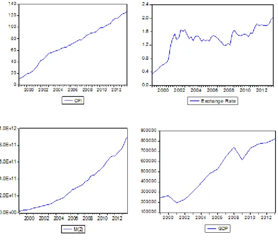
We used quarterly observations obtained from Organization for Economic Co-Operation and Development website22 which covers a period between first quarter of 1999 and last quarter of 2013. We considered four variables; consumer pricing index (CPI), exchange rates (XRE), money supply (M) and gross domestic production (GDP) which are detailed below:
XRE : End of period Exchange Rate ( Liras per Dollar, buying rates) M2: Money in billion TL
CPI: Consumer Price Index (2010=100) GDP: Real GDP (2010=100)
Figure 1: Plots of Time Series
22
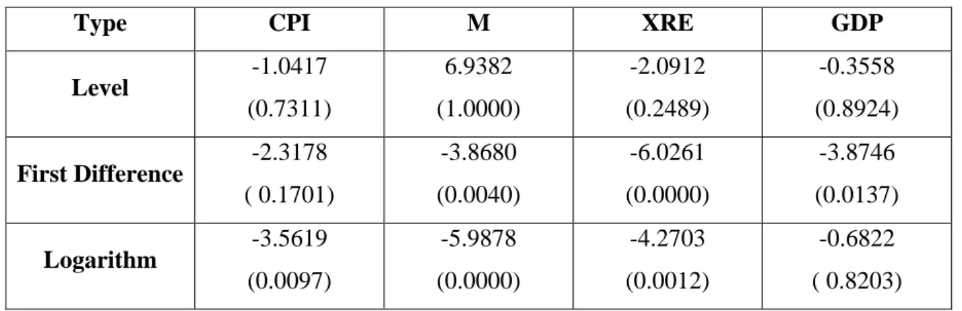
Figure-1, illustrates the data used in the study. It is clear that the processes of all variables seem to follow an increasing trend. Therefore, they are non-stationary. Table-1 contains ADF (Augmented Dicky Fuller) test results of the series along with their first differences and logarithms.
Table 1: Unit Root Test Statistics
Type CPI M XRE GDP
Level -1.0417 (0.7311) 6.9382 (1.0000) -2.0912 (0.2489) -0.3558 (0.8924) First Difference -2.3178 ( 0.1701) -3.8680 (0.0040) -6.0261 (0.0000) -3.8746 (0.0137) Logarithm -3.5619 (0.0097) -5.9878 (0.0000) -4.2703 (0.0012) -0.6822 ( 0.8203)
(Values in the parentheses show p-values.)
The results indicate that all series are I(1) except CPI which is I(2) process since we cannot reject unit root for both level and difference series for CPI. On the other hand, the log-series of the variables -which we feature in our analysis-, are all stationary except GDP.
4.3) Estimation Methodology and Results 4.3.1) Maliszewski’s Equation
Maliszewski’s Equation is an ordinary OLS model that aims to explain the behavior of inflation with macroeconomic variables rather than fitting in an ARIMA (Autoregressive Integrated Moving Average) type model. The model, however, includes an error correction variable which is especially used for dealing with non-stationary data. Nevertheless it is useful for stationary processes too. Here, we examine difference of log series which are stationary as seen in Table-2.
Table 2: Unit Root Test Results of Δ Log-Series
Dependent Variable Variable Coefficient Std. Error t-Statistic Prob.
Δ log(Pt) D(LOGCPI(-1)) -0.28361 0.088588 -3.20138 0.0023
Δ log(Et) D(LOGXRE(-1)) -0.66539 0.202707 -3.28252 0.0019
Δ log(Mt) D(LOGM(-1)) -0.64408 0.139776 -4.60796 0.0000
23
Now, by following Maliszewski’s Equation, we can write the model as
i t i t n i i i t n i i i t n i i i t n i i t P E M Y ECM P
1 1 1 1 1 0 where, 1 2 1 2 1 2 0 1 1 t t t t t P M E Y ECM As seen above, the model aims to catch short term effects of macroeconomic variables rather than its does for longer periods. This may gain advantages compared to other methods in the context of adaptivity to new information which is not conceivable for ARIMA type models.
To perform the model we first obtain the residuals of the regression between log Pt and logEt, logMt, logYt. This procedure yields the ECM (Error Correction Model). After obtaining residuals, we regress Δlog Pt on the differences of logarithms of other macro variables along with ECM. Table-3 shows the results of the fitted model.
Table 3: Regression Results for Dependent Variable: Δ log(Pt)
Variable Coefficient Std. Error t-Statistic Prob.
ΔLn(Mt-1) 0.352329 0.067963 5.184111 0 ΔLn(Pt-2) 0.343366 0.087681 3.916085 0.0003 ΔLn(Mt-2) 0.161257 0.071071 2.268956 0.0275 ΔLn(Et-2) 0.076639 0.042177 1.817075 0.0751 ECMt-1 -0.14688 0.049559 -2.963744 0.0046 C -0.010035 0.005611 -1.788438 0.0796 Adjusted R2 : 0.739885
We omitted the insignificant values except ΔLn(Et-2) which is significant at 10% level.
This is due to the fact that the model with Δlog(Et-2) has a higher Adjusted R2 than the model
without it. The results show that GDP has no effect in explaining inflation. On the other hand, second order lag of Δlog(Pt) is significant while the first lag of Δlog(Pt) is insignificant.
Furthermore, we also observe that the first and second order lags of Monetary Supply and the first order lag of ECM are significant.
24
To check if the model satisfies the OLS (Ordinary Least Squares) assumptions we applied several tests (further details are provided in Appendix C) which are summarized in Figure-4 and Table-5. These tests are performed to confirm whether our structural model may be used for a forecast study. Before proceeding with these findings we provide further explanation of our model.
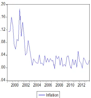
First, we observe the significant coefficient of the lagged inflation showing the impact of previous inflation values on current values. Because its coefficient is the second largest value, we can understand that inflation inertia exists in Turkey because inflationary expectations played an important role for Turkish inflation. Therefore, a percentage point increase in ΔPt-2 increases inflation by
around 0.34 percentage points.
Figure 2: Quarterly Path of Turkish Inflation
Besides, the negative coefficient of the error correcting model shows effect of the long run adjustments to Turkish inflation. So, when inflation diverge from its long run way, it adjusts to its fair value with a speed equivalent to the coefficient value of ECM. In other words, if inflation is higher than the long run rate, the model, given its negative coefficient, adjusts inflation to the expected long run value of ECM’s coefficient.
25
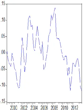
Furthermore, we need to check whether the price level is cointegrated with the macro variables considered for the theoretical model. If the residuals are I(0), we can say that the variables are cointegrated. The Figure-3 shows the path of the residuals obtained from the regression described above. Therefore, it shows that the residuals follow a stationary trend. The test statistic results below also shows that the residuals are I(0), because the probability value represent the stationary behavior of residuals. Therefore, we reject the null hypothesis of non-stationarity. Thus, we can say that price level is cointegrated with exchange rates, output, and money.
Figure 3: Plot of Errors
Once the cointegration among Ln(Pt), Ln(Et), Ln(Mt), and Ln(Yt) is established,
it remains for commenting on the long run feature between the variables. The results below show the long run impacts of Ln(Et), Ln(Mt), and Ln(Yt) on Ln(Pt). (Please look at the
appendix B for more details.)
Null Hypothesis: ECM has a unit root Exogenous: None
Lag Length: 0 (Fixed)
t-Statistic Prob.*
Augmented Dickey-Fuller test statistic -2.120374 0.0337
Test critical values: 1% level -2.604746
5% level -1.946447
26
Table 4: The Effects of Variables
Dependent Variable: Ln(Pt) Variable Coefficient Intercept -6.877173 Ln(Et) 0.539701 Ln(Mt) 0.415474 Ln(Yt) 0.558099
The results above show that the price level is positively related to the growth in money, output and exchange rate. This result is compatible with the theoretical suggestion, as the growth in output and money and a depreciation of the currency causes an increase in inflation in the long run. Therefore, one percentage point increase in exchange rate, money and output increases inflation by an amount equivalent to the value of coefficients. That is, in the long run, a one percentage point increase in exchange rate, money and output increases inflation respectively by around 0.53, 0.41 and 0.55 percentage points.
Next, we proceed to see if the model is stable enough to use for a forecast model.
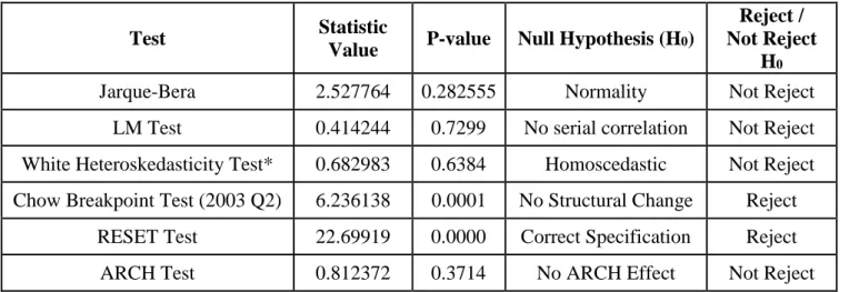
Table 5: Test Results for Reliability of Maliszewski Model
Test Statistic
Value P-value Null Hypothesis (H0)
Reject / Not Reject
H0
Jarque-Bera 2.527764 0.282555 Normality Not Reject
LM Test 0.414244 0.7299 No serial correlation Not Reject White Heteroskedasticity Test* 0.682983 0.6384 Homoscedastic Not Reject Chow Breakpoint Test (2003 Q2) 6.236138 0.0001 No Structural Change Reject
RESET Test 22.69919 0.0000 Correct Specification Reject ARCH Test 0.812372 0.3714 No ARCH Effect Not Reject
27
Figure 4: Histogram for Normality
By Jarque-Bera test statistics, we cannot reject the normality of residuals. On the other hand, we cannot reject homoscedasticity according to Breusch-Pagan-Godfrey test statistics, and from LM test results we do not see serial correlation between residuals. Besides ARCH test supports these results; thus, we cannot reject that the residuals are distributed IID N (0,1) and that there is neither serial correlation nor heteroscedasticity in the residuals. As a result, constructing the model on the basis of the normally distributed homoscedastic errors is good enough for a forecast study.
However, RESET test results are not desirable since we reject the null hypothesis that the explanatory variables are correctly specified. Yet, in grand scheme of the results the model is reliable. 0 2 4 6 8 10 -0.02 0.00 0.02 0.04 Series: Residuals Sample 1999Q4 2013Q4 Observations 57 Mean -3.41e-18 Median -0.002927 Maximum 0.052574 Minimum -0.034838 Std. Dev. 0.020156 Skewness 0.496311 Kurtosis 2.718888 Jarque-Bera 2.527764 Probability 0.282555
28
Figure-5 shows a plot of the recursive residuals about the zero line. Plus and minus two standard errors are also shown as the dotted lines at each point. Residuals outside the standard error bands show instability in the parameters of the equation. Therefore, around 2001, 2007 and 2008 parameters of the equation seem to become slightly (2008 is the heaviest) unstable due to the financial crisis. This instability is also determined with the structural break point identified with the chow breakpoint tests above.
Figure 5: Plot of Recursive Residuals
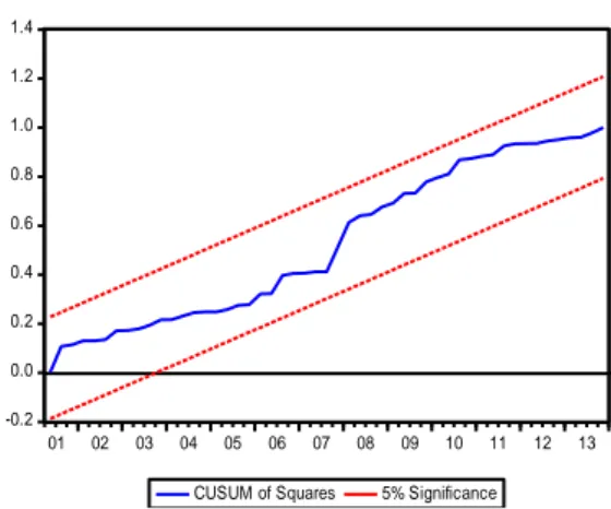
Figure-6 and Figure-7 plot the cumulative sum together with the 5% critical lines. Therefore, we try to find parameter instability if the cumulative sum tend to go outside the area between the two critical lines. According to the figures, we can say that our parameters are stable since the line stays in between the 5% critical lines. Therefore, we can obtain good forecast results using our regression model.
Figure 6: Plot of Cumulative Sum Figure 7: Plot of Cumulative Sum of Squares
-30 -20 -10 0 10 20 30 01 02 03 04 05 06 07 08 09 10 11 12 13 CUSUM 5% Significance -0.2 0.0 0.2 0.4 0.6 0.8 1.0 1.2 1.4 01 02 03 04 05 06 07 08 09 10 11 12 13 CUSUM of Squares 5% Significance
-.08 -.06 -.04 -.02 .00 .02 .04 .06 .08 01 02 03 04 05 06 07 08 09 10 11 12 13 Recursive Residuals ± 2 S.E.
29
Figure-8 is The One-Step Forecast Test, which produces a plot of the recursive residuals and standard errors and the sample points whose probability value is at or below 15 percent. From this plot we spot the least successful periods around years 2006, 2008 and 2011 since the points with p-values less the 0.05 correspond to those points where the recursive residuals go outside or approximate to the two standard error bounds. In Figure-9, N-step probability test computes all feasible cases, starting with the smallest possible sample size for estimating the forecasting equation and then adding one observation at a time. The points outside the band again show the least successful periods.
Figure 8: One-Step Probabilities Figure 9: N-Step Probabilities
Consequently, looking at the recursive coefficient below figures, we can say that all variables have significant variances in the short run. Generally, the recursive coefficient graphs of the variables in the model have sudden movements in parts but stabilize at new level. However, the variables seem to stabilize as more data over the sample period are added in the medium and the long run. The coefficients of ΔEt and ΔMt, seem to follow a more
stable path when the model uses more data. Nevertheless, the coefficients of the first lag ECM become negative given the application of the same procedure. There is only instability on intercept and it is significantly different than zero. In addition, since a lot of data is used, the coefficient of the first lag of inflation becomes positive.
Even though we observe variations in the recursive coefficients figures, they usually appear only one time and they are relatively small. Therefore, we can say that our model can be compatible to forecast inflation considering the previous tests.
.000 .025 .050 .075 .100 .125 .150 -.08 -.04 .00 .04 .08 01 02 03 04 05 06 07 08 09 10 11 12 13 One-Step Probability Recursive Residuals 0 -.08 -.04 .00 .04 .08 01 02 03 04 05 06 07 08 09 10 11 12 13 N-Step Probability Recursive Residuals
30
Figure 10: Recursive Coefficients
Table 6: Explanation of Variables
-0.2 0.0 0.2 0.4 0.6 0.8 1.0 01 02 03 04 05 06 07 08 09 10 11 12 13 Recursive C(1) Estimates ± 2 S.E. -2 -1 0 1 2 3 01 02 03 04 05 06 07 08 09 10 11 12 13 Recursive C(2) Estimates ± 2 S.E. -.4 -.2 .0 .2 .4 .6 .8 01 02 03 04 05 06 07 08 09 10 11 12 13 Recursive C(3) Estimates ± 2 S.E. -1.0 -0.5 0.0 0.5 1.0 1.5 01 02 03 04 05 06 07 08 09 10 11 12 13 Recursive C(4) Estimates ± 2 S.E. -3 -2 -1 0 1 01 02 03 04 05 06 07 08 09 10 11 12 13 Recursive C(5) Estimates ± 2 S.E. -.3 -.2 -.1 .0 .1 .2 01 02 03 04 05 06 07 08 09 10 11 12 13 Recursive C(6) Estimates ± 2 S.E. Variable Coefficient Indicator C(1) Δlog(Mt-1) C(2) Δlog(Yt-2) C(3) Δlog(Mt-2) C(4) Δlog(Et-2) C(5) ECMt-1 C(6) Coefficient
31
4.3.2) ARMA(p,q) Model
As a second model, we consider ARMA(p,q) model which is a common approach in the forecasting literature. Rather than using plain vanilla, various of its modulations are used in forecasting, however using it in its simples form gives insight for a behavior of a stationary process and helps to use it as a benchmark when comparing it with different models.
ARMA(p,q) process is a combination of autoregressive process with order of p and moving average process in order of q. Its general form is;
t q i i t i p i i t i t
c
Y
Y
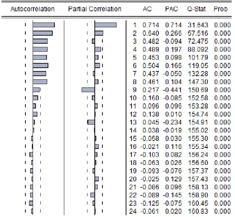
1 1Here p and q are lag orders to detect the effect of past noise or price levels on today's price. In this sense, autocorrelations (AC) and partial autocorrelations (PAC) are often referred to give insight for the lag orders. To this end we will first present the correlogram of log Pt
32
Figure-11, implies positive autocorrelation in high order with significant partial autocorrelation. This indicates that impact of early levels is long for a while and the impact of early noises is not ceasing rapidly. Hence, we apply ARMA(3,2) for p,q ϵ {1,2,3}.
4.3.3) ARMA (3,2) Model
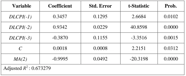
Table 7: ARMA(3,2) Results on Δ log(Pt)
Variable Coefficient Std. Error t-Statistic Prob.
DLCPI(-1) 0.3457 0.1295 2.6684 0.0102 DLCPI(-2) 0.9342 0.0229 40.8598 0.0000 DLCPI(-3) -0.3870 0.1155 -3.3516 0.0015 C 0.0018 0.0008 2.2151 0.0312 MA(2) -0.9995 0.0492 -20.3198 0.0000 Adjusted R2 : 0.673279
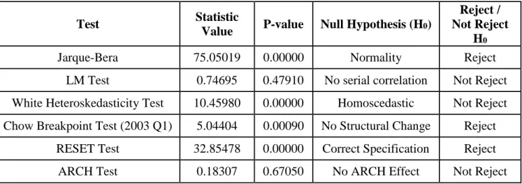
Here, we reject null hypothesis that coefficients are equal to zero at 5% significance level and model has a relatively high Adjusted R2. Results implies that in Turkish case, inflation is highly correlated with the annual realizations of second order lag of moving average process.
To check the reliability of the results we will check if the model satisfies the OLS assumptions. At first look to correlogram on residuals23, we can say that there is no AC or PAC 5% significance level. But, we need further analysis to test the reliability of the model. Findings are summarized results in Table-8.
33
Table 8: Test Results for Reliability of ARMA(3,2)
Test Statistic
Value P-value Null Hypothesis (H0)
Reject / Not Reject
H0
Jarque-Bera 75.05019 0.00000 Normality Reject
LM Test 0.74695 0.47910 No serial correlation Not Reject White Heteroskedasticity Test 10.45980 0.00000 Homoscedastic Not Reject Chow Breakpoint Test (2003 Q1) 5.04404 0.00090 No Structural Change Reject
RESET Test 32.85478 0.00000 Correct Specification Reject ARCH Test 0.18307 0.67050 No ARCH Effect Not Reject
LM test results also confirm that there is no serial autocorrelation in the residuals. Moreover, neither White Heteroskedasticity Test nor ARCH test rejects homoscedasticity, thus the model satisfies the OLS assumptions.
On the other hand, according to Chow Breakpoint Test, there is a structural break in the first quarter of 2003 which is consistent with consequences of new economic policies of the new government elected after 2002.
Lastly, normality of residuals is not supported by Jarque-Bera test. This assumption is not easily satisfied, but often supported with some other tests. However RESET test results does not support the specification either. We skip the OLS type structural break tests on residuals since they are not supported for MA processes in E-views statistics package.
34
4.3.4) AR (2) Model
In this subsection we will also check how AR model explains the inflation data. After several trials, we fit AR(2) model to difference of the log Pt series. The results are presented
in Table-9.
Table 9: AR(2) Model on Δ log(Pt)
Variable Coefficient Std. Error t-Statistic Prob.
C 0.006801 0.005315 1.279552 0.2062
DLCPI(-1) 0.461097 0.127851 3.60653 0.0007
DLCPI(-2) 0.318088 0.125217 2.540289 0.014
Adjusted R2 : 0.552679
Results are parallel with those of ARMA(3,2) except that the third lag is omitted because of its insignificance. In contrast, Table-9 shows that both the first and second order lags of inflation have positive effect on today’s inflation as in ARMA(3,2). However neither AIC, nor Adjusted R2 is greater than the former model. On the other hand, the reliability of AR(2) draws similar picture compared to ARMA(3,2). Correlogram of the residuals24 and LM test verifies that there is no serial autocorrelation in the residuals. White Heteroskedasticity Test and ARCH test also implies that the residuals are homoscedastic. Yet, RESET test is higher as well as it is below the significance level. Considering Jarque-Bera Normality Test on residuals, the model does not satisfy the normality assumption either.
Table 10: Test Results for Reliability of AR(2)
Test Statistic
Value P-value Null Hypothesis (H0)
Reject / Not Reject
H0
Jarque-Bera 52.65655 0 Normality Reject
LM Test 1.626681 0.200681 No serial correlation Not Reject White Heteroskedasticity Test 3.411676 0.014965 Homoscedastic Not Reject Chow Breakpoint Test (2003 Q2) 6.230316 0.001094 No Structural Change Reject
RESET Test 5.345687 0.007739 Correct Specification Reject ARCH Test 0.14395 0.705873 No ARCH Effect Not Reject
35
On the other hand, the plot of recursive residuals for AR(2) model of inflation shows that the parameters became unstable around 2001, 2002, and 2011 (2001 is the heaviest). In addition, the significance bands shown with dotted lines are bigger than those of the Maliszewski’s Equation. As you see them on the graph, they follow an unstable model path until 2001 and become more stable after this period.
Figure 12: Plot of Recursive Residuals
The figures below plot the cumulative sum together with the 5% critical lines. According to the Figure-13, we can say that the parameters of AR(2) model are not stable since the line stays in between the 5% critical lines. In addition, a detailed analysis with the cumulative sum of squares shows that the parameters become unstable between 2002 and 2008 since they stay fairly outside the 5% significance band. Therefore, there is a possibility that AR(2) model may not yield good forecast results.
36
The One-Step probability test results show that the most successful periods for the AR(2) model estimations are around year 2001 and 2003 since the points with p-values less than 0.05 correspond to those points where the recursive residuals go outside or approximate to the two standard error bounds. The N-step probability test, in line with the results of the recursive residuals, shows a structural break in the economy for the period between 2001 and 2003.
Figure 15: One Step Probability Plot of AR(2) Figure 16: N-Step Probability Plot of AR(2)
Eventually, according to the recursive coefficient graphs, all variables have significant variances in the short run. However, they seem to stabilize in the medium-run but since more data are added in the period, they move to a new level in the long run. Nevertheless, the variability is very high in the coefficients in the short run since there are significant structural breaks in the economy during those periods (as confirmed in the above tests).
37
Figure 17: Recursive Coeffcients Plot of AR(2)
Table 11: Description of Coefficients Variable Coefficient Indicator
C(1) C
C(2) DLCPI(-1)
38
4.3.5) TAR Model
Considering policy changes on inflation in the last 15 years, meaningful structural changes can be observed in the series; hence, a regime switching model may help better to clarify the movements of inflation. Therefore, we will apply another model, Threshold Autoregressive Model (TAR), to catch structural changes in depreciation, crisis or periods. The basic motive behind TAR model is to fit a line for the each case when the dependent variable rises above or falls below a threshold which is determined either manually or based on an information criterion such as AIC (Akaike Information Criterion). The general formula of TAR model is;
th
P
if
P
c
th
P
if
P
c
P
Log
d t t p t l p p u d t t p t l p p l tlog
)
log(
,
log
)
log(
)
(
1 1
where p is the order of model and d is the lag-order determines the threshold. Table-12 shows the statistical results of TAR model performed on Δ log Pt25
Table 12: TAR(2) Results for Δ log(Pt)
Estimate Std. Error t-Statistic Prob.
l c 0.0267 0.0038 7.0826 0 l 1 -0.3666 0.1702 -2.01542 0.0376 u c 0.035 0.0265 1.3207 0.2064 u 1 0.5327 0.2599 2.0495 0.0583
The model with minimum AIC is attained with threshold equal to 0.03851. Thus, under the statistical results we can write TAR(2) model as;