A H M E T T A H M İL C İ T H E R I S E O F M O N E Y B il k e n t 2006
THE RISE OF MONEY: AN EVOLUTIONARY ANALYSIS OF THE ORIGINS OF MONEY
A Master’s Thesis by AHMET TAHMİLCİ Department of Economics Bilkent University Ankara September 2006
THE RISE OF MONEY: AN EVOLUTIONARY ANALYSIS OF THE ORIGINS OF MONEY
The Institute of Economics and Social Sciences of
Bilkent University
by
AHMET TAHMİLCİ
In Partial Fulfilment of the Requirements for the Degree of MASTER OF ARTS in THE DEPARTMENT OF ECONOMICS BİLKENT UNIVERSITY ANKARA September 2006
I certify that I have read this thesis and have found that it is fully adequate, in scope and in quality, as a thesis for the degree of Master of Arts in Economics.
--- Asst. Prof. Kevin Hasker Supervisor
I certify that I have read this thesis and have found that it is fully adequate, in scope and in quality, as a thesis for the degree of Master of Arts in Economics.
--- Asst. Prof. Neil Arnwine Examining Committee Member
I certify that I have read this thesis and have found that it is fully adequate, in scope and in quality, as a thesis for the degree of Master of Arts in Economics.
---
Asst. Prof. Emre Alper Yildirim Examining Committee Member
Approval of the Institute of Economics and Social Sciences
--- Prof. Erdal Erel
ABSTRACT
THE RISE OF MONEY: AN EVOLUTIONARY ANALYSIS OF THE ORIGINS OF MONEY
Tahmilci, Ahmet
M.A., Department of Economics Supervisor: Assis. Prof. Kevin Hasker
September 2006
This paper shows that if there are more goods than money in all trading periods then nonconvertible fiat money is evolutionarily successful in complex economies. This result is developed in Kiyotaki and Wright (1993) search model of money, using a learning algorithm developed by Marimon et. al (1990). When we include an evolutionary model similar to Kandori, Mailath, and Rob (1993) we find that fiat money is frequently evolutionarily successful. To be precise let x be the probability someone finds someone who has a good they want –small x represents a complex economy– and let µ be the fraction of people holding money in any trading period. As long as µ < fiat money will be evolutionarily successful.
Keywords: Fiat Money, Learning, Stochastic Evolution 1-2x
1-2x 2-2x
ÖZET
PARANIN ORTAYA ÇIKIŞI: PARANIN KÖKENİNE İLİŞKİN EVRİMSEL BİR ANALİZ
Tahmilci, Ahmet Master, İktisat Bölümü
Tez Yöneticisi: Yard. Doc. Dr. Kevin Hasker
Eylül 2006
Bu çalışma, eğer ortamda sirkülasyondaki paradan fazla tüketim maddesi var ise, bu şartlar altında gelişmiş ekonomilerde geri dönüşümü olmayan kağıt paranın evrimsel olarak başarılı bir şekilde ortaya çıktığını göstermektedir. Bu sonuç Kiyotaki ve Wright (1993)’ın para araştırma teorisi modelinin Marimon et. al (1990) da kullanılan öğrenme algoritması kullanılarak değiştirilmesi ile oluşturulan model üzerinde gösterilmiştir. Bu modele Kandori, Mailath, ve Rob (1993)’ un modelindekine benzer bir evrimsel model adapte edilmesiyle kağıt paranın evrimsel olarak başarılı bir şekilde ortaya çıktığını gördük. Modeli eksiksiz bir şekilde kurmak için x istediği tüketim malzemesini ekonomideki bir başkasında bulma ihtimali – küçük x ekonominin kompleks olduğunu göstermektedir- ve µ ekonomide herhangi bir periodda parayı kullanan insan sayısı olarak kabul edelirse, kağıt para µ < koşulu sağlandığı sürece evrimsel olarak başarılı bir şekilde ortaya çıkacaktır.
ACKNOWLEDGMENTS
I would like to thank Asist. Prof. Kevin Hasker and Assist. Prof. Erdem Basci for their guidance and support during the prepeartion of this thesis. Especially, I am truly grateful to Asist. Prof. Kevin Hasker for his supervision and for being helpful in every possible ways during my two years at Bilkent University.
I would also like to thank members of my committee for their support and insightful feedback.
TABLE OF CONTENTS
ABSTRACT ... iii ÖZET ... iv ACKNOWLEDGMENTS ... v TABLE OF CONTENTS ... vi CHAPTER 1: INTRODUCTION ... 1 CHAPTER 2: MODEL... 72.1 The Model of Trading ………... 7
2.2 The Model of Learning ……... 9
2.3 The Model of Evolution ... 14
CHAPTER 3: THE STEADY STATE EQUILIBRIA ... 17
CHAPTER 4: LEARNING ………... 23
CHAPTER 5: THE EVOLUTION ………... 27
CHAPTER 6: CONCLUSION ... 32
BIBLIOGRAPHY ... 34
LIST OF FIGURES
Figure 5.1 Switching between monetary and barter equilibrium... 29
CHAPTER 1
INTRODUCTION
Why do people exchange intrinsically worthless paper money for valuable goods? How money became the basic exchange tool in the market? It has long been studied why money is Pareto superior to barter but how did economies make the transition? Money as a medium has evolved through the very essence of what it has created, a desire to specialize, to compete in its market and to advance, but it is also a consequence of the specialization of market. Namely, this is a cyclic process: specialization leads to money and money leads to specialization; and in this paper, we argue inception was initiated by specialization of the market. Kiyotaki and Wright (1993) developed an elegant analytical model that has both barter exchange and monetary exchange equilibria, but this model can not explain the transition between the
two. Money is money since society perceives it as valuable1 and if people think money is valuable then they will use money. In this paper, we are trying to answer the question how the transition occurs, and the transition dynamics from the barter equilibrium to the monetary equilibrium via a learning based game-theoretic model is the main emphasis of this paper.
To develop a model of how society switches between these two viable equilibria we need to have a model of how people behave out of equilibrium. One that has recently been subjected to analysis in the microeconomics literature is the model of stochastic evolution---first developed by Kandori, Mailath, and Rob (1993) and Young (1993). When we apply this general model to the evolution of money it implies that people occasionally try out money, and once enough people have decided to use fiat money others are slowly convinced that it is best, until in the end it is the primary mechanism of trade. We show that this transition occurs surprisingly frequently. As long as there are more real goods than fiat money produced in each trading period then in complex economies fiat money is evolutionarily dominant (or stochastically stable in the terminology of the literature.)
We have to modify the basic model of evolution because using money is an equilibrium in a dynamic game---one accepts money today so one can buy things tomorrow. Out of equilibrium the calculation of continuation values is very complicated, so we use a feedback learning algorithm developed by Marimon, McGratten, and Sargent (1990). We modify this algorithm and show that people using
the modified feedback-learning algorithm are able to learn in a wide variety of environments. With the basic algorithm Lettau and Uhlig (1999) show people may falsely learn a sub-optimal strategy to be superior to the optimal rule. In our model people always learn the optimal strategy from interaction and positive feedback and this allows us to predict which strategy will survive the evolutionary process. Thus independent of the initial beliefs, agents learn the value of money and beliefs converge to the true values of the infinite horizon optimization problem. Hence, in our model agents learn the equilibrium path from interaction and positive feedback.
However notice that our learning rule will be history dependent. Thus people should be aware that their current beliefs might sometimes be wrong, and we consider agents who sometimes try out new beliefs; this is what we called modified algorithm. This transforms the interaction into one of dynamic evolution. With these perturbations in the system agents switch back and forth between the barter and fiat money equilibrium. The switches to the evolutionarily dominant strategy will be more frequently---infinitely more frequent as the probability of trying out new beliefs goes to zero---and this allows us to make a unique long run prediction.
Further, our feedback learning model is a different approach to stochastic evolution literature, it allows us to consider just the last key assumptions of the classic evolutionary model and other two assumptions are naturally satisfied by our model. As developed by Kandori, Mailath, and Rob (1993), stochastic evolution makes three behavioral assumptions: inertia, myopia, and mutations. Inertia means that not all agents
change their strategy in every period, and in our model this happens naturally since agents' beliefs change based on the classifier-strength system which is updated every period. Myopia means that one chooses the action that is optimal given the current distribution of the population, and our learning model explicitly explains how beliefs are formed and then replaces this with just choosing the optimal action given one's beliefs. The only element of their model that we directly adopt is mutations. Mutations mean that very rarely people change their strategy at random, in our model people develop radical new guesses about the continuation values.
As noted above, people may have wrong beliefs about their current state and we allow simple experiments are necessary for learning. In our model, for example, if someone does not occasionally experiment with trading he could believe that not trading is always best. We handle this type of simple experiment by having people occasionally take the wrong actions.
If we look at the literature of search-theory of money we see that the majority of the traditional literature has been focused on explaining why money is Pareto Superior to barter. One common conclusion of this literature is that a primary benefit of money is in overcoming the famed double coincidence of wants---an insight first developed by Jevons (1875). In a barter economy by the general matching rule you must both find someone who wants what you have and has what you want, while in a monetary economy you only need to find someone who has what you want. This insight has been used in a spate of recent papers that try to explain the transition from a barter economy
to a monetary economy. Most of these papers use variations of the model developed by Kiyotaki and Wright (1993). For example in Ritter (1995) the money stock in the market is not pre-determined, rather the money issuing incentive can optimally introduce its currency and the stock in the market. However since that is an equilibrium analysis it has to assume people are willing to use money. This type of analysis can not explain how people learn to trust money. There are some other variations of the basic model such as Zhou and Green (2002) allow for a finite life time; Williamson and Wright(1994) allows for divisible money and goods; and Kehoe, Kiyotaki, and Wright (1991) allow for the possibility of private information. However, these modifications do not address the fundamental deficiency of needing people to believe that money is good before they accept it.
There is a strain of this literature that analyzes what occurs under various learning dynamics. The seminal paper on learning is Marimon, McGratten, and Sargent (1990); and others modify that model to improve on those results. For example Basci (1999) in his learning model based on Kehoe, Kiyotaki, and Wright (1991) includes learning from neighbors and shows people learn more quickly. Other papers use simpler learning algorithms and focus more on the evolutionary aspect of the analysis. Iwai (2001) uses a ``bootstrap'' argument to explain when commodity and fiat money can arise. Wright (1999) uses an evolutionary argument to show that barter and fiat money cannot co-exist as methods of exchange. Wright (1995) shows that the commodity with the lowest storage cost will naturally become commodity money. Selgin (2003) shows that even if fiat money is possible when they start out using barter, learning procedure
leads the good with the lowest storage cost to emerge as commodity money. These articles emphasize our key point. We have to look at models where agents occasionally conduct ``grand experiments.'' Only by analyzing this type of model can we hope to discover whether people will learn to trust money.
In the next section we introduce the model in three parts. First we introduce the basic interaction, then our model of learning, and then our model of evolution. The rest of the paper mimics this three step presentation. First we find the steady state equilibria of the model in chapter 3. Then we show that our learning algorithm will work, and show that this means society will learn in chapter 4. Finally we show which strategy will be stochastically stable (or evolutionarily dominant) in section 5. We then conclude.
CHAPTER 2
MODEL
2.1 The Model of Trading
Let us consider a world with I infinitely lived agents (I should be even and large) with heterogenous abilities and needs. There are n consumption goods which are indivisible. Each individual is endowed with a fixed ability to produce one of n goods and a fixed need to consume another one of n goods. Assume that each period everyone is endowed with one unit of a good that they can not consume, thus they must trade. This good is neither durable nor divisible, thus it must be either traded for a unit of consumption good or wasted. Next period each agent will be endowed with a unit of consumption good again.
must find someone who wants what they have (call this event a) and has what they want (call this event b), while if they use money they only have to find someone who has what they want (event b). Let the probability of each of these events be x (<1) then barter occurs with probability x2; money trading with probability x. Since x> x2 there is a utility of money.
We will change the endowment of some agents to one unit of fiat money (a fraction µ =i/I, i Є{ 4,6,8,...I-4}. This good is not consumable but it is durable, enabling trade across periods. It is also a substitute for barter, thus someone with a unit of money will never be endowed with a unit of consumption good. Now we have a model where agents can trade either using barter or fiat money.
Agents will be matched with each other by equal likelihood, and when two agents {i,j} are matched there are nine possible situations. Player i can have what j wants, call this cj; or i can not have what j wants, call this c-j; or i can have money, denoted m. Likewise agent j can have what i wants---ci, have a good i does not want---c -i, or be endowed with money m. This means that the nine states of the world, called as
state space, are Ω = {cj, c−j,m} × {cj, c−j,m}.
Each period, after matching occurs agents decide whether to trade (T) or not (N) based on trading partner's endowment. We denote the action set of the trading partners as Ai=Aj={ T,N} , and A= Ai
x
Aj. If both choose to trade then the exchange takes place, otherwise it does not.If person i trades for a unit of ci then he gets utility U>0, if he trades for a unit of
c-i then he incurs a transaction cost of к>0, if he trades for a unit of money he gets no utility but does not incur a transaction cost.2 Next period (which is discounted with a factor of β Є (0,1) someone with money can trade for a unit of consumption good. Notice that this means that the interaction is dynamic, the value of money today depends on what occurs next period.
We would like to specifically mention the two simplifications in this model that make it the most divorced from reality. First of all there is no central agency that issues the fiat money and controls the quantity of money. This allows us to ignore the incentives of the central agency that is issuing the fiat money and the issue of seignorage. For an article that addresses these issues one can refer to Ritter (1995). His key result is that the body issuing the fiat money has to represent a large enough fraction of the population using the money for there to be a fiat money equilibrium. There is also no price level since goods and money are not divisible.
2.2 The Model of Learning
An important problem in economics and other areas of science is finding the mathematical relationship between the empirically observed variables measuring a system. Especially, in a dynamic interaction the calculation of returns is extremely
2
If к=0 then our results are simpler without changing in any significant way. We will note the changes this would cause below. In our analysis we will make the traditional assumption that к>0.
difficult. In a steady state it is relatively simple but our model will usually not be in steady state, since we are trying to look at the out of equilibrium behavior of the economy. Out of steady state, one must estimate the path of motion of the economy, which requires estimating the other individuals' decisions, and then calculate the optimal strategy. Notice that in order to estimate other individuals' decisions one must calculate their beliefs about the path of motion of the economy.
Related to the issue of finding the equilibrium path of the economy, genetic
algorithms provide a better assistance as equilibrium selection devices in the models with multiple equilibria and the examination of transitional dynamics that accompanies the equilibrium selection process. As some applications show, these algorithms can also be used as models of individual learning where evolution takes place on a set of competing beliefs of an individual agents. If the objective of research is the examination of strategic interactions in game-theoretic framework, then individual learning is a more appropriate paradigm. Techniques similar to those used in evolutionary game theory could be used in some of the models to examine the local stability of equilibria under the evolutionary dynamics. In addition, the analysis of the asymptotic behavior of the simplified versions of models can improve our understanding of simulations and provide support for the observed behavior. These algorithms impose low requirement on the computational ability of economic agents. (Arifovic (2000))
One model developed by Marimon, McGratten, and Sargent (1990) and Lettau and Uhlig (1999) does have the features described above and could be a good starting
point for our model. In this model, people begin with guesses of what the value of various strategies is, and then use an explicit ad-hoc learning algorithm to find the true values.
While this type of model has only recently been analyzed in economics we should mention that it has a long history in other literatures. One of the ground breaking works in this field was Chris Watkins' dissertation in Psychology (1989). We should note that our model is consistent with two well-known facts from psychological learning literature, called ''Law of Effect'' and ''Power Law of Practice''. ''Law Of Effect'' says that choices that have good outcomes in the past are more likely repeated in the future, and in our model by the classifier-strength system good outcomes in the past favors the same outcome in the future by the positive feedback to the belief of the value for that outcome. Second, ''Power Law of Practice'' states that the slope of learning curve is decreasing in time, and in our model this assumption is satisfied easily by the concave learning curve.
As well Computer Scientists have longed analyzed models in this class; see Barto, Bradtke, and Singh (1995) for a review of this literature and some new results. Notice that the Psychologists are seeking a reasonable model for human behavior while the Computer Scientists are seeking the most efficient learning algorithm. Despite these divergent goals they both have analyzed the type of model we consider here.
value of an action pair α ЄA at the state ω Є Ω. We denote the strength at time t, Stαω, and the column vector of these strengths as St (for initial strength the column vector is
S0). Each period this person observes the state of the world and using St choose the action with the highest expected strength. Then he updates the strength of the state that actually occurs. Let τ Є( 0,1) be the weight they put on their old strength, and Uαω be the instantaneous payoff from the action pair α at the state ω, then:
St+1αω=(1-
τ
) Stαω+τ
(Uαω+β
M tαωSt)otherwise St+1α’ω’= Stα’ω’. The row vector Mtαω is the Markov transition probabilities in period t given { α, ω}. These transition probabilities will be a function of the
distribution of strategies from last period, this agent's strategy, and experiments (discussed below.)
There are several differences between this model and the general model in Lettau and Uhlig (1999). These differences are primarily motivated by a desire to be certain agents can learn. We argue that this is a type of ``long run rationality.'' Clearly in the short run agents will make mistakes because they have the wrong priors, however if they also are making mistakes in the long run this suggests not only are their priors wrong but their model of the interaction is wrong. Most of the changes we make to the model are motivated by this difference.
The first of the changes we make to the model is that like Basci (1999) we have one strength for each action/state pair and thus our agents choose an optimal action at each state instead of optimal strategies. Notice that optimal strategies are made up of
optimal actions at each state, thus in our model if St-1αω is correct and the distribution of strategies is not changing, agents will choose the optimal strategy. If we instead had them choosing strategies then either we rule out a-priori players using certain strategies or we have a model which is equivalent to the one here. Since ruling out strategies a-priori is anathema to unbiased analysis we favor the simpler model. Our assumption that they have a different strength depending on the action of their opponent is made for technical convenience.
The second difference is that we assume agents experiment---there is some fixed εex>0 that they choose the wrong action at every state. As Watkins (1989) shows this enables learning because every state is reached with positive probability. Without this assumption an agent could reach silly conclusions like never trading is optimal.(Note that Lettau and Uhlig (1999) calls this ''good state bias'') All results in this paper will be for small εex.
Two final changes are dictated by the environment we are analyzing. In Marimon et al.(1990) the update factor (τ) is decreasing over time. As Benveniste, Metivier, and Priouret (1987) point out this is only sensible if the optimal strategy cannot change over time. In our model there are multiple equilibria and thus the optimal strategy can change. If τ
→
0 this means that agents are ignoring new information, and thus the agents might be making worse and worse decisions as time goes by.for by another change. In the standard model Mt is just what happened to agent i in period t. This is one reason that they assume that τ
→
0, without this assumption the model may never converge. Thus we assume that Mt is based on the population distribution of strategies from last period. We are fairly certain our results would hold ifMt was based on a partial sample (similar to Young (1993)) but are certain our results fail if it is based only on personal experience.
We want to allow for very general priors on the strengths, all we require is that they are drawn from a compact and continuous support that includes all feasible payoffs, or that any S0 ∈
[
-κ/(1-β), U/(1-β)]
|A||Ω| is possible.2.3 The Model Evolution
When we add one refinement to our model of learning it will be a model of stochastic evolution. We will assume that with probability εm >0 people mutate, or draw
St-1 from the initial distribution. We can justify this as checking to make sure if your historic beliefs are correct (one should consider low
τ
) but we notice that this addition to the model completely changes results. Because of this society will not settle down at any particular state. Instead society will constantly adopt new strategies. However as εm→
0 society will spend most of their time around a particular state, some situation where everyone is best responding to the current distribution of strategies. This will mean that society is spending most of it's times near limit sets.1. Any distribution of strategies in the limit set can be reached from any other without mutations.
2. Any distribution of strategies that is not in the limit set can only be reached via mutations.
Intuitively this is a ``best response cycle.'' i.e. if the distribution of strategies is currently at one distribution in the limit set, and everyone best responds to that then the distribution of strategies is at another. Clearly any Nash equilibrium is a limit set, but there might be others. In this interaction, however, there will not be.
We will be interested in the system when is εm very small. As εm →0 the relative likelihood of any other event dwarfs the likelihood of a mutation. Thus the number of mutations needed to transition from one limit set to another will completely determine how likely the transition is. Here this will be some fraction, η, of the population, and for given I we will need mutations.3 This dependency on I will be unimportant for the analysis, and we will say that a fraction η of the population must mutate.
The only transition that will matter in this paper is the transition that takes the least mutations, this transition determines the radius.
Definition 2: The radius of a limit set π is the least fraction of the population that must
change their strategy before in the long run a player can not use a strategy in π, we
3
For a real number x, is the smallest integer which is larger than x, and is the largest integer that is smaller.
denote this r∗(π).
Intuitively the reader might find it easier to think of the radius as a ``security level.'' In this interaction if fewer than this fraction stop using a strategy in the limit set then it can be ignored. A person can be secure that they are using the right strategy without qualification.
CHAPTER 3:
THE STEADY STATE EQUILIBRIA
In this section we will ignore the model of learning and evolution for a while, and focus on the steady state equilibria of the underlying game. In order to carefully analyze learning and out of equilibrium behavior we need a simple method of representing every possible strategy. One method is to list the states at which this strategy trades. Then, for example, the always trade strategy is:
and the never trade strategy is NT={
∅
}.of the learning algorithm if εex =0. If one starts out with the beliefs that not trading is optimal then one will never have any experience that will change one's mind(Lettau and Uhlig (1999) calls this ''good state bias''). This is an example of why experimentation is important, and for all εex>0 this strategy is strictly dominated.
Lemma 1: Trading for ci is a dominant action. So is not trading at the state { cj,c-i}
and { c-j,c-i}.
Proof: See the appendix on page 37.
This pins down an optimal strategy at five of the nine states of the world. Furthermore the strategy at {m,m} does not affect payoffs so we will ignore it.4 This leaves only three states left to specify a strategy at: {cj,m}, {c-j,m}, and {m,c-i}. The important steady state equilibria each trade at a subset of these states. These are:
B is a barter strategy, if you are using this strategy and holding money you will take anything to get rid of it. F is the fiat money trading strategy, in this strategy you will trade anything in order to hold money. Notice that everyone barters if it is feasible, one always is willing to trade for ci.
If agents make mistakes too frequently, or β is too low, then trading for c-i when holding money might never be optimal. In this case instead of the B strategy everyone
will use the B~ strategy:
When we call something an ``equilibrium'' we mean it is a Nash equilibrium, but notice that since people make mistakes with strictly positive probability this is also a Subgame Perfect equilibrium and a Sequential equilibrium. Furthermore, since people base their decisions on strengths it is probability zero that they will be indifferent between actions, thus we assume people use pure strategies.5 When we call a strategy a ``pure population equilibrium'' we mean that everyone in the population is using the same pure strategy. When we call a strategy ``mixed population equilibrium'' this means that some people are using different pure strategies.
In order to characterize the equilibria we need to calculate the continuation values of holding a consumption good c or money m.
Lemma 2: (Charachterization) The continuation values from holding money and a consumption good are:
where Pg ( s) is the probability of trading for good g Є { ci,c-i,m } when holding sЄ{c,m}
5
and .
Proof: One can easily calculate that the flow values of these states are:
and after algebraic manipulation these can be turned into the continuation values above.
With this result we can quickly find the pure population equilibria.
Lemma 3: F and B are the pure population equilibria unless agents are impatient or
experiment a lot. If β< or εex >ε*ex then B~ is an equilibrium instead of
B.
Proof: See the appendix on page 38.
Note that as we mention above if people experiment a lot or people discount feature beliefs too much, trading for c-i is never optimal. As a result, B~ is an equilibrium in stead of B.
In the rest of the paper we will assume that B is the pure population barter equilibrium without loss of generality, indeed our proofs would be easier if trading at {
m, c-i } were never a best response.
none of them do agents use the strategy B. The reason for this is that B trades at the state
{m, c-i} because the value of holding money is so low that the cost of к is worth the benefit of holding a consumption good. In a mixed population equilibrium the value of holding money is higher, and thus it is not a good idea to trade money for c-i. There is a continuum of mixed population equilibria because in such an equilibrium agents are indifferent between using the strategy F and F~:
but the value of holding money is decreasing the more people use the strategy F, and thus for each mixture we have a different equilibrium.
Notice that agents might also use strategies other than B~,F and F~ in a mixed population equilibrium. We might, for example, have some people who only trade for money when holding c-j. Thus the entire space of equilibria is complicated, and not worth specifying. The only important equilibria in our analysis are the extremes, where all agents who trade for money are using either the strategies F or F~. Let πm (f) be the fraction of the people holding money who use strategy f Є{ F, F~} and πc (f) be the equivalent portion holding the consumption good.
Lemma 4: The extreme mixed population equilibria are
Proof: See the appendix on page 39.
Notice two interesting facts about these equilibria. First, as Wright (1999) show the mixed population equilibrium requires more people to be using money than a mixed strategy equilibrium. In a mixed strategy equilibrium anyone will trade for money thus πm (f)
≈
πc (f), while in a mixed population equilibria essentially everyone who is holding money will be using a fiat money strategy. Secondly notice these equilibria are not stable, if in any period less than πc (f) fiat money traders are in the consumption state a barter strategy is a strict best response. Finally notice that the equilibrium condition depends only on πc (f). In fact (as we will have to assume later) they could have incorrect beliefs about πm (f) and as long as πc (f) is at it’s critical value this will be sufficient.66
This is the final point where к=0 has a real impact on our analysis. \ One can check that if к=0 then
CHAPTER 4
LEARNING
In this section we will specify the steady states of our learning algorithm. The first proposition merely establishes that we have met our criteria of ``long run rationality'': agents can learn. If this result did not hold then we would argue that we had misspecified the learning algorithm. The second proposition is not a result we assumed a priori, this proposition shows that the population can learn simultaneously. The results of the first proposition we are certain work in very general environments since our learning algorithm is similar to a Gauss-Seidel learning algorithm, the results of the second proposition may not hold in all games.
One key decision we have to make at this point is what information people will have about the current distribution of strategies and how they should interpret this
information. One option is to have them know the distribution of strategies dependent on whether people are holding money or not. This would be the most information we could assume they have, and we argue it is too much. While explicitly they will know the distribution in each period implicitly we wish the distribution to represent some general information they have gathered. This information might be old and not completely trustworthy. Thus they should not be able to deduce exactly how many people are using a certain strategy today, and whether those people are holding a consumption good or money. Furthermore is it reasonable to assume they know the distribution over strategies? A strategy is not directly observable, it requires many observations of a person to know his entire strategy. Thus we will only let them know the fraction of people who trade in each state, η={ ηω}ωЄΩ.
This assumption, however, presents us with some secondary issues. These issues will not strongly affect analysis but must be addressed. Given the distribution of actions what are agents' beliefs about the distribution of strategies? The simplest assumption would be that the two distributions are independent, but these beliefs would be wrong any time society is not in equilibrium, or the beliefs fail a ``reasonability'' test. We notice that our learning algorithm induces a correlation between actions, and we assume that agents understand this correlation. This leads us to four simple conclusions. First if an agent is taking one dominant action then they are taking all dominant actions. If they are not taking all of their dominant actions and they trade for ci when holding cj (or c-j) then they also trade when holding c-j (or cj). If they trade at { m, c-i } then they do not
trade at {cj ,m} or {c-j ,m}. Finally if they trade at {cj ,m} then they trade at {c-j ,m}. Of course all these assumptions are made only to the extent they are possible given η.
These are all fairly transparent, the final issue we must address is the strategies of agents who are holding money. We have two options, either we could have them calculate πm (f) or we could simply have them assume that with probability one someone who is holding money is using a fiat money strategy. The former assumption requires them to be able to do complicated calculations, and furthermore would not be that different from the latter when εex is small. Thus we will assume that the fraction who hold money will first be made up of people who trade at {cj ,m} and then any excess will be made up of those who will trade at {c-j ,m} but not {cj ,m}. Because we assume that those who trade for money at either state will trade at both this means that the
probability someone will trade for m when i is holding cj and c-j is
P( T| cj,m)=max {η cj,m - µ, 0} and P( T| c-j,m) =max { η c-j,m -µ,0} respectively.
With these decisions made we can now focus on our learning algorithm. The convergence of our learning algorithm is immediate since εex>0. With this assumption our problem is equivalent to the Gauss-Seidel method of value calculation. Thus convergence is guaranteed.
Proposition 1: If only one person learns then he will learn all of his strict best responses.
By this result, we guarantee individual learning , but as we said above there is no guarantee that one person being able to learn implies that society is able to learn. Hence, we need a result that leads us to social learning.
Kushner (2005) has worked on games where the population has two agents and proved that the Gauss-Seidel algorithm converges to a steady state, but it is unclear if these results apply to our environment. Thus here we address the simpler problem of showing that in this game the population learns.
Proposition 2: There is an I such that if I ≥ I_ society almost surely converges to an
equilibrium.
Proof: See the appendix on page 41.
By this proposition we show that if we have enough people to trade with and agent can learn their strict best responses, population can learn its best response. Notice that this proposition would be simpler if agents knew the current distribution of strategies. In that case we could have all of one group trade for money, and at the current distribution either a fiat or barter strategy would be a best response.
CHAPTER 5
EVOLUTION
We now will show when evolution will result in a society using fiat money. The first step of our analysis is to find the radii of our equilibria. Notice that in our model we do not only need to know what strategies people are using but what their strengths are. However as εm→ 0 if a society is in a limit set they will be there for a long time, thus their strengths will be nearly equal to the true values.
Lemma 5:
∀
I∃
εex > 0 such that if εex ≤ ε˜ex then r∗
(F)=(1− πc (F))(1 − µ) andr
∗
(B)=(1− µ) πc(F˜)+ µ, and if π∗
is a mixed population equilibrium r∗
(π∗
) =limξ→01/I.As one can see if the population size is large, mixed population equilibrium is hard to observe in the society, unless each agent in the population is convinced to use it. Otherwise, if there is more than one agent who is willing to use some other equilibrium, society will be out of equilibrium, and result in either monetary equilibrium or in barter equilibrium.
Note that this is one of the key results of this paper. We stated security levels for the barter, monetary and mixed equilibria. In other words, we specify critical mass of agents to change the equilibrium from one to another. For example, a fraction of population which is less than r
∗
(F), does not effect the state of the world. However, if there is a fraction grater than r∗
(F) is willing to use barter trading, then new equilibrium for the whole population becomes barter equilibrium. As a result, the system does not rest in any state and it switches between these equilibria stated in the lemma. We can note that this is due to the ergodicity of our model, i.e. each agent may try out of equilibrium path by learning and by mutations.Further, our learning based evolutionary algorithm give place for switching between equilibria. We show that society may switch barter equilibrium whenever there is enough fraction who wants to switch from monetary equilibrium or it may switch to monetary equilibrium while using barter equilibrium given that there is enough fraction who is willing to use money.
Also, one can see that if we are interested in the rise of fiat money then we have made the worst assumption about how agents estimate the fraction of people holding money and using the fiat money strategy. We have assumed that they always over estimate the fraction using the fiat money strategy, if we required them to calculate the correct probability or believe that strategy and the good being held were independent this would make the transition from barter to fiat money easier. Secondly, notice that
r
∗
(F) and r∗
(B) are determined by the fraction of agents holding money and by the fraction of the population who uses fiat money strategy while holding the consumption good, namely πc(f),f Є{ F, F~}.Thirdly, from lemma 3 limεex→0 πc*(F)
≈
πc*( F~)≈
x. Using simple algebra, one can easily find r∗
(F) > r∗
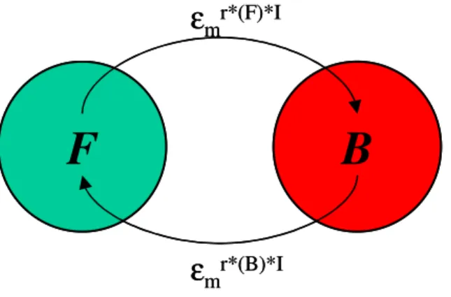
(B) , and by the definition of the security level in the long run monetary equilibrium is more stable than barter equilibrium, since the least fraction of the population that must switch their strategy from monetary equilibrium is greater than the fraction for the barter equilibrium. In other words, in our model if society learns to use money, then we expect that society will use monetary trading most of the time, since to switch from monetary equilibrium we need more agents than to switch from barter equilibrium.F
B
ε
mr*(F)*Iε
mr*(B)*IF
B
ε
mr*(F)*Iε
mr*(B)*IFigure 5.1 Switching between monetary and barter equilibrium
Before we state our final result, we should note that these results reveal the consistency of our model with the history since even in complex economies there is a place for barter trading and historically agents sometimes utilize barter even they use money as a medium of exchange.
Now, the final result can be explained very succinctly. The most interesting case is when εex is nearly zero and the society is complex---x is nearly zero---or it is hard to find someone who wants to trade with you. In this case the only important parameter is µ, and if µ<1/2 then fiat money will be evolutionarily dominant or stochastically stable.
Theorem 1: If I ≥ I and εex ≤ε--ex and there is less money than goods (µ < 1/2) then in
complex societies non-convertible fiat money is stochastically stable when εex is nearly
zero. More generally this is true when:
where Proof: See the appendix on page 45.
Notice that agents using the fiat money strategy do barter if the opportunity arises. We should point out that this occurs even today, while the majority of trades use money people do not turn down the opportunity to barter. In our model agents rarely use barter in complex societies. The general formula for the probability that a trade uses money in the fiat money equilibrium is
2µ/[2µ+ x2 (1
−
µ)] (3)One simple model of x is that it is the inverse of the number of goods an agent consumes, thus in a modern economy x=1/1000 would be conservative. If this is so and µ ≥1/20 then more than 99% of trades will use fiat money.
CHAPTER 6
CONCLUSION
It has long been wondered how non-convertible fiat money came to be trusted. We all recognize the optimality of money, this has been explained in many frameworks and many different models. The question is how people came to trust a worthless piece of paper, enough that they would give up real goods for these wooden nickels. We show that in complex economies as long as the market is not flooded with this worthless currency people will learn to trust it.
In fact the most surprising fact, given our analysis, is that non-convertible fiat money has taken so long to arise. As Dowd (2001) points out fiat money has never arisen in a barter economy historically. It has always been preceded by commodity money---with gold being the primary example, then by fractionally based commodity
money, and then pure fiat money has only arisen through government fiat---hence the name.
Thus while our results show that fiat money can arise they do not show how fiat money did arise historically. To understand this issue we first need a tractable and reasonable model where all four different strategies could be equilibria. Right now there is no paper that includes all four equilibria in a tractable model. Iwai (2001) analyzes a model with all of the relevant equilibria, but the equilibria depend on the distribution of agents' types and thus would not be suitable for analysis. Selgin (2003) has a tractable model with fiat money, commodity money, and barter as possible strategies but that model does not have a barter equilibrium.
There are several issues that would need to be addressed in the final version of such a model. One issue that Dowd (2001) raises and our model does not address is how do people choose between currencies? We believe that it is uncommon in history that multiple currencies are accepted---early United States history being a counter example. Why is this? One part of this analysis should include exchange rates, and for that we would need to have divisible goods and currency as in Green and Zhou (2002). Another line of analysis is looking at the incentives of the party issuing the currency. In our model the stock of currency is a given, but in Ritter (1995) this depends on the incentives of the issuing body. Our results here would require that this body represents a significant fraction of the population. We hope that the our basic results add to the understanding of this issue, and that with further analysis we can develop a complete understanding of the rise of money.
BIBLIOGRAPHY
Arifovic, J. (2000) Evolutionary Algorithms in Macroeconomic Models.
Macroeconomic Dynamics 4: 373-414.
Barto, A., Bradtke, S., Singh, S. (1995) ``Learning to act using real-time dynamic programming.'' Artificial Intelligence . 72.
Basci, Erdem. (1999) ``Learning by Imitation''; Journal of Economic Dynamics and
Control, 23:1569-85.
Benveniste, Albert; Michel Metivier; and Pierre Priouret. (1987). Adaptive Algorithms
and Stochastic Approximations. Springer-Verlag; Berlin.
Dowd, K. (2001) ''The Emergence of Fiat Money: A Reconsideration'' Cato Journal. 20: 467-76.
Ellison, Glenn. (1993): ``Learning, Local Interaction and Coordination.'' Econometrica, 61:1047-1071.
Ellison, Glenn. (2000): ``Basins of Attraction, Long Run Equilibria, and the Speed of Step-by-Step Evolution.'' Review of Economic Studies, 67:1-23.
Hasker, Kevin. (2004) ``The Emergent Seed: Simplifying the Analysis of Dynamic Evolution.'' Bilkent Economics Department Discussion Paper 04-06. Available at: http://www.bilkent.edu.tr/\symbol{126}hasker/Research/Hasker-Emergent-Seed-05-08-26.pdf.
Iwai, Katsuhito. (2001). ``Evolution of Money.'' in The Evolution of Economic
Diversity. Antonio Nicita and Ugo Pagano, eds. Routledge, London and New York.
Jevons, W. Stanley. (1875). Money and the Medium of Exchange. King, London.
Kandori, Michihiro; George Mailath, and Rafael Rob. (1993): ``Learning Mutation, and Long Run Equilibria in Games.'' Econometrica, 61:9-56
Kiyotaki, Nobuhiro and Randall Wright. (1993). ``A Search-Theoretic Approach to Monetary Economics. American Economic Review. 83:63-77.
Kushner, Harold J. (1972) Introduction to Stochastic Control Theory. Holt, Reinhart, and Winston; New York.
Kushner, Harold J. (2005) ``Numerical Approximations for Non-Zero-Sum Stochastic
Differential Games.'' mimeo, available at:
http://www.dam.brown.edu/lcds/papers/Num-Games-non-zero.pdf
Lettau, Martin and Harald Uhlig. (1999). ``Rules of Thumb versus Dynamic Programming.''American Economic Review. 89:148-174.
Marimon, R.; E. McGratten; T.J. Sargent. (1990). ``Money as a Medium of Exchange in an Economy with Artificially Intelligent Agents.'' Journal of Economic Dynamics
and Control. 14:329-373.
Ritter, Joseph. (1995). ``The Transition from Barter to Fiat Money.''American Economic Review. 85:134-149
Selgin, George. (2003).``Adaptive Learning and the Transition to Fiat Money''.
Economic Journal, 113:147-65.
Watkins, C. (1989). ``Learning with Delayed Rewards.'' Ph.D. thesis, Cambridge University, Psychology Department.
Wright, Randal. (1995) ``Search, Evolution, and Money.'' Journal of Economic
Dynamics and Control, 19:181-206.``
Wright, Randall. (1999) “A Note on Asymmetric and Mixed Strategy Equilibria in the Search-Theoretic Model of Fiat Money.'' Economic Theory, 14:463-471.
Young 1993}}Young, Peyton. (1993): ``The Evolution of Conventions.''
APPENDIX:
Proof of Lemma 1.
If i trades at {c−j, c−i} and j trades with probability ηj . > 0 the trade will take place with probability (1 − εex) ηj. . If i does not trade then the trade will take place with probability εexηj . < (1 − εex) ηj . . Thus trading is not optimal since it gives an instantaneous loss of κ and in the next period has the same continuation value as not trading. The same argument also explains not trading at {cj, c−i} and inverting the argument explains trading at {cj, ci} and {c−j, ci}.
Now consider not trading at {m, ci}. To clarify the following argument given a strategy σ let the value of holding a unit of money between periods be V (m|σ), and V
(c|σ) be the value of holding a unit of a consumption good. Assume that i meets someone with a unit of ci, then if i trades they get U + βV (c|σ) if they do not trade then they get 0+βV (m|σ). The proof will be done when we establish upper bounds for V
If the strategy calls for trading at {m, c-i} then by optimality we know that −κ + βV (c|σ) ≥ 0+βV (m|σ) and we are done. Thus the strategy must require no trading at {m,
c-i} and {m, ci}.
If εex = 0 then V (m|σ) = 0 < U + βV (c|σ) since V (c|σ) ≥ 0 by optimality. Thus if there is a εex such that 0 + βV (m|σ) > U + βV (c|σ). V (m|σ) must be increasing in εex. But
V(m|σ) =(1− (1 − µ) εex) (0+βV (m|σ)) + (1 − µ) εex (xU − (1 − x) κ + βV (c|σ)) (4) ∂V (m|σ)/∂ εex = (1− µ) ((xU − (1 − x) κ + βV (c|σ)) − (0 + βV (m|σ)))
and ∂V (m|σ)/∂ εex≤ 0 when xU − (1 − x) κ + βV (c|σ) ≤ 0 + βV (m|σ), thus the highest
0 + βV(m|σ) can be is xU − (1 − x) κ + βV (c|σ) which is strictly less than U + βV (c|σ). Therefore for all εex, U + βV (c|σ) > 0 + βV (m|σ).
Proof of Lemma 3.
In order for the F strategy to be a best response we need that:
V (m|F) ≥ V (c|F) (5)
or
(P ci (m) − P ci (c))U ≥ (P c−i (m) − Pc−i (c))κ (6) and this requires that:
(1 − µ) (1 − εex) x (1 − x) (1 − 2 εex)U ≥ −(1 − µ) (1 − x) x εex (1 − 2 εex) κ (7) since the right hand side is negative this will be true as long as εex < 1/2. In order for B˜ to be a best response we need that:
(Pci (c) − Pci (m))U ≥ (Pc−i (c) − Pc−i (m))κ (8)
(1 − µ) (1 − εex) x2 (1 − 2 εex)U ≥ (1 − µ) (1 − x) x εex (1 − 2 εex) κ
and this requires that εex < min{1/2, xU/(xU+(1−x)κ)} in order for B to be a best response we also need that:
βV (m) ≤ −κ + βV (c) (9)
or
(Pc−i (c) +(1 − β)/β+ Pci (m) + Pm (c))κ ≤ (Pci (c) − Pci (m))U (10)
If εex = 0 and β > κ/[(1−µ)x2U+κ] one can easily show this is true. One can also show that the left hand side is increasing in εex and the right hand side is decreasing and that when εex = 1/2 the right hand side is zero and the left hand side positive. Thus there is a maximal εex for each β such that this holds, and this is the ε*ex in the statement of the lemma.
Proof of Lemma 4.
In a mixed population equilibrium one can show that:
Pci (m)U − Pc−i (m) κ = Pci (c)U − Pc−i (c) κ (Mixed Pop. Condition) After solving for the probabilities and substitution this gives us:
πc (f) = x + (1 − x) κεex{[(α (f) − εex) πm (f)]/(1 − 2 εex)-x}/ (1 − εex) xU (11)
where α(F) = (1− εex), α(F˜) = εex. Note that from this equation we can see that πc(F) = πc(F˜) + [εex(1−x)κ πm (F)]/[(1− εex)xU], and that πc(F˜) is independent of
πm(F˜), thus we know that πc (F) < πc (F˜). The equation equalizing the inflow and outflow of players in the money state is:
πm(f)(1 −πc(f))(x (1−εex) εex+(1− x)ε2ex)= πc(f)(1−πm(f))[x(1 − εex)2+(1 − x)εexα (f)] (12)
(oio (εex |f) πm(f))/(1 − πm(f)) = πc(f)/(1 − πc(f)) and after manipulation these are equivalent to the conditions in Lemma 4.
Proof of Proposition 1.
The proof is done when we rewrite our algorithm so that it is transparently a Gauss-Seidel learning algorithm. To do this choose any arbitrary sequence over Ω and any arbitrary sequence over A for each Ω, being sure that the last action pair is {T,T}, since εex> 0 this sequence has strictly positive probability. Then note that since others are not changing their strategy Mt = M (σi) where σi is this player’s strategy. Then we can rewrite our formula for St+1αω as:
Stαω = (1
−
τ ) St-1αω + τ [Uαω + β Mαω (σi) St-1] (13)Stαω = τ Uαω + Dαω (σi) St-1 where
D(σi) = (1
−
τ ) I|A|∗|Ω| + τ βM (σi) (14) (IZ is an identity matrix with Z rows) and our agent chooses ai (ω) asai (ω)
∈
arg maxαi∈{T,N}Eαj [Stαiαjωi] (15)Skω= maxαi∈{T,N} Eαj [τUαiαjω+ D(σi (αi)) St−1] (16)
where where σi(αi) reflects the dependence of σi on the player choosing αi at state ω. As Kushner (2005) shows since ΣjDij = (1 − τ)+τ β < 1 the vector {Skω}ω∈Ω converges to the optimal value function, thus our {Stαω}αω ∈A×Ω converges
to the true values of the optimal strategies. (Note that the strategy will converge in finite time. Once the strategy converges we can ignore the σi in equation (13) then we can be sure that the {Stαω}αω ∈A×Ω converge to their true value.)
Convergence to the optimal strategy will happen in finite time on this sequence. Let ζ > 0 be the least difference in continuation values for actions that have a strict best response. Then since the strengths converge to the true values there is a finite T such that the difference between all optimal values and the current strengths are strictly less than 1/2 ζ and will be forever after. At this point the player will be using the optimal strategy.
Since T is finite this subsequence is finite and in each period a player has a strictly positive probability of entering it. Thus a player learns almost surely.
Proof of Proposition 2.
Choose I large enough so that if a player’s best response is not independent of what four other are doing then there are at least four people who are trading at {cj,m} and four people who are not.
Notice that in order to implement Proposition 1 we need to have a group of two people who are holding money and two people who are holding a consumption good. For this Proposition we also need them to be using the right strategies.
If the best response of any player is independent of what four people are doing then we can choose the group at random, being sure that as many as possible are not best responding at the state {cj,m}. Otherwise we need the four people in the group to all not be best responding at the state {cj,m}.
To achieve a group of this sort implement a finite sequence of trades so that there are two groups–one of whom is trading at {cj,m} and one of whom is not. If this is not possible in a finite number of trades then everyone must be either trading or not at
{cj,m} and we are done, thus assume that it is possible. Therefore without loss of generality select the group that is not best responding at {cj,m}.
Have the people in the group go into a finite subsequence as specified in
Proposition 1, at the end of this subsequence all players in the group will have learned to best respond at all states. While this group is in this subsequence have everyone not
in this group be in matches that either reinforce dominant actions or involve trading money.
At this point everyone’s best response will be independent of what four people do, thus we can form a random group of four with as many non-best responders as possible and repeat this process. By iteration we can be sure everyone will best respond, and then we can have everyone learn one final time so that their value functions will coincide with the fact that everyone is now using a best response.
Proof of Lemma 5.
We first note that if we are in a mixed population equilibrium we can have one person switch to either F or B˜ and then we can use Proposition 2 to converge to either the F or B equilibrium.
First notice that if all players are using the B strategy that for all λ > 0 and κ > 0 there is a εm > 0 such that if the probability of a mutation is less than this εm, P([St −
V(B)] < κ) > 1− λ for all people in the society. This is an immediate implication of
Proposition 1 and the fact that mutations only occur with probability εm. Thus we can assume all people are using the strategy B and that [St − V (B)] < κ, where the value of κ will depend on the population size and be selected below.
Then clearly if people mutate to the F˜ strategy
than people mutate. We will show that behavior will return to all people using B.
Clearly the most difficult case will be when mutants do not learn their true values, so have them either trade using dominant actions or trade money. Furthermore it will be insufficient if someone using the B strategy switches to the B˜ strategy, so what we must show is that there is no sequence where someone using the strategy B˜ will switch to F˜.
Now assume that − 1 people mutate to the F˜
strategy. Then we know that since I is discrete V(c|B˜)− V(m|F˜)≥ 2κ > 0 for all εex. Let this be the κ we used above. Notice as well that in this case the value of every strength will increase since when some people are using the F˜ strategy this increases the value of money. This means that for all {αω} Stαω − S*αω is negative, thus every time {αω} is updated Stαω − S*αω will be negative, or all strengths will approach their new limit from below.
What we must show is that trading at the states {cj,m} and {c-j,m} is not optimal for someone who is using the B strategy. Now for someone using the B strategy the initial value of the strengths {St{N,T}{cj,m}, St{N,N}{cj,m}, St{T,N}{cj,m}} are all at least
[(1−εex)(1−µ)βx2U]/(1−β)+εexβZ1(εex)−κ where Z1(εex) is a function such that
limεex→0Z1(εex)=0. As well given the new distribution of strategies V(c|B˜)=
[(1−εex)(1−µ)x2U]/(1−β)+εexZ2(εex) where limεex→0Z2(εex)= Z2> 0. Since
V(c|F˜)≤V(c|B˜)−2κ≤ [(1−εex)(1−µ)x2U]/(1−β)+εexZ2(εex)− κ and the limiting value of St{N,T}{cj,m} is β V(m|F˜) there clearly is a ε˜ex such that
[(1−ε˜ex)(1−µ)βx2U]/(1−β)+ε˜exβZ2(ε˜ex)− βκ <[(1−ε˜ex)(1−µ)βx2U]/(1−β)+ε˜exβZ1(ε˜ex) (17) ε˜ex (Z2(ε˜ex) − Z1(ε˜ex)) < κ
and if this is true then even if St{N,T}{cj,m} is at it’s initial value and St{T,T}{cj,m} increases to it’s limiting value it will still be true that St{T,T}{cj,m}< St{N,T}{cj,m}.
Thus all people will choose either the strategy B or B˜ even if the learning process favors the strategy F˜. This argument is clearly reversible because the only difference between B˜ and F˜ is whether you trade at the state {cjm}. Note that if people are using F instead of F˜ this only has an impact on order of εex, thus for small enough εex the statement is correct.
Proof of Theorem 1.
From Young (1993) we know that a limit set (equilibrium in this game) is stochastically stable if it has the minimum stochastic potential. From Hasker (2004) we know that the
stochastic potential of an equilibrium σ
∗
is:c
∗
σ∗ = c∗
(E) − r∗
(σ∗
) + ca(σ∗
) (18) where E is the emergent seed and ca (·) is the core attraction rate. Notice that in order to find the stochastically stable strategy we do not actually need to find the emergent seed (which we will not), and we will show that for the relevant equilibria ca (σ∗
) ≤ 1/I .First we will dispatch with the possibility that a mixed population equilibrium could be stochastically stable. Assume to the contrary that π
∗
has the lowest stochastic potential, notice that we can transition from the π∗
equilibrium to F with only one mutation, this means that:c
∗
F≤ c∗
π∗ +1/I − r∗
(F) (19)and clearly this is negative for reasonable I.
Now the core attraction rate is the number of mutations to get from the core to the given strategy. The core must contain more than one limit set thus it either contains both F and B or it contains a mixed strategy equilibrium. This tells us that the maximum of the core attraction rate is 1/I as claimed above.
Given this F must be stochastically stable if:
which will be true for large enough I if (1