Exchange rate determination: effect of Turkish and global macroeconomic news

(1)

ii

EXCHANGE RATE DETERMINATION:

EFFECT OF TURKISH AND GLOBAL MACROECONOMIC NEWS

THE GRADUATE SCHOOL OF SOCIAL SCIENCES OF

TOBB UNIVERSITY OF ECONOMICS AND TECHNOLOGY

MUHAMMED MÜCAHİT DENK

THE DEPARTMENT OF ECONOMICS

THE DEGREE OF MASTER OF SCIENCE

(2)

(3)

(4)

1

ABSTRACT

EXCHANGE RATE DETERMINATION: EFFECT OF TURKISH AND GLOBAL MACROECONOMIC NEWS

DENK, Muhammed Mücahit M.Sc., Economics

Supervisor: Asst. Prof. Ünay TAMGAÇ TEZCAN

This study investigates the effect of the domestic and foreign sourced macro-economic news on the increase of the TL - Dolar exchange rate observed after 2013. The study was carried out, using OLS and GARCH methods for the period between January 1, 2013 and December 31, 2016. The results reveal that surprises related to domestic macro-economic data is more effective than foreign macro-economic surprises and the most important variables that explain the movements in the exchange rate are domestic inflation and monetary policy surprises as well as foreign employment surprises.

(5)

2

ÖZ

DÖVİZ KURU BELİRLENMESİ: TÜRKİYE VE KÜRESEL MAKROEKONOMİK HABERLERİN ETKİSİ

DENK, Muhammed Mücahit Yüksek Lisans, İktisat

Tez Danışmanı: Yrd. Doç. Ünay TAMGAÇ TEZCAN

Bu çalışma 2013 yılından sonra görülen TL- dolar döviz kurundaki yükselişin sebebini yerli ve yabancı kaynaklı makroekonomik duyuruların etkilerini ele alarak araştırmaktadır. Çalışma 01 Ocak 2013 ile 31 Aralık 2016 tarihleri için OLS ve GARCH yöntemi kullanılarak incelenmiştir. Sonuçlar, yerel makroekonomik verilere ilişkin sürprizlerin yabancı makroekonomik sürprizlerden daha etkili olduğunu ve döviz kurunun hareketlerini açıklayan en önemli değişkenlerin yerel enflasyon ve merkez bankası politikası sürprizleriyle yabancı istihdam sürprizleri olduğunu göstermektedir.

(6)

3

DEDICATION

(7)

4

ACKNOWLEDGMENTS

I would like to extend a special thank you to Prof. Ünay TAMGAÇ TEZCAN, my thesis advisor, who oversaw my study. It is a valuable opportunity for me to share her time during this process. I also would like to extend my special appreciation for the academic knowledge I gained throughout this my thesis study.

A very special thank you goes to my teachers, Prof. M. Eray YÜCEL, Prof. Fatih ÖZATAY, Prof. Hüseyin MERDAN and Prof. Bedri Kamil Onur TAŞ who never gave up their support both throughout my undergraduate and graduate education, guided me with their deep knowledge and experience, and approached me with a brother’s affection rather than a scholar’s brochure.

I would like to extend a special thank you to Prof. Haldun EVRENK for teaching how a “real scientist” is through his knowledge, personality and intellectual background all throughout my graduate education.

I am deeply grateful to my dear family for always making me feel their support and prayers throughout my life and for being with me in my hard times.

(8)

5

LIST OF TABLES

Table 4. 1. Summary statistics of values of the index values ... 42

Table 4. 2. Aggregation by News Category ... 45

Table 4. 3. Aggregation by expected volatility level... 46

Table 5. 1. Summary statistics of the TL/$ exchange rate ... 47

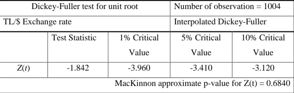
Table 5. 2. Dickey-Fuller test result of the TL/$ exchange rate ... 48

Table 5. 3. Dickey-Fuller test result of first difference of the TL/$ exchange rate ... 48

Table 5. 4. OLS result of all news ... 50

Table 5. 5. OLS results of positive news ... 51

Table 5. 6. OLS results of negative news ... 52

Table 5. 7. GARCH result of all news index ... 54

Table 5. 8. GARCH result of positive news index ... 55

Table 5. 9. GARCH result of negative news index ... 56

Table 5. 10. OLS result of country news ... 58

Table 5. 11. OLS result of country news (symmetric) ... 59

Table 5. 12. GARCH result of Turkey news index ... 60

Table 5. 13. GARCH result of US news index... 61

Table 5. 14. OLS result of news index by expected volatility level ... 62

Table 5. 15. GARCH result of news index by expected volatility level ... 64

Table 5. 16. OLS result of Category news index ... 66

Table 5. 17. GARCH result of Category news index ... 66

(11)

8

LIST OF GRAPHS

Graph 1.1. Movement of the TL/$ Exchange rate ... 13

Graph 1.2. Movement of the TL/$ exchange rate (2002-2016) ... 14

Graph 4.1. Movement of the first difference of the $/TL exchange rate ... 38

Graph 4.2. Histogram of news indexes which are not equal to zero ... 42

(12)

9

LIST OF FIGURES

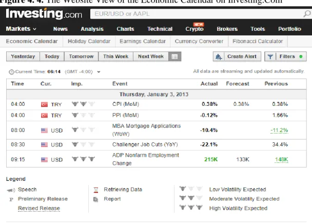
Figure 4. 1. The Website View of the Economic Calendar on Investing.com ... 39

(13)

10

ABBREVIATION LIST

API : American Petroleum Institute AR : Autoregressive

ARCH : Autoregressive Conditional Heteroskedasticity ARCH-LM : ARCH- Lagrange multiplier

ARIMA : Autoregressive Integrated Moving Average ARMA : Autoregressive Moving Average

CB : Conference Board

CBRT : Central Bank of the Republic of Turkey CPI : Consumer Price Index

DEM : Germany Deutsche Mark

DF-GLS : Dickey-Fuller Generalized Least Squares

EGARCH : Exponential Generalized Autoregressive Conditional Heteroscedastic EIA : Energy Information Administration

EMH : Efficient Market Hypothesis

EMU : Economic and Monetary Union of the European Union FED : Board of Governors of the Federal Reserve System FX : Foreign exchange

GARCH : Generalized Autoregressive Conditional Heteroskedasticity GDP : Gross Domestic Product

GFC : Global Financial Crisis

IBD/TIPP : The Investor's Business Daily/ Technometrica Institute of Policy and Politics

ISM : The Institute of Supply Management JPY : Japanese Yen

KC FED : Federal Reserve Bank of Kansas City KPSS test : Kwiatkowski–Phillips–Schmidt–Shin test

MA : Moving Average

MoM : Month-over-Month N.S.A. : Non-Seasonal Adjust

NAPM : The National Association of Purchasing Managers NFIB : National Federation of Independent Business'

(14)

11

NY : New York

OLS : Ordinary Least Squares

PCE : Personal Consumption Expenditure PMI : Purchasing Managers Index

PPI : Producer Price Index QoQ : Quarter-over-Quarter ROM : Reserve Option Mechanism S&P : Standard & Poor's

S&P/CS HPI : The Standard & Poor's Case–Shiller Home Price Indices S.A. : Seasonal Adjust

SSR : Sum of Squared Residuals

SWARCH : Switching Autoregressive Conditional Heteroskedasticity TANKAN : Tanki Keizai Kansoku Chousa

TIC : Treasury International Capital TRY : Turkish Lira

TSI : Turkish Statistical Institute US : United States

USA : United States of America USD : United States Dollar

VAR-GARCH: Value at Risk-Generalized Autoregressive Conditional Heteroskedasticity

(15)

12

CHAPTER I

INTRODUCTION

In this study, the effect of news related to macro-economic indicators on the $/TL exchange rate in Turkey is analyzed. The relationship between exchange rates and macro-economic indicators has been widely discussed in the academic literature. Studies conclude that it is difficult to estimate exchange rates using various macro indicators. While many empirical studies that analyzed the relationship between exchange rate and macro indicators have succeeded relatively on explicating long-term movements of exchange rates, they fail to explain the short and mid-term movements. In the academic literature, various approaches have been proposed towards the understanding of the dynamics related to the short and mid-term movement of exchange rates. As Ehrmann and Fratzscher (2005) cited in their studies, news surprises is an important source of information that affect markets and hence market prices. The news surprises are obtained by a comparison of the values of the actual data at the time when the data is released and the market expectations before the release time. Recently, empirical studies using this approach showed that news about various macro indicators have significant impact on the foreign exchange markets.

One important study of this nature is Neely and Dey’s (2010) study which studies the effect of news on the USA exchange rates. While there are several research on the relationship between news and exchange rate movements, studies on developing countries are especially rare. This is basically due to the lack of data and that expectation surveys are not regular for macro indicators in developing countries.

In this study, the above mentioned approach that considers the effect of news surprises on foreign exchange markets is adopted for Turkey. Specifically surprises of

(16)

13

real-time macro data obtained through news announcements for Turkey are used to explain the $/TL exchange rate. In Turkey, there are various studies that study the impact of news about monetary policy on financial markets, such as Aktaş et al. (2009), Demiralp and Yılmaz (2010), and Duran et al. (2012). However, these studies focus on the news related to monetary policy, and there is not a comprehensive study that analyses the effect of general macroeconomic news on the exchange rate. Moreover, I also incorporate macroeconomic news announcements from the US into our analysis of the TL/$ exchange rate. Hence, I jointly compare the effect of domestic and foreign news on the exchange rate.

Graph 1.1. Movement of the TL/$ Exchange rate

The investigation of exchange rate and news surprises is based on Efficient Market Hypothesis (EMH). The first traditional definition of EMH was done by Eugene Fama in 1975.1_{Thanks to this idea, Fama won Nobel Prize in 2013 along with} Lars Peter Hansen and Robert J. Shiller.2 According to EMH, prices in the market are

1_{Fama, E. F. (2011). My life in finance. Annu. Rev. Financ. Econ., 3(1), 1-15.} 2_{For more information:} http://www.nobelprize.org/nobel_prizes/economic-sciences/laureates/2013/fama-facts.html

(17)

14

influenced by all relevant news and expectations. Based on this information, prices are determined according to the laws of supply and demand.

Fama defines efficient market as the market in which all rational investors compete to maximize their interest and knowledge is accessible to all. These assumptions are also valid for the forex market where the exchange rates are determined. In this case, a new information can change the price,

In this study I will examine the impact of the news to explain $/TL exchange rate. I analyze the period between the years 2013 and 2016. This period is quite important for $/TL exchange rate because the exchange rate has experienced large fluctuations and the TL has depreciated after a long period of stability since the 2002 crises. As it can be seen in Graph 1.2, the TL/$ exchange rate which had been fairly stable between the years 2002- 2012, ranging between 1-2 for more than a decade, it has been on a gradual increase since year 2013. While the $/TL exchange rate had reached a maximum level of 1.91 in the 2002-2013 period, it has increased to 3.54 in the 3-year period from 2013 till 2016.

(18)

15

This study analyses the effects of major macro-economic news so as to find out the determinants for the increase in $/TL exchange rate since 2013. Daily data is used in the time series analysis and the estimations are carried using two different methods, namely OLS and GARCH. After an exploration of the recent literature on exchange rate determination in Chapter II, the methodology used in the study is discussed in Chapter III. Information about the data is provided in Chapter IV and the empirical finding are discussed in Chapter V. Finally, the conclusion is provided in Chapter VI.

(19)

16

CHAPTER II

LITERATURE

Recently, a considerably amount of interest is built on the understanding of how news related to macroeconomic data affect exchange rates. As discussed in Andersen et al. (2003) (ABDV (2003) hereafter) macro-economic news influence both the conditional mean returns and volatilities of exchange rates.

As the efficient market hypothesis explains, all the available information in the market must already be included in the asset prices (EMH, see Fama, 1970). Thus, asset prices must only change by the arrival of new unexpected information. These “surprises” affect the asset prices as they change agents’ expectations about the future state of the economy. Basically, they can affect the expectations related to cash flows or the discount factor. Therefore, an unanticipated change in exchange rate today can only be explained by the unexpected information connected with the arrival of new data (“news”) between the time agents’ expectations are built and the present time.

There are two basic methods in the empirical literature to model “news” to analyze how news affect the exchange rate. In the first method time series innovations in the relevant macroeconomic variables are considered as “news”. In the second one, the difference between the actual and expected values of macroeconomic announcements based on survey data is taken as “news”. Recently there is a rapidly growing empirical literature that uses news to explain exchange rate behavior. Below the most relevant studies to this study are discussed.

2. 1. Eddelbüttel and McCurdy (1996)

One of the initial studies in this literature is by Eddelbüttel and McCurdy (1996) who analyze the impact of the frequency of general and currency-specific news

(20)

17

headlines on the DEM-USD exchange rate changes. They are using deseasonalized intraday DEM-USD exchange rate changes that starts from October 1992 and ends on September 1993. They use data, named as the ‘HFDF93’ data, gathered from Olsen & Associates which includes every bid and ask exchange rates between the Japanese Yen, the German Mark, and the US Dollar. The data also includes Reuters news data set together with the relevant interest rate or yield differential. They use a GARCH (1,1) model to estimate the impacts of news headlines on the intraday volatility of the DEM-USD spot exchange rate.

One important finding of this paper is that interest rates do not have much descriptor power at a high frequency; but, that in the conditional variance equation the frequency of news and also the interest rate differential is highly significant. Particularly, more global news increases the conditional volatility of the DEM-USD spot exchange rate.

2. 2. Andersen, Bollerslev, Diebold and Vega (2003)

This paper queried whether exchange rate has a connection with news about fundamentals of the economy or not. Their study is focused on the connection among forex movements, news and order flow. They show that news effects are important for the exchange rate behavior and that there are asymmetric response patterns. They confirm that the main system is increasing the impact of bad news in good times and that – increased state uncertainty – operates in the data. Moreover, they also investigate how the stock, bond and foreign exchange markets react to real-time news surprises.

First, they have a focus on foreign exchange markets rather than a sole focus on stock or bond markets. They refer to the central issue in the exchange rate economy and the link between exchange rates and fundamentals.

(21)

18

Moreover, they primarily concentrate on exchange rate conditional means rather than conditional variances. They do not try to find out exchange rate volatility but the rate of the exchange rate itself, since without modeling the conditional mean sufficiently high-frequency discrete-time volatility cannot be extracted.

Thirdly, they use a renewed date set spanning a relatively longer time period. In addition, it involves a broad set of exchange rates and macroeconomic indicators.

2. 3. Galati and Ho (2003)

This paper investigates the impact of macroeconomic news on the daily movements of the euro/dollar exchange rate in the Euro Area and the United States during the first two years of EMU. Their daily data covers the period of January 1, 1999 to December 31, 2000.

They also query if the agents reacted to news differently or not depending on the following cases: whether it was European or a U.S. centered news, whether the news was bad or good. Also, they search if the traders’ response changes as time passes.

Their finding is that the daily change of the euro/dollar ratio is highly correlated with macroeconomic news. Nevertheless, a notable time variation is displayed in this relationship. They also show that the market reacts to bad news coming from the Euro area and that good news do not play a major role.

2. 4. Cai, Joo, Zhang (2009)

This paper investigates how macroeconomic news in the domestic economy and in the US affects exchange rates for nine developing markets. In order to achieve this, it uses a unique high-frequency data for nine emerging countries, namely Czech

(22)

19

Republic, Hungary, Indonesia, Korea, Mexico, Poland, South Africa, Thailand, and Turkey. Data from Bloomberg on market expectations on macroeconomic news and the actual announcement, and data from Consensus Forecasts on market expectations for the exchange rates is used. Using data from January 2, 2000 to the end at December 31, 2006 GARCH (1,1) model is employed in the study.

The study shows that the returns and volatilities of developing market exchange rates is highly responsive to major US macroeconomic news. In contrast, domestic news does not have much effect; and recently, the US news has become more effective on developing market currencies. The study also shows that these currencies can regularly be more reactive to market sentiment. Good news become more notable when optimism prevails in the market, and bad news become more notable while pessimism prevails. Hence, they show that macroeconomic news is statistically significant at a varying degree with market uncertainty, and the significance differs by news and currency.

2. 5. Özlü and Ünalmış (2012)

This paper considers the effect of economic fundamentals on exchange rates in Turkey. The paper uses GARCH (1, 1) model with the daily data obtained from Reuters, the Turkish Central Bank and Turkish Statistics Institute for the period from March 2004 until July 18, 2012.

In this study, the effects of announcements related to several macroeconomic variables namely the GDP, industrial production index, inflation, current account deficit, balance of trade and monetary policy on the TL/$ exchange rate is investigated using real time data for Turkey. Examination of how the exchange rates react after the announcements are made is important for the policy makers. The reaction of the

(23)

20

exchange rate to macroeconomic indicators basically reflects changes in expectations about current and future macro indicators. Their findings show that the value of the Turkish Lira is particularly sensitive to the surprises about the current account deficit and monetary policy.

2. 6. Birz and Lott (2013)

This paper considers newspaper coverage of real sector macro news and analyzes how it affects the stock returns on the S&P 500. News coverage of four macroeconomic series, namely GDP, durable goods, retail sales and unemployment, collected from the Money Market Survey is used in the study. The empirical analysis is based on daily data over the period from January, 1991 to April, 2004 and returns on the S&P 500 data are gathered from Wharton Research Data Services.

They try to find out if there is a link between stock returns and real sector economic news. The literature published before has pointed out that statistical releases determine the price of stocks by affecting agents’ expectations and decisions. And by anecdotal evidence it is said that these two are correlated however this argument lacks strong empirical evidence. Thus, as a new approach, they use newspaper coverage as representative for agents’ interpretation after macro news.

The paper shows that stock returns are highly affected by news about unemployment and GDP growth. The connection between retail sales and durable goods news and stock prices is seem to be weak, though they end up with the expected sign. Their explanation is that the variables are not directly an indicator for upcoming economic circumstances, or durable goods and retail sales may not have enough statistical strength because of insufficient report stories.

The paper points to a possible causation problem because newspaper articles are written after stock market’s closing on the day of the economic releases. To avoid

(24)

21

this problem, as another measure of economic news they use Associated Press stories, which are written earlier than stock market closure.

This paper claims that the results can be helpful to understand how real economic news affects stock market. However, since the articles are generally transmitted after economic releases it does not seem possible to make trading strategies using news articles’ information.

2. 7. Ermişoğlu, Oduncu and Akçelik (2013)

This paper analyzes how the Reserve Options Mechanism (ROM) affects the basket exchange rate calculated as an average of the dollar and euro in a period of volatile short term capital flows and in terms of macroeconomic and financial stability.

Following the global financial crisis, academics and policy makers have started to discuss a central banking framework that can contribute to financial stability as well as price stability. The ROM, which is one of such innovative policy instruments recently put into practice by the Central Bank of the Republic of Turkey. It is mainly used to reduce the adverse effects of extreme volatility in capital movements for macroeconomic and financial stability.

The paper by Ermişoğlu et al. (2013) empirically analyzes the effect of ROM on exchange rate volatility using a VAR-GARCH (1, 1) model with the daily data. The analysis period starts from October 15, 2010 which is the time the Central bank stopped to pay interest rate for the required reserves, and ends at October 15, 2012.

The paper shows that the ROM has a significant effect in decreasing exchange rate volatility during the study period. Hence their finding is that ROM is an effective policy tool for reducing exchange rate volatility caused by volatility in capital flows.

(25)

22 2. 8. Caporale, Spagnolo and Spagnol (2016)

This paper examines how exchange rates are affected by macroeconomic news coverages. In order to examine the interaction between exchange rates and macroeconomic news, this paper uses a VAR-GARCH (1, 1) model. For this model, they compare several developing country currencies and the US dollar. These developing countries are Turkey, Czech Republic, South Africa, Hungary, Korea, Indonesia, Mexico, Poland and Thailand. The equations are estimated with daily data over the sample period from January 2, 2000 to December 31, 2006. The data for the News Indices are obtained from Bloomberg. They use news coverage of four macroeconomic series, which are GDP, durable goods, retail sales and unemployment as in Birz and Lott (2013) and the number of story headlines is counted as news coverage.

This paper estimates the following equation

𝑥𝑡 = 𝛼 + 𝛽𝑥𝑡−1+ 𝛿𝑓𝑡−1+ 𝑢𝑡 (1) where 𝑥_𝑡 is the vector of variables contains exchange rate, domestic news index and USA (Eurozone) news index. 𝑥_𝑡−1 is the corresponding vector of lagged variables. 𝑓_𝑡−1 is similarly a vector and contains interest rate differential, and domestic stock. For interest rate differential the 90-day Treasury bill rate differential (vis-a-vis the US) is used. Domestic stock returns are used as proxies for monetary policy and domestic financial shocks.

This paper makes five notable contributions to the existing literature. First, it takes daily newspaper coverage of macro news (newspaper headlines) into account as a form of news that drive investors’ decisions. Second, a useful econometric framework is adopted in explaining both mean and volatility spillovers. Thirdly, they use vast amount of developing markets data. Fourth, they search the potential impact

(26)

23

of the recent global financial crises. Finally, they check for external financial shocks and domestic monetary policy shocks.

Findings of this paper show that there is a weak dynamic connection between the first moments and that only for some cases, foreign news has a negative and domestic news has a positive impact. Likewise, the 2008 financial crisis, in most cases, does not seem to be effective on mean spillovers. On the contrary, they find evidence for causality invariance, and that the volatility spillover parameters have changed due to the recent financial crisis. They also find evidence on the connection between the second moments. In many cases, they observed a sizeable downward shift has been observed. At last, they find a limited role of the two proxies (for monetary policy and domestic financial shocks) in the model. As a result, they confirm that macro news has key importance in driving FX markets for developing economies.

2. 9. Akar and Çiçek (2016)

This paper investigates the effect of new policy instruments which are the interest rate corridor, required reserve ratio and reserve option mechanism (ROM) on the volatilities of US dollar, euro, British pound and basket rate for the Turkish economy. Their empirical analysis is based on daily data over the sample period from January 2, 2002 to December 9, 2014. They use ARMA-GARCH, ARMAEGARCH and SWARCH models in their analysis.

This study shows that there is asymmetric volatility impact and that negative shocks lead to smaller exchange rate volatility than positive ones. The main reason behind this asymmetry might be the circumspection motive of economic agents. Since the amount of capital flows have increased in Turkey in the recent decade, the costs of

(27)

24

Turkish Lira credits have been more expensive than the costs of foreign loans. Private sector chooses to invest in foreign exchange to prevent insolvency situation, when a positive shock hits the exchange rate. When the economy has less volatility, economic agents may choose to buy alternative assets like stocks or treasury bonds which can procure higher returns. But when the exchange rate is affected by a positive shock, these investors may immediately change their assets with foreign exchange, so that they can put a limit to their losses arising from the depreciation.

They also provide some evidence that the ROM could decrease the volatilities of exchange rates, especially of US dollar and basket rate. However, they could not reach enough evidence in favor of the other two instruments.

2. 10. Cheung, Fatum and Yamamoto (2017)

In a recent study Cheung, Fatum and Yamamoto (2017) investigate whether the effect of macro news on the exchange rate is state- and time-dependent. In order to achieve this, they analyze how the JPY/USD rate is affected by Japanese and US macroeconomic news. Their empirical analysis is based on daily data over the sample period from January 1, 1999 to August 31, 2016. They carry out their analysis for 3 sub-periods around the Global Financial Crisis (GFC): pre-GFC, the GFC and post-GFC periods. They use OLS estimation with heteroscedasticity and autocorrelation consistent (HAC) standard errors using daily data.

They study news coverage of 23 American and 17 Japanese macroeconomic data series. US news variables are consumer spending, personal income, industrial production, consumer credit, capacity utilization, retail sales, GDP second estimate, GDP third estimate, GDP advanced estimate, non-farm payrolls, durable goods orders, business inventories, new home sales, personal spending, factory orders, NAPM index,

(28)

25

index of leading indicators, consumer price index, producer price index, consumer confidence index, housing starts, target federal funds rate and trade balance. Japanese news variables are industrial production, department and super sales value, GDP final, GDP preliminary, capacity utilization, construction orders, current account, machinery orders, overall spending, trade balance, producer price index, consumer confidence index, consumer price index, retail trade, leading economic index, TANKAN non-manufacturing index and TANKAN large non-manufacturing index.

The news surprise for news q at time t, 𝑆_𝑞,𝑡 𝑖s calculated as (𝐴_𝑞,𝑡− 𝐸_𝑞,𝑡 )/𝜎̂_𝑞,𝑡 where 𝐴𝑞,𝑡 shows the actual value of a given macroeconomic fundamental q, at announced time t, 𝐸_𝑞,𝑡 shows the expectation value of a given macroeconomic fundamental q, at announced time t and 𝜎̂_𝑞,𝑡 shows the sample standard deviation of all surprise values (𝐴_𝑞,𝑡 − 𝐸_𝑞,𝑡) with fundamental q.

Three equations to analyze exchange rates and macroeconomic news. The first equation is used:

𝑅𝑡= 𝛽0+ ∑ 𝛽𝑗𝑅𝑡−𝑗+ ∑Q𝑞=1∑𝐾𝑘=0𝛶𝑞,𝑘 𝑆𝑞,𝑡−𝑘+ 𝜖𝑡

j

i=1 (2)

where 𝑅𝑡 is the five-minute exchange rate return and 𝑆𝑞, 𝑡−𝑘 is the standardized shock of the qth macro news. J determines the lag order of exchange rate returns and Q determines macroeconomic news.

The second equation is:

𝑅_𝑡= 𝛽₀+ ∑ 𝛽_𝑗𝑅_𝑡−𝑗+ ∑ ∑ 𝛶+ 𝑞,𝑘 𝐾 𝑘=0 𝑆+𝑞,𝑡−𝑘+ ∑𝑄𝑞=1∑𝑘=0𝐾 𝛶−𝑞,𝑘 𝑆−𝑞,𝑡−𝑘+ 𝜖𝑡 𝑄 𝑞=1 𝑗 𝑖=1 (3) where 𝑆−𝑞,𝑡−𝑘= I(𝑆𝑞,𝑡−𝑘 < 0)𝑆𝑞,𝑡−𝑘 (4) 𝑆+_{𝑞,𝑡−𝑘} = I(𝑆_{𝑞,𝑡−𝑘} ≥ 0)𝑆_{𝑞,𝑡−𝑘} (5) Defining 𝐼 (∙) as an indicator function that captures the surprising news’ sign.

(29)

26

Finally, the paper estimates the following equation to measure news-by-news effect as in Andersen et al. (2003).

𝑅_𝑡 = 𝛼_𝑞+ 𝛽_𝑞𝑆_𝑞𝑡+ 𝜖_𝑡 (6) More than half of the US news are found to be influential across the whole sample. Moreover, US news is found influential for all periods: before, during, and after the GFC periods. Also, it is reported that the influence of US news is remarkably larger than that of Japanese news. They show that, although the number and composition of influential US news has almost been stable over the three mentioned sub-periods, the average effect of the significant US news has notably increased in the latter periods. The average effect of the significant US news has doubled in the post-GFC period compared to the pre-post-GFC period. Their results support the view that the effect of the effective US macro news on the exchange rate is remarkably time-dependent. Specifically, US news have become more important recently after the crisis.

Their results about Japanese news differ than that about US news and most surprisingly Japanese news seem to be losing its impact rapidly after the GFC and has become non-influential.

(30)

27

CHAPTER III

METHODOLOGY

In this section I will discuss some estimation methodologies used to analyze time series variables such as daily exchange rate. To provide a better understanding of the serial correlation that exits within a time series variable in the following sections I will first discuss the three types of models, the Autoregressive (AR) model of order p, the Moving Average (MA) model of order q and the mixed Autoregressive Moving Average (ARMA) model of order p, q.

A common characteristic of financial time series is the existence of volatility clustering which occurs when the volatility of the variable changes over time. This behavior is technically named conditional heteroskedasticity. AR, MA and ARMA models do not regard volatility clustering, because they are not conditionally heteroskedastic. So, a more sophisticated model is needed for our predictions. Autoregressive Integrated Moving Average (ARIMA), Autoregressive Conditional Heteroskedastic (ARCH) and Generalized Autoregressive Conditional Heteroskedastic (GARCH) are some examples of advanced models.

In the financial time series analysis of this study GARCH models will be used for predicting exchange rate changes. Even tough AR, MA and ARMA are more basic time series models, they can be considered as the basis for more advanced models. Therefore, more sophisticated models will be discussed after a basic introduction on the more basic models.

3. 1. Salient Financial Time Series Models

Before introducing the time series models, it will be useful to go over the concept of stationarity and the technique of differencing.

(31)

28 3. 1. a. Stationary and Differencing

A time series is called stationary if its properties (such as the mean and variance) are independent of the time in which series are observed. Time series having trend or seasonality are not stationary, inasmuch as trend and seasonality will affect the values of the series in respect to the time change.

It should be noted that a time series with cyclic behavior (but not trend or seasonality) can be stationary, because length of the cycles is not constant, so where the peaks and troughs cannot be known before observing the series.

Briefly, the patterns of a stationary time series are unpredictable in the long-term. Time plots will show the series to be roughly horizontal (although some cyclic behavior is possible) with constant variance.

The differenced series of a time series variable xt, consists of the change between consecutive observations of the original series and is stated as:

𝑥′𝑡= 𝑥𝑡− 𝑥𝑡−1 (7) Sometimes the differenced data might not be stationary and it may be necessary to difference the data once again to have a stationary series:

𝑥′′_𝑡 = 𝑥′_𝑡− 𝑥′_𝑡−1 (8) 𝑥′′𝑡 = 𝑥𝑡− 𝑥𝑡−1− (𝑥𝑡−1− 𝑥𝑡−2) (9) 𝑥′′𝑡 = 𝑥𝑡− 2𝑥𝑡−1+ 𝑥𝑡−1− 𝑥𝑡−2 (10) 3. 1. b. Random Walk

On important basic model in time series analysis is the random walk which is a time series model in which consecutive observations are equal with a random step up or down. A random walk is a time series model 𝑥_𝑡 where

(32)

29

in which 𝑒_𝑡 is the error term. The error term is a white noise, which is a normal variable whose mean is zero and variance is one.

It has to be noted that from a process of this type that the change (𝑥_𝑡− 𝑥_𝑡−1) for next period cannot be predicted. Namely, the change is absolutely random. Notice that a random walk process has a constant mean, but its variance is not constant. Consequently, a random walk process is nonstationary, and its variance increases with time t.

3. 1. c. Autoregressive Models

In multiple regression models a linear combination of predictors are used to forecast the variable of interest. In autoregression models, a linear combination of past values of the variable is used to forecast the variable of interest. Hence the term autoregression denotes that it is a regression of the variable against itself.

An autoregressive model of order p is represented as:

𝑥_𝑡 = 𝑐 + 𝜙₁𝑥_𝑡−1+ 𝜙₂𝑥_𝑡−2+ ⋯ + 𝜙_𝑝𝑥_𝑡−𝑝+ 𝑒_𝑡 (12) where 𝑒𝑡 is white noise, and c is the constant term. This equation is quite similar to a multiple regression except the lagged values of 𝑥𝑡 are the predictors. This model is referred to as the “AR (p) model”. Autoregressive models are fairly flexible in handling a wide range of different time series patterns.

For an AR (1) model:

if ϕ₁ = 0, 𝑥_𝑡 is equivalent to white noise.

if ϕ₁ = 0 𝑎𝑛𝑑 𝑐 = 0, 𝑥_𝑡 is equivalent to a random walk.

if ϕ1 = 0 𝑎𝑛𝑑 𝑐 ≠ 0, 𝑥𝑡 is equivalent to a random walk with drift.

if ϕ₁ < 0, 𝑥_𝑡 has the tendency of to swaying between positive and negative values.

(33)

30

Normally, autoregressive models are restricted to stationary data, and then it is necessary to put some constraints on the values of the parameters.

For an AR (1) model: −1 < ϕ₁ < 1

For an AR (2) model: −1 < ϕ₂ < 1, ϕ₁+ ϕ₂ < 1, ϕ₂− ϕ₁ < 1 If p ≥ 3, the restrictions become more complex.

3. 1. d. Moving Average Models

Moving average does not use past values of the forecast variable in a regression, instead it uses the past forecast errors in a regression-like model. A moving average model of order p is represented as:

𝑥𝑡 = 𝑐 + 𝑒𝑡+ 𝜇1𝑒𝑡−1+ 𝜇2𝑒𝑡−2+ ⋯ + 𝜇𝑞𝑒𝑡−𝑞 (13) Where 𝑒_𝑡 indicates white noise. This model is referred to as the MA (q) model. Since the values of 𝑒_𝑡 are not observed, it is not really a regression in the usual sense. It is important that all values of 𝑥_𝑡 can be considered as weighted moving average of the past few forecast errors. Nevertheless, moving average smoothing and moving average models should not be confused. Moving average smoothing is used in order to figure the trend-cycle of past values, on the other hand moving average models are used to forecast future values.

It should be noted that any stationary AR (p) model can be written as an MA (∞) model. If some constrains are applied on the MA parameters, the reverse –that an MA (q) model can be written as a stationary AR (∞) model–also hold. Then the MA is called “invertible” which means that any invertible MA (q) process can be represented as an AR (∞) process.

Invertible models are not simply to enable us to convert from MA models to AR models. There are some mathematical properties that make them easier in practical usage.

(34)

31

The stationarity constrains and invertibility constrains are alike. For an MA (1) model:−1 < μ₁ < 1

For an MA (2) model:−1 < 𝜇₂ < 1, 1 < 𝜇₁ + 𝜇₂, 𝜇₁− 𝜇₂ < 1 If q≥3, more elaborate conditions will hold.

3. 1. e. ARMA Models

The ARMA (p, q) model can be considered as a combination of both moving average models and autoregressive models. An ARMA (p, q) model can be represented as:

𝑥_𝑡 = 𝑐 + 𝜙₁𝑥_𝑡−1+ 𝜙₂𝑥_𝑡−2+ ⋯ + 𝜙_𝑝𝑥_𝑡−𝑝 + 𝑒_𝑡+ 𝜇₁𝑒_𝑡−1+ 𝜇₂𝑒_𝑡−2+ ⋯ + 𝜇_𝑞𝑒_𝑡−𝑞(14) In brief;

𝑥_𝑡 = c + ∑𝑝_𝑖=1ϕ_𝑖𝑥_𝑡−i+ 𝑒_𝑡+ ∑𝑞_𝑖=1μ_𝑖𝑥_𝑡−i (15) There should not be any common factors between the AR and MA polynomials; otherwise the order (p, q) of the model can be reduced.

3. 1. f. ARIMA Models

A non-seasonal ARIMA model can be formed by fusing differencing with autoregression and a moving average model. ARIMA is a word composed of the first letters Autoregressive Integrated Moving Average model (“integration” indicates the opposite of differencing). The full ARIMA (p, d, q) model can be represented as:

𝑥_𝑡(𝑑) = 𝑐 + 𝜙1𝑥𝑡−1 (𝑑) + 𝜙2𝑥𝑡−2 (𝑑) + ⋯ + 𝜙𝑝𝑥𝑡−𝑝 (𝑑) + 𝑒𝑡+ 𝜇1𝑒𝑡−1+ 𝜇2𝑒𝑡−2… + +μ_qe_t−q (16) where 𝑥_𝑡(𝑑) represents the differenced series (which may have been differenced more than once). Note that there are lagged values of 𝑥_𝑡 and lagged errors in the “predictors” on the right-hand side. In this model,

p = order of the autoregressive part; d = degree of first differencing involved;

(35)

32 q = order of the moving average part.

Some of the model mentioned before are special cases of ARIMA such that: White noise : ARIMA (0,0,0)

Random walk : ARIMA (0,1,0) with no constant Random walk with drift : ARIMA (0,1,0) with a constant Autoregression : ARIMA (p,0,0)

Moving average : ARIMA (0,0,q) 3. 2. ARCH Models

In 1982 Engle presented a basic ARCH model, the first tool allowing the variance to evolve over time. ARCH models do not take heteroskedasticity as a problem to be solved, but as a feature to be modeled. ARCH model has proved to be very good in catching the volatility clustering effect, where large (small) price changes tend to be followed by other large (small) price changes, yet of unpredictable sign. This feature is called the ARCH effect. Bollerslev (1987) explained why volatility tends to cumulate in clusters. The reason is that the intelligence reaches to economic agents in clusters, therefore volatility clustering is observed when that information is incorporated into prices.

The ARCH (q) model can be represented as:

𝑀𝑒𝑎𝑛 𝑒𝑞𝑢𝑎𝑡𝑖𝑜𝑛: 𝑦𝑡 = 𝑥𝑡𝑏 + 𝑒𝑡 (17) 𝑣𝑎𝑟𝑖𝑎𝑛𝑐𝑒 𝑒𝑞𝑢𝑎𝑡𝑖𝑜𝑛: ℎ_𝑡 = 𝑎₀+ ∑𝑞_𝑖=1𝑎_𝑖𝑒_𝑡−𝑞2 (18) 𝑒𝑡 = 𝑣𝑡√ℎ𝑡; 𝑣𝑡~𝑁(0,1) (19) where 𝑒_𝑡−𝑞2 is the past squared errors and 𝑣𝑡 is the standarlized residual. There are two equations in the ARCH (q) one for the mean and other for the variance. The equation for mean is similar to classical OLS equation having the vector of coefficients b and the error term ε𝑡, dependent variable 𝑦𝑡, the vector of independent

(36)

33

variables 𝑥_𝑡. The variance equation stands for the variance which is symbolized by ℎ_𝑡 with intercept 𝑎0 and q lags of past squared errors. These squared errors are called ARCH terms. The 𝑣_𝑡 residuals are calibrated for estimated volatility and that is why they are called standardized residuals.

3. 3. GARCH Models

The GARCH model, introduced by Bollersev, is an important extension of the ARCH model. The GARCH is acronym form of Generalized Autoregressive Conditional Heteroskedasticity model. In addition to getting along with much more flexible lag structure, the GARCH model allows for a longer memory process, which is the main advantage. The GARCH (p, q) model is represented as:

𝑀𝑒𝑎𝑛 𝑒𝑞𝑢𝑎𝑡𝑖𝑜𝑛: 𝑦_𝑡 = 𝑥_𝑡𝑏 + 𝑒_𝑡 (17) 𝑣𝑎𝑟𝑖𝑎𝑛𝑐𝑒 𝑒𝑞𝑢𝑎𝑡𝑖𝑜𝑛: ℎ_𝑡 = 𝑎₀+ ∑𝑞 𝑎_𝑖𝑒_𝑡−𝑞2

𝑖=1 + ∑𝑝𝑗=1𝛽𝑗ℎ𝑡−𝑝 (20) 𝑒_𝑡 = 𝑣_𝑡√ℎ𝑡; 𝑣𝑡~𝑁(0,1) (19) There extra p lags of conditional variance ℎ𝑡 in variance equation, and this is the only difference which tolerates much more parsimonious description of process. This can be considered as an ARMA analogy, in this analogy the GARCH terms substitute for the AR terms, and ARCH terms substitute for the MA terms. The GARCH model becomes the basic ARCH model if p takes the value zero. The ability to capture most of volatility dynamics makes GARCH (1,1) more popular than other version of GARCH (p, q) model in practical terms.

It is easy to see that GARCH (1,1) corresponds ARCH (∞) the GARCH term in the right-hand side of the variance equation is rewritten in an iterative way as follows:

ℎ𝑡= 𝑎0+ 𝑎1𝑒𝑡−12 + 𝛽1ℎ𝑡−1 (21) ℎ_𝑡 = 𝑎₀+ 𝑎₁𝑒_𝑡−12 + 𝛽₁(𝑎₀+ 𝑎₁𝑒_𝑡−22 + 𝛽₁ℎ_𝑡−2

(37)

34 ℎ_𝑡 = 𝑎₀+ 𝛽₁𝑎₀+ 𝑎₁𝑒_𝑡−12 + 𝛽₁𝑎₁𝑒_𝑡−22 + 𝛽1𝛽1ℎ𝑡−2 ) (23) and hence ℎ_𝑡 = 𝑎₀(1 + 𝛽₁+ 𝛽₁2_{+ ⋯ ) + 𝑎} 1(𝑒𝑡−12 + 𝛽1𝑒𝑡−22 + 𝛽12𝑒𝑡−32 + ⋯ ) (24) If −1 < 𝛽₁ <1, then I reach; ℎ_𝑡 = 𝑎0 (1−𝛽1)+𝑎1∑ 𝛽1 𝑖−1 ∞ 𝑖=1 𝑒𝑡−𝑖2 (25) ℎ𝑡= 𝜆0+𝑎1∑∞𝑖=1𝜆𝑖𝑒𝑡−𝑖2 (26) It cannot be said that the GARCH model is a novel idea, since it has the infinite order ARCH model. On the other hand, it allows much easier and parsimonious description of the process. If the sum of ARCH and GARCH coefficients is lower than one, a GARCH process satisfies the only required condition to be stationary. With this condition, it is certain that the effect of past shocks disappears step by step.

3.4. Tests

In this section some theoretical background for the time series tests that will be use in our analysis is provided. These are the Dickey-Fuller and the ARCH-LM tests. 3. 4. a. Dickey-Fuller Test

Before running the GARCH model estimations we have to make certain that all our variables are stationary. Since regressing two trending variables means a potential spurious regression, it causes high coefficient of determination and even higher significance of independent variables although there is not any relation between these variables. Standard assumptions for asymptotic analysis will be void, when the stationarity assumption is not satisfied. In addition, t and F statistics do not follow their own distributions anymore (Brooks, 2008).

Let’s presuppose the following process:

(38)

35

If ϕ is bigger than one, the stationarity will not be satisfied. The process will be explosive. This situation is not a typical one for financial time series.

If ϕ=1, I will have a unit root in our process. This case is more interesting, which is much more common for financial time series. The existence of unit roots in our data can bring about some misleading conclusions.

Dickey and Fuller (1979) introduced a test procedure to investigate the presence of a unit root. Once I subtract 𝑥_𝑡 from the above equation Ψ=0 can be tested. As in equations below Ψ=0 is equivalent to ϕ=1.

𝑥_𝑡 = c + ϕ𝑥_{𝑡 −1}+ 𝑒_𝑡 (27) Δ𝑥𝑡 = c + Ψ𝑥𝑡 −1+ 𝑒𝑡 (28) 𝐻₀: Ψ = 0; 𝐻_𝐴: Ψ < 0 (29) This test statistics does not follow the usual t distribution. Thus, it has different critical values. In 1979, Dickey and Fuller attained the critical values using simulation technique. The absolute value of them is much greater then when there is t distribution. So, stronger evidence is required for rejecting the null hypothesis. This test is valid only when the error term 𝑒𝑡 is a white noise. Erroneously, the rejection of the null hypothesis mistake is made more often when 𝑒_𝑡 follows autocorrelation patterns. An augmented version of the Dickey Fuller test can be helpful for such problems. This test has p autoregressive lags in our testing regression, so it can clear potential autocorrelation of 𝑒_𝑡

Δ𝑥_𝑡= c + Ψ𝑥_{𝑡 −1}+ ∑𝑞_𝑖=1𝑎_𝑖Δ𝑥_𝑡−i+ 𝑒_𝑡 (30) 𝐻₀: Ψ = 0; 𝐻_𝐴: Ψ < 0 (29) The information criteria help us to determine the optimal number of lags. The null will be rejected, if test statistic is more negative than the corresponding critical

(39)

36

value. If the unit root is not rejected, the variables must be scaled to guarantee their stationarity. Mostly it is enough to difference them only once.

3. 4. b. ARCH-LM Test

Before applying any GARCH Model, it is convenient to assure ourselves that the ARCH effect is present in our data and this class of models is thus appropriate. In 1982, a procedure to test presence of ARCH effects was proposed by Engle. The residuals can be saved by running an OLS regression of our mean equation. Then, squared residuals are regressed on an intercept (𝑎₀) and q autoregressive lags. The null hypothesis rejects the presence of ARCH effect, which means that all lag coefficients have to be zero. The number of observations will be represented by TR2 is the coefficient of determination from the regression with squared residuals. I have product of them TR2 for the test statistics. The test statistic is distributed in chi-squared with q degrees of freedom. The procedure can briefly be stated by the following equations:

𝑦_𝑡 = 𝑥_𝑡𝑏 + 𝑒_𝑡 (17) 𝑒̂_𝑡2 _{= 𝑎}

0+ ∑𝑞𝑖=1𝑎𝑖𝑒̂𝑡−𝑞2 + 𝜋t (30) 𝐻₀: 𝑎_j= 0; 𝐻_𝐴: 𝑎𝑡 𝑙𝑒𝑎𝑠𝑡 𝑎_j ≠ 0, 𝑗 ∈ 1,2, … , 𝑞; TR2_~χ2_{(𝑞) (31)}

(40)

37

CHAPTER IV

DATA

This chapter presents the data used in the analysis. Specifically, the dependent and independent variables in the study, the data sources and the required data conversions before the estimations are presented below.

The data is basically obtained from two sources: the Central Bank of the Republic of Turkey (CBRT) and an online investing portal called investing.com. CBRT provides a wide set of publicly available data on its website at www.tcmb.gov.tr. Investing.com is an online platform that provides many investment related data on exchange rates, stock markets as well news that affect investment decisions. This platform is used to obtain the domestic and foreign macroeconomic news data used in the analyses of this study.

The full sample period is from January 2, 2013 to December 30, 2016, covering 1004 days. Exchange rate data for only business days is considered in the analysis. Therefore, the non-business days are not included in the dataset. Hence, Saturday and Sunday’s and then the national holidays and religious holidays in Turkey are excluded from the dataset.

Specifically, the excluded non-business days are public holidays which are the New Year’s Day (January 1), national sovereignty and children's day (April 23), labor and solidarity day (May1), commemoration of Atatürk youth and sports day (May 19), victory day (August 30), republic day (October 29), and religious holidays which are Eid al-Fitr and Eid Adha. The non-missing dates that are not included in the study are presented in Appendix 3. The analysis is carried out using this intra-day exchange rate data. Some of data used in the analysis has a weekly, monthly, or quarterly frequency. This data is converted into daily frequency.

(41)

38 4. 1. USD/TRY Exchange Rate

I study the daily movements of the dollar against the Turkish Lira from January 2013 till December 2016, therefore my dependent variable is the $/TL exchange rate. The $/TL exchange rate is obtained from the web page of CBRT, quoted in Turkish Lira per Us Dollar terms. The $/TL exchange rate enters the regressions in daily log differences and the log differenced series of the exchange rate is presented in Graph 4.1. The $/TL exchange rate shows the value of Turkish Lira vis-à-vis one US dollar. An increase of the $/TL exchange rate is the depreciation of the Turkish Lira (appreciation of the US dollar) and a decrease of the $/TL exchange rate is the appreciation of the Turkish Lira (depreciation of the US dollar).

Graph 4.3. Movement of the first difference of the $/TL exchange rate

4. 2. Macroeconomic News Variables

News data were obtained from the website called investing.com. The site which has been in service since 2007 is a global finance portal to acquire any economy related information for major economies. The website provides technical data, news, streaming quotes, analysis, financial tools and charts about both Turkey and other

(42)

39

major global economies. Data on interest rates, exchange rates, bonds, stocks, commodities, futures and options and other relevant economic variables can easily be reached from this website which provides data on 97 countries and offers service in 21 languages.

Data were obtained from the economic calendar of the site. From this calendar it is possible to obtain information about the time at which data about each variable were released, as day and hour. Also, the expected volatility level of the variable, its explained value, its forecast value beforehand the data release and the previous explained value are provided on the site (see Figure 4.1.) I gathered all data related to Turkey and the US between January 1, 2013 to December 31, 2016. Since we are interested in the surprise component of the news (which is based on the difference between the actual data and its expectation) only news data that has both the actual and forecasted values is included. These news data are the independent variables in our analysis.

(43)

40

The formation of the independent variables, i.e. the domestic and foreign macroeconomic news variables, whose effect on $/TL exchange rate will be analyzed in our study are explained in the following two subsections.

4. 2. a. Domestic Macroeconomic News Variables

News about sixteen variables about the Turkish economy are used in the analysis as the first set of independent variables that will affect the exchange rate. These variables are the one-week repo rate, capacity utilization rate, current account, consumer price index(CPI) (MoM), CPI (YoY), 3-month jobless average, gross domestic product(GDP), overnight borrowing rate, overnight lending rate, manufacturing confidence, manufacturing purchasing managers index (PMI), producer price index (PPI) (MoM), PPI (YoY), industrial production, trade balance, consumer confidence. More information about these variables is provided in Appendix 1.

The web site provides a grouping of these variables based on their expected volatility level and another grouping based on their category. The variables were grouped into three based on their expected volatility level and into six based on their category.

4. 2. b. Foreign Macroeconomic News Variables

News related with one-hundred and nine various variables related to the US economy were used in the analysis as the second set of independent variables that will affect the exchange rate. These major variables are the FED interest rate, current account, federal budget balance, trade balance, personal income, trade balance on goods, consumer credit, capacity utilization rate, durable goods orders, GDP, industrial production, personal spending, real consumer spending, real personal consumption,

(44)

41

average hourly earnings, average weekly hours, real earnings, unemployment rate, unit labor costs, consumer price index and producer price index.

Information on all the 125 foreign variables (109 domestic and 16 foreign) is provided in Appendix 2. Similar to domestic variables the web site provides grouping based on the expected volatility level and category of the foreign variables also. The foreign news is also grouped into three based on their expected volatility level and into seven based on their category.

4. 3. News Index

The news variables do not enter the estimations directly, but I create a news surprise index for each variable and use those as the independent variables. It is essential to create such an index using the actual and forecast values of the variables in order to estimate news surprises. Some variables such as the overnight lending rate, one-week repo rate are reported in a percentage unit, the current account in billion USD’s or the consumer confidence as an index. For this reason, a common indexation for these variables that are measured in different units is required.

To create the news surprise index, I used the methodology by Balduzzi, Elton and Green (2001). The methodology is applied for all the one-hundred twenty-five variables, including sixteen domestic and one-hundred nine foreign variables. At first, the difference between actual and forecast value of each variable is calculated. It is said to be a positive news surprise if the difference is positive; or negative news surprise if it is negative. Next the standard deviation of the calculated difference values is calculated for each variable. Namely, one-hundred twenty five standard deviations are calculated. Finally, the difference value is divided into the corresponding standard deviation to create the index. Briefly, the news surprise index for a variable q at time t can be represented as

(45)

42 𝑆_𝑞,𝑡 =𝐴𝑞,𝑡−𝐹𝑞,𝑡

𝜎̂𝑞 . (32)

where Aq,t is the actual value, Eq,t the expected value and σq,t the standard deviation of variable q where each news event represents a variable. Summary statistics of the index values are presented in Table 4.1. As it can be seen a total of 5866 non-zero news index variables are created. The index variables have a range of (4.85, 5.95).

Variable Observation Mean Std. Dev. Min Max

News index 5866 -0.03539 1.004879 -4.846277 5.950306 Table 4. 1. Summary statistics of the index values

There are 594 news events for which the actual and expected value are equal. Hence these have an index value of 0. Excluding the zero valued indexes, there are 5272 non-zero index variables and the histogram for these non-zero 5272 news indexes is shown below in Graph 4.2.

Graph 4.5. Histogram of news indexes which are not equal to zero

As it can be seen from the graph 4.2., 41.05% of the news indexes are in the range of (-0.5, 0.5) and the remaining 88.3% are in the range of (-1.5, 1.5). 47% of

(46)

43

them are in the range of (-0.5, 0.5) and 89.5% in the range of (-1.5, 1.5) when those whose index values are 0 are also considered. These show that the expectations and actual values for the news events are actually quite close.

4. 3. a. Construction of Aggregate News Indexes

Making the estimations using the one-hundred twenty-five variables has several limitations. The variables in the dataset mostly have a monthly frequency and in a four year period they have forty-eight observations. Hence, there are not sufficient observation when the variables are used alone to attain good results. Thus, it is more reasonable to aggregate news that have a similar feature into common index variables and carry the estimations using those aggregate index variables.

While doing the aggregation, the following method was utilized: If the news events were on different days, the index values created on the event days were used. However, in the case when there are more than one news event on the same day, the index values for those events are summed. As there were more than one news surprise in same day, it is natural to have a more effective news, and hence a larger index was created. As an alternative method, calculating geometric or arithmetic mean could have been used, but these methods would not consider the larger impact of more than one news surprise.

I have used three different aggregating methods, and created three different new indexes based on these different criterions. The criterions are based on having the same news category, same expected volatility level or being related with the same country. for three different categories.

In the first aggregating method based on news category, eleven aggregate news variables were formed, 6 for Turkey and 7 for US. The aggregation of the variables by news category are presented in Table 4.2.

(47)

44 Aggregate Variable Aggregate Variable Name Number of news variables Number of Observations Code of Aggregated Variables Aggregation for Turkey News

tr_1 Balance 2 67 tr01, tr02 tr_2 Monetary Policy 3 110 tr03, tr04, tr05 tr_3 Confidence Index 2 15 tr06, tr07 tr_4 Economic Activity 4 65 tr08, tr09, tr10, tr11 tr_5 Employment 1 35 tr12 tr_6 Inflation 4 118 tr13, tr14, tr15, tr16

Aggregation for US News

us_1 Balance 12 990

us01, us02, us03, us04, us05, us06, us07, us08, us09, us10, us11, us12 us_2 Monetary

Policy 2 71 us13, us14

us_3 Confidence

Index 6 336

us15, us16, us17, us18, us19, us20

us_4 Credit 1 48 us21

us_5 Economic

Activity 52 2413

us22, us23, us24, us25, us26, us27, us28, us29, us30, us31, us32, us33, us34, us35, us36, us37, us38, us39, us40, us41, us42, us43, us44 us45, us46, us47, us48, us49, us50, us51, us52, us53, us54, us55, us56, us57, us58, us59, us60, us61, us62, us63, us64, us65, us66, us67, us68, us69, us70, us71, us72, us73

(48)

45

us_6 Employment 16 913

us74, us75, us76, us77, us78, us79, us80, us81, us82, us83, us84, us85, us86, us87, us88, us89

us_7 Inflation 20 717

us90, us91, us92, us93, us94, us95, us96, us97, us98, us99, us100, us101, us102, us103, us104, us105, us106, us107, us108, us109 Table 4. 2. Aggregation by news category

The second aggregating method is based on the expected volatility level of the variables. Variables that have the same expected volatility levels are grouped together and this volatility based aggregate variable is represented by stars. Variables that have low expected volatility are represented by 1 star, moderate expected volatility by 2 stars and high expected volatility by 3 stars. We have a total of 6 volatility based aggregate variables 3 for Turkey and 3 for US. Table 4.3. provides the details about how the variables were included in this aggregation.

Aggregate Variable Aggregate Variable Name Number of news variables Number of Observations Code of Aggregated Variables Aggregation for Turkey News

tr_11 1star 8 157 tr01, tr02, tr06, tr07,

tr10, tr11, tr15, tr16

tr_12 2star 6 179 tr04, tr08, tr09, tr12,

tr13, tr14

tr_13 3star 2 74 tr03, tr05

Aggregation for US News

us_11 1star 50 2377

us02, us07, us09, us12, us13, us16, us17, us19, us20, us21, us22, us25, us27, us30, us31,

(49)

46

us32, us33, us35, us36, us42, us43, us50, us51, us53, us56, us57, us65, us66, us67, us69, us70, us71, us73, us76, us77, us79, us82, us84, us87, us92, us95, us96, us98, us100, us102, us103, us105, us106, us108, us109

us_12 2star 39 2015

us01, us03, us05, us06, us08, us10, us11, us18, us23, us26, us34, us38, us39, us41, us44, us45, us46, us48, us52, us54, us55, us59, us60, us61, us63, us72, us75, us78, us80, us81, us86, us89, us91, us93, us94, us97, us99, us101, us104

us_13 3star 19 1048

us04, us14, us15, us24, us28, us29, us37, us40, us47, us49, us58, us62, us64, us68, us74, us83, us85, us88, us90, us107 Table 4. 3. Aggregation by expected volatility level

The final aggregation method is based on the country to which the news is related to. Namely, two aggregate news variables were obtained: one the domestic news and the other the foreign news variable. The domestic news aggregate variable is obtained by aggregating of all the sixteen news variables about Turkey and the foreign news variable is obtained by aggregating all the one-hundred seven news about the US in the study.

(50)

47

CHAPTER V

ESTIMATION

In this chapter, I discuss the estimation results. My dependent variable is the TL/$ exchange rate. I estimate the TL/$ exchange rate and use the news indicators as independent variables.

5. 1. Dependent Variable: USD/TRY Exchange Rate

The summary statistics for the TL/$ exchange rate are displayed in Table 5.1. As can be seen for our study period the exchange rate varies in a range between 1.75 and 3.54, it has a standard deviation of 0.464 and there are a total one-thousand and five observations.

Variable Observation Mean Std. Dev. Min. Max. TL/$ Exchange Rate 1005 2.246328 0.4636481 1.7543 3.5408 Table 5. 4. Summary statistics of the TL/$ exchange rate

Since the exchange rate is a time-series variable, the existence of a unit root has to be checked before the calculations. Phillips-Perron test, DF-GLS test, KPSS test or Dickey-Fuller test may be used for the unit root controls. I used the Dickey-Fuller test to the unit root.

The test results show that the TL/$ exchange rate has a unit root. I compare the absolute value of Test Statistic and absolute value of Critical Value, and if the absolute value of the Test Statistic is higher than the critical value, the null hypothesis that the exchange rate has a unit root will be rejected. In other words, the alternative hypothesis that the exchange rate is stationarity is accepted. Based on the test results, since is 1.842<3.960, I cannot reject the null hypothesis (for more information, see in Table 5.2.). In this situation, the TL/$ exchange rate has a unit root.