Simulation and design of a glider swarm robotics platform

(1)

İZMİR KATİP ÇELEBİ UNIVERSITY

GRADUATE SCHOOL OF SCIENCE AND ENGINEERING

SIMULATION AND DESIGN OF A

GLIDER SWARM ROBOTICS PLATFORM

M.Sc. THESIS

Kasım GÜL

Department of Computer Engineering

Thesis Advisor: Assist. Prof. Dr. Fatih Cemal CAN

(2)

(3)

İZMİR KATİP ÇELEBİ UNIVERSITY

GRADUATE SCHOOL OF SCIENCE AND ENGINEERING

SIMULATION AND DESIGN OF A

GLIDER SWARM ROBOTICS PLATFORM

M.Sc. THESIS

Kasım GÜL

(601514004)

Department of Computer Engineering

Thesis Advisor: Assist. Prof. Dr. Fatih Cemal CAN

(4)

(5)

İZMİR KATİP ÇELEBİ UNIVERSITY

FEN BİLİMLERİ ENSTİTÜSÜ

GLİDER SÜRÜ ROBOT PLATFORMUNUN

DİZAYN VE SİMULASYONU

YÜKSEK LİSANS TEZİ

Kasım GÜL

(601514004)

Bilgisayar Mühendisliği Bölümü

Tez Danışmanı: Yrd. Doç. Dr. Fatih Cemal CAN

(6)

(7)

Kasım Gül, a M.Sc. student of İzmir Katip Çelebi University Graduate School of

Science and Engineering student ID 601514004, successfully defended the thesis

entitled “Design and Implementation of a Glider Pattern Following Swarm

Robotics Platform”, which he prepared after fulfilling the requirements specified in

the associated legislations, before the jury whose signatures are below.

Thesis Advisor:

Yrd. Doç. Dr. Fatih Cemal CAN

...

İzmir Katip Çelebi University

Jury Members:

Doç. Dr. Ayşegül ALAYBEYOĞLU

...

İzmir Katip Çelebi University

Yrd. Doç. Dr. Aytuğ ONAN

Manisa Celal Bayar University

...

Date of Submission : 23 August 2017

Date of Defense

: 07 September 2017

(8)

(9)

FOREWORD

First of all, I would like to thank to my supervisor Assist. Prof. Dr. Fatih Cemal Can

who helped me very much and taught me many valuable lessons, assisted me in

programming and advised me whenever I needed guidance.

I am also grateful to all my professors in Computer Engineering Department for being

very kind to me and let me study in the laboratories of the department throughout the

research.

(10)

(11)

FOREWORD……….………..

ix

Hata! Yer işareti tanımlanmamış.

TABLE OF CONTENTS……….…………

xi

ABBREVIATIONS……….……….

xii

LIST OF TABLES……….………...

xiii

LIST OF FIGURES……….………

xiv

SUMMARY

……….………...

xv

1. INTRODUCTION

1.1 Swarm Robotics Literature Review ... 1

1.2 Cellular Automata Literature Review ... 3

1.3 Game of Life Algorithm... 6

1.4 Life Forms ... 6

1.5 Oscillators ... 7

1.6 Methuselah configurations ... 7

1.7 Gliders ... 7

2. DESIGN AND MANUFACTURING OF MOBILE SWARM ROBOTS... 10

2.1 Design Criterias and Component Descriptions ... 10

2.2 Mechanical Components of Mobile Robots... 10

2.3 Design and Manufacturing of Mobile Robot Board ... 12

2.4 NRF24L01 RF Communication Module ... 13

2.5 Communication Network with Multiple NRF24L01 ... 14

2.6 ULN2803A Motor driver ... 14

2.7 28BJY-48 Stepper Motors... 15

3. DESIGN AND IMPLEMENTATION OF SOFTWARE ... 16

3.1 Software of Mobile Robots ... 16

3.2 Processing Simulation Interface... 17

3.3 Mega2560 Interface Software ... 19

4. PERFORMED TEST RESULTS ... 21

5. CONCLUSION ... 27

REFERENCES ... 29

APPENDICES ... 31

APPENDIX A

APPENDIX B

APPENDIX C

(12)

ABBREVIATIONS

PLA

: PolyLactic Acid

PWM

: Pulse Width Modulation

PCB

: Printed Circuit Board

PSD

: Position Sensitive Detector

API

: Application Programming Interface

GOL

: Game of Life

(13)

LIST OF TABLES

Table 2.1 : Mechanical components... 10

Table 2.2 : Electrical components. ... 12

Table 2.3 : 28BYJ-48 Stepper Motor Parameters ... 15

Table 3.1 : Order of Signals for Swarm Robots through Cycle1 and Cycle2 ... 19

(14)

LIST OF FIGURES

Figure 1.1 : Cellular Automata Galaxy Formation. ... 4

Figure 1.2 :

The von Neumann neighborhood surrounding a central cell

. ... 4

Figure 1.3 :

The Moore neighborhood with r = 1

. ... 5

Figure 1.4 :

The enumeration of the cells of the von Neumann neighborhood

... 5

Figure 1.5 :

The possible evolutionary histories of three cells in the Game of Life

... 6

Figure 1.6 :

The evolution of 4 live cells with time increasing to the right

... 6

Figure 1.7 :

Period-2 oscillators

. ... 7

Figure 1.8 :

Methuselah conﬁgurations

. ... 7

Figure 1.9 :

A glider moves one cell diagonally to the right after four generations

. ... 8

Figure 1.10 :

Light-weight, medium-weight, and heavy- weight spaceships

. ... 8

Figure 1.11 :

The initial conﬁguration of the original glider gun

... 8

Figure 1.12 :

A period 16 puﬀer train (at right) that produces a smoke trail

... 9

Figure 1.13 :

Glider-eater

. ... 9

Figure 2.1 : Control Board Schematic………...…

13 Figure 2.2 : NRF24L01 Module Pinouts..……….………...………

13 Figure 2.3 : ULN2803A High-Current Darlington transistor array ... 14

Figure 3.1 : Swarm Robots Software Flowchart... 16

Figure 3.2 : Processing Simulation Flowchart ... 17

Figure 3.3 : 4 different patterns of Glider Formation ... 18

Figure 3.4 : Mega2560 Flowchart for Cycle1 Signal Order ... 19

Figure 3.5 : Mega2560 Flowchart for Cycle2 Signal Order ... 20

Figure 4.1 : Complete System Diagram... 21

Figure 4.2 : Cycle1 Pattern1 ... 22

Figure 4.3 : Cycle1 Pattern2 ... 22

Figure 4.4 : Cycle1 Pattern3 ... 22

Figure 4.5 : Cycle1 Pattern4 ... 23

Figure 4.6 : Cycle2 Pattern1 ... 23

Figure 4.7 : Cycle2 Pattern2 ... 23

Figure 4.8 : Cycle2 Pattern3 ... 24

Figure 4.9 : Cycle2 Pattern4 ... 24

(15)

SIMULATION AND DESIGN OF A

GLIDER SWARM ROBOTICS PLATFORM

SUMMARY

The main purpose of my thesis is to develop a Swarm Robotics Platform which will

use Cellular Automata Glider model and generate itself with “Game of Life” rules.

The method was experimentally tested with autonomous mobile robots and real-time

PC based simulation software, in all cases very good paths were obtained with

negligible processing effort, and low cost production. Presented results indicate that

the Cellular Automata approach is a very promising method for real time path planning

and Glider like robotic swarms can be used for self-replicating and moving swarm

robots.

We designed five identical mobile robots that interact with each other and the

simulation software at PC through RF connection. PC runs a Glider simulation

simultaneously while robots play “Game of Life” on the grid. Presented model is a

self-organized and a self-driven mechanism.

The base platform used is a lattice of squared cells, but the shape of cells can be

hexagonal and other shapes as well.

Each cell can exist in 2 or more different states

(not simultaneoulsy). Most basically ON/OFF states of bright LEDs at the top of each

robot is controlled as an indicator to show dead/alive modes of the robots. We expect

our robots to move on the lattice base as in Glider form and keep their formation

patterns after each step.

Mobile robots are based on Arduino Nano boards. NRF24L01 RF modules used for

communication. ULN2803 IC is used to drive two stepper motors (28BJY-48). Each

robot is powered with a pack of 4 AA batteries.

Each member robot will keep its track and location information and inform the main

PC simulation software. After each robot completes its action, the simulation software

moves to the next pattern of Glider and the LEDs of robots will be turned ON (Live

Mode).

Atmel328P based board with a NRF24L01 RF module establishes the real time

communication between Glider robots and the PC. Main module transfers required

pattern data to each individual Glider robot and receives a confirmation of correct data

transmission from each robot. After each robot gets its required data, then the main

module updates the information of simulation software that runs on the PC. It is

possible to observe the pattern evolution of Glider robots on the simulation software.

(16)

With all these simple and commonly found parts, each robot was produced with quite

a cheap and simple way. Thus, the total number of robots can be increased to more

than 5 and different CA models can be realized with this platform.

Some improvements should be done on our system such as including another

NRF24L01 module for each 6 mobile robots due to available channel number

restriction of RF module used. Atmel2560 based board can provide much more

communication capability for crowder Swarms with additional RF modules.

Another future development of the system should be to include a path finding

algorithm into simulation and create “maze solving” or “target searching” Swarm

group with much better performance. This method will allow to conclude results in

much shorter times and with much less effort.

(17)

1. INTRODUCTION

1.1 Swarm Robotics Literature Review

Path planning is one of the most important part of Swarm Robotics [1]. Some of the

path planning methods are: route maps [2], cell decomposition [3] and potential field

[4]. These methods are considered as discrete models. After fast advances in Swarm

Robotics, Cellular Automata (CA) [5], [6] have also been considered for path planning

[7], [8], [9], [12], [13], [14], [15], [16], [17], [18]. Especially decentralized CA

algorithm allows the development of distributed path-planning for Swarm Robots.

Swarm Robotics is one of the fastest growing area in multiple robotics field. Swarm

studies begin around 1980s and Craig Reynolds created the first computer program,

“The Boids” that simulates the behavior of flocks of birds in 1987 [19]. Advances of

Robotics hardware later allowed the design and production of Swarm applications in

different ways.

Collective Motion Model is being used by animals in nature long ago before humans

discovered it. These models allowed us to develop new algorithms and hardware

designs that mimics the natural Swarm Robots. These natural Swarm systems mostly

developed to handle specific tasks, such as food gathering, cleaning, production,

colony safety etc.

One of the first example of distributed mobile robotic system was carried out by

Fukuda [20]. Main idea of his work was the communication capability of group robots

with each other. His swarm group is able to connect and separate with each other

autonomously to construct a manipulator together.

Another robotic swarm example was developed by Atyabi [21]. He has designed a

robotic swarm that has two phases, training and testing. Swarm robots also navigated

by a simulation. Main mission of the Swarm was to conclude a rescuing target.

Pattern formation problem of Swarm mobile robots is investigated by Fredslund and

Mataric [22]. Their work included four different robots that uses local sensing and

minimal communication requirement. Each robot was moving without knowing the

position or heading of other robots.

(18)

investigated as a simulation in computer software to couple with real Swarm system.

Their Swarm Robots had two main important property. First one is the ability of “Short

Range Sensing” which measures the distances with objects around and other kin

robots. Other property is VHS (virtual heading system) which uses a digital compass

and a wireless communication module for sensing the relative headings of neighboring

robots.

One of the first Swarm robotics system that investigates “aggregation problem” was

developed by Bahçeci and Şahin [24]. Their system includes a 3D simulator for

aggregation problem. Simulation allowed the change of different parameters to

investigate the motion of the simulated robots.

In this work, we investigated a centralized control of mobile robots. Each robot has a

unique name and a unique beginning cell on the Glider pattern. Beginning condition

must be selected according to physical locations of each robot on the lattice. Glider

formation repeats itself after 4 patterns. When the simulation begins, robots get their

movement information from the simulation interface.

The first robot will complete its movement and send back a confirmation data and will

start its movement. When all Robots complete their movements, first pattern will be

created and the simulation interface will update the formation of swarm. Then the

second cycle will start. When all swarm robots completed their movements, the

simulation interface will be updated again, and so on.

Avoiding collision of Robots during their movements is an important point to be

considered. We tried not to use collision sensors to keep robots simpler and cheaper.

Because of this reason robots move in a pre-defined path. Stepper motors can provide

enough precision and keeps swarm robots on desired path according to their patterns.

Each robot turns on a LED that is mounted at the top side after each pattern completed.

This represents “Game of Life” live mode of the cells. When Robots start to move

again LEDs will be OFF until the cycle completed.

(19)

1.2 Cellular Automata Literature Review

Cellular automata allow us to create evolving shapes that are governed by some rules

and these shapes move on grid structure lattice which can be squared in our case.

Defined rules are applied iteratively to each cell. According to rules different shapes

will become existed, destroye or changed. von Neumann has started working on such

a model around 1980s. After long years of new discoveries S. Wolfram published his

first book “A New Kind of Science” in 2002. He presents a gigantic collection of

results concerning cellular automata [25].

Grid structure can be 1 or 2 dimensional, and most the early years of work was done

in 1D formations. Simplest evolving method used is time change. At any chosen time

steps, states of each cell changes according to initially defined rules. Time steps can

be taken t = 0, 1, 2, 3.... as ticking of a clock. t = 0 is initial time period before any

change of the cells’ states happens.

Each cell evolves considering local and neighboring cells’ rules. Extension of

neighboring cells is also important in this case because of the interaction that will occur

between cells. This requires the precise definition of neighboring cell number.

“The lattice of cells, the set of allowable states, together with the transition function is

called a cellular automaton.”[25].

(20)

Figure 1.1: In this setting the neighbors of each cell change due to the diﬀerential rotation of the rings of the polar grid that is used to emulate galaxy formation. The black circle is an active region of star formation which induces star formation in its neighbors with a certain probability at the next time step. At right is a typical galaxy simulation. [25]

Cellular Automata follows three fundemental rules:

1. Homogeneity: The same set of rules apply to all cells for updating;

2. Parallelism: Cells states update simultaneously

3. Locality: In nature rules applied locally [25]

Two and one dimensional cellular automata show similar characteristics. Two main

neighboring types are considered:

1. The von Neumann neighborhood (5-cells are involved):

Figure 1.2: The von Neumann neighborhood surrounding a central cell[25].

Second neighborhood type is “Moore neighborhood” which includes 8 cells around

the center cell. Both cases are useful when considered different outcomes.

(21)

Figure 1.3: The Moore neighborhood with r = 1 [25].

Typically, in a rectangular array, a neighborhood is enumerated as in the von Neumann

neighborhood illustrated below (Figure 1.4). The state of the (i, j)th cell is denoted by

c

i,j

.

Figure 1.4: The enumeration of the cells of the von Neumann neighborhood [25].

In 1-dimensional case there are 2

3

= 8 possible neighborhood-states. Two states 0 and

1 and a 9-cell Moore neighborhood (again, k = 2, r = 1), there are 2

9

= 512 possible

neighborhood-states ranging from all white to all black with all the various 510 other

combinations of white and black cells in between. With a 5-cell neighborhood, there

are 2

32

≈ ten billion possible transition functions to choose from[25].

(22)

1.3 Game of Life Algorithm

This game algorithm includes 8 neighboring cells around a central cell. Rules of the

game are quite simple as followed:

1. If a dead cell has exactly 3 alive cells around it, then becomes alive.

2. If a living cell has 2 or 3 alive cells around, then stays the same

3. If a living cell has more than 3 or less than 2 living cells around it, then dies.

According to the third rule; if a cell is alive but only one if its neighbors is also alive,

then the ﬁrst cell will die of loneliness. On the other hand, if more than three of a cell’s

neighbors are also alive, then the cell will die of overcrowding[25].

1.4 Life Forms

There is a huge crowdness of Lifeforms defined. Lifeforms that has fewer than three

cells generally dies in one generation. Lifeforms that include more than three live cells

generally evolve to extinction after a few steps, or become stabilized such as a block

of four cells:

Figure 1.5: The possible evolutionary histories of three cells in the Game of Life[25].

Four-cell conﬁgurations evolve to stable forms (top four rows of Figure 1.5) as well

as a long sequence of various forms.

(23)

1.5 Oscillators

Some of the Lifeforms oscillate between two distinct states. This alternating behavior

continues indefinitely.

Figure 1.7: Period-2 oscillators. The two rows indicate the two diﬀerent forms of each oscillator[25].

1.6 Methuselah Configurations

Some patterns with 10 or less alive initial cells continue to evolve before stabilizing

and exclude conﬁgurations that grow forever. An R-pentomino (Figure 1.9) remains

alive for 1103 generations having produced six gliders that march o

ﬀ to inﬁnity. The

acorn (center) was discovered by Charles Corderman and remains alive for 5,206

generations. Rabbits were discovered by Andrew Trevorrow in 1986 and stabilize after

17,331 into an oscillating 2-cycle having produced 39 gliders[25].

Figure

1.8

: Methuselah conﬁgurations[25].

1.7 Gliders

Gliders are one of the most interesting 5-cell conﬁguration. They move one cell

diagonally at the fourth time step (Figure 1.9). They are known as gliders, and they are

reﬂected diagonally. By time step t + 4 the glider is reﬂected once again back to its

original orientation, but one cell (diagonally) displaced, and this process is endlessly

repeated[25].

(24)

Figure 1.9: A glider moves one cell diagonally to the right after four generations[25].

Conway has proved that the maximum speed a moving formation either horizontally

or vertically can be c/2. Conway called these formations as ‘spaceships’ (Figure 1.10).

Figure 1.10: From left to right: light-weight, medium-weight, and heavy- weight spaceships. These move horizontally at the speed c/2[25].

Some years later a new productive formation been discovered by some researchers

from MIT. This formation is called “the glider gun” (Figure 1.11). This formation

generates gliders in every 30 generations. With this new discovery Conway’s

conjecture that the number of live cells cannot grow without bound was disproved[25].

Figure 1.11: The initial conﬁguration of the original glider gun discovered by Bill Gosper that generates a new glider every 30 generations[25].

The other interesting discovery was “puffer train” which will travel in a vertical way

and leave stablizing cells behind it. Bill Gosper was the first researcher who discovered

it, and consisted of an engine escorted by two lightweight spaceships. Since then

numerous other ones have been discovered (Figure 1.12).

(25)

Figure 1.12: A period 16 puﬀer train (at right) that produces a smoke trail [25].

‘Glider eaters’ devour gliders and are very well used in the creation of logic gates

(Figure 1.13) [25].

Figure 1.13: In this sequence, a glider-eater in bottom left of the ﬁrst frame is confronted by a glider approaching at 45 degrees [25].

John Conway has also proved that Game of Life is capable of universal computation.

His method permits the transmission of information as electric pulses of a regular PC.

There are logic gates created in Game of Life formations and Conway and Gosper

demonstrated a system of logic gates such as NOT, AND, OR works the same way in

logic gates [25].

(26)

2. DESIGN AND MANUFACTURING OF MOBILE ROBOTS

2.1 Design Criterias and Component Descriptions

Design and manufacturing of robots consists of two parts. The first part is the design

and production of mechanical parts. The second part is the design and manufacturing

of circuit board.

Design criterias of robots are ordered as follows:



Robot size should fit into the cell size of the lattice.



The robot is able to keep its rotation angle with precision by stepper motors.



The robot is able to transmit and receive data to/from PC.

All the components such as motors, sensors, wheels, ball casters, motor brackets and

the other circuit components were chosen using the design criterias of the robots.

2.2 Mechanical Components of Mobile Robots

We can divide all the used components and units in to three groups:

a. Mechanical components

b. Control board of robots

c. Electrical components

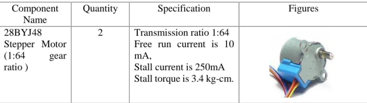
The mechanical components and their specifications are shown in

Table 2.1 while the rest of the components will be shown in electrical design section.

Table 2.1 : Mechanical components.

Component Name

Quantity Specification Figures

28BYJ48 Stepper Motor (1:64 gear ratio )

2 Transmission ratio 1:64 Free run current is 10 mA,

Stall current is 250mA Stall torque is 3.4 kg-cm.

(27)

3D printed Wheels 2 Diameter of wheel is 60mm, thickness of it is 3mm 3D printed Motor Brackets

2 This component was used to attach the motors on the base plate.

3D printed Chassis Base

1 This is the base for all components.

Ball Casters 1 This small ball caster uses a 9mm diameter metal ball.

(28)

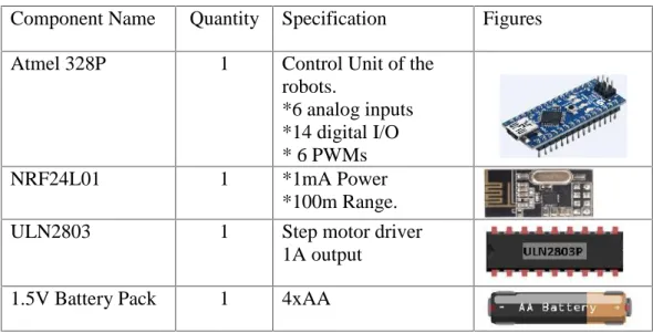
2.3 Design and Manufacturing of Mobile Robot Control Board

Each robot’s control board is based on 3 main components:



1 x Atmel 328P processor - Arduino Nano



1 x NRF24L01 RF connection module



1 x ULN2803 motor driver IC

Table 2.2 : Electrical components.

Component Name

Quantity

Specification

Figures

Atmel 328P

1 Control Unit of the

robots.

*6 analog inputs

*14 digital I/O

* 6 PWMs

NRF24L01

1 *1mA Power

*100m Range.

ULN2803

1 Step motor driver

1A output

1.5V Battery Pack

1 4xAA

Main power supply doesn’t require any voltage regulator since the battery pack is

within the operating range of all components. It can supply almost 5 hours of non-stop

fully operating functionality if 4AA alkaline batteries used in the pack.

Atmel328P, ULN2803 and NRF24L01 modules are mounted on a PCB and produced

as a single board for each robot.

(29)

Figure 2.1 : Control Board Schematic

2.4 NRF24L01 RF Communication Module

These modules consume very low power and are capable of operating almost 100m

range in an open area. RF modules on robots start operating as receivers, but PC side

RF main module begins operating as a transmitter. All robots change their modes from

receiver to transmitter and transfer “data received” signal to the main control board.

Main control board RF module changes to receiver mode to get “signal received”

confirmation from mobile robots. When the information from all robots confirmed,

main board sends another data to PC simulation, and the simulation interface updates

the pattern of Glider formation one step ahead.

Figure 2.2: NRF24L01 Module Pinouts

(30)

2.5 Communication Network with Multiple NRF24L01

We’ve created a small network between mobile robots and the main unit attached to

PC which communicates with the simulation interface. Main communication unit

sends required movement information to each robot one by one. After completed

pattern formations the simulation interface is updated.

Each NRF24L01 module keeps a unique address for communication and the main

control unit changes it’s address to connect with robots and transfer movement

information.

There are 5 different addresses used for each robot:



Swarm – Address name of 1st robot



nhytr – Address name of 2nd robot



bgtre

– Address name of 3rd robot



vfrew – Address name of 4th robot



cdewq – Address name of 5th robot

2.6 ULN2803A Motor Driver

The ULN2803A is a high-voltage, high-current Darlington transistor array. The

device consists of eight NPN Darlington pairs that feature high-voltage outputs with

common-cathode clamp diodes for switching inductive loads. The collector-current

rating of each Darlington pair is 500 mA. The Darlington pairs may be connected

in parallel for higher current capability [26].

(31)

2.7 28BYJ-48 Stepper Motors

A stepper motor is an electromechanical device which converts electrical pulses into

discrete mechanical movements. The shaft or spindle of a stepper motor rotates in

discrete step increments when electrical command pulses are applied to it in the proper

sequence. The sequence of the applied pulses is directly related to the direction of

motor shafts rotation. The speed of the motor shafts rotation is directly related to the

frequency of the input pulses and the length of rotation is directly related to the number

of input pulses applied. One of the most signiﬁcant advantages of a stepper motor is

its ability to be accurately controlled in an open loop system. This is a good reason

why we used 28BYJ-48 stepper motors.

Table 2.3 - 28BYJ-48 Stepper Motor Parameters [27]

Rated voltage ： 5VDC

DC Resistance ： 50Ω±7%(25

℃)

Number of Phase ： 4

In-traction Torque >34.3mN.m(120Hz)

Speed Variation Ratio ： 1/64

Self-positioning Torque >34.3mN.m

Stride Angle ： 5.625° /64

Friction torque : 600-1200 gf.cm

(32)

3. DESIGN AND IMPLEMENTATION OF SOFTWARE

3.1 Software of Mobile Robots

Each mobile robot is based on an Atmega328P processor. Programming Software is

chosen as Arduino IDE [28] which provides easy and sufficient environment for the

algorithm used.

Swarm robots gets movement data from Mega2560 module. They start as “receivers”

and when Mega2560 transfers movement data to the related robot, each robot sends a

uniqe character to Mega2560 module for “signal received” confirmation.

Swarm robots and Mega2560 communicates with different addresses. There are 5

different address names given to each robot initially:

Names

Robot Number

"Swarm"

1st Robot

"nhytr"

2nd Robot

"bgtre"

3rd Robot

"vfrew"

4th Robot

"cdewq"

5th Robot

Swarm robots program is given as a flowchart below:

Figure 3.1 – Swarm Robots Software Flowchart

Swarm robots have an indicator LED at their top side. This LED will turn to RED

while moving, turn to BLUE while in mid-pattern formation, and turn to GREEN when

(33)

3.2 Processing Simulation Interface

Real time Simulation of robots will be followed with a program interface created by

Processing [29]. The user will choose initial locations of robots by clicking to lattice

squares and related cell will turn to green to incidate the existance of robot in that cell.

Another step is to locate each robot on to choosen cells according to Simulation

interface. When the user hits “space bar” key, simulation and the data transfer will

start.

Following diagram (Figure 3.2) shows flowchart of Processing Simulation Program.

Figure 3.2 – Processing Simulation Flowchart

Some instructions about Simulation interface:



Click on any square to select/deselect it



Press “spacebar key” to pause/run simulation



Press “c” key clear screen and clear all selections

This simulation interface is based on “Processing/Topics/Cellular

Automata/GameOfLife.pde” program with some changes such as:



Serial communication with Mega2560 board (Simulation Line 49)

“myPort = new Serial(this, "COM17", 9600);”

(34)

Figure 3.3 – 4 different patterns of Glider Formation

Each pattern will be updated after simulation receives “g” from Mega2560 and sends

“g” as a confirmation of updated pattern.

Glider formation will keep moving acoording to GOL rules until the “spacebar” key

is pressed and the simulation is paused.



Cell size is changed due to a better visualization and required number of cells

as 7x7 cells.

(35)

3.3 Mega2560 Interface Board

Mega2560 board is used to communicate between Swarm Bots and the PC simulation.

When Mega2560 gets “start” signal from simulation, it sends data to SwarmBot1 and

receives a confirmation signal. It sends 2nd data to SwarmBot2 and receives another

confirmation signal back. If the signal is due to updated pattern then Mega2560 module

sends an update signal to simulation and waits for pattern updated confirmation signal

from PC side. This process goes on until all patterns are completed and the main cycle

starts again. The flowchart of Mega2560 program is as followed:

Figure 3.4 – Mega2560 Flowchart for Cycle1 Signal Order

When the 1st cycle is completed locations of Swarm Bots will be changed. Due to

relocation of robots, Mega2560 changes the order of signals for robots. Signal orders

for 1st and 2nd cycles can be given as in the following table:

Table 3.1 – Order of Signals for Swarm Robots through Cycle1 and Cycle2

Signal Orders of Robots for Cycle 1

Signal Orders of Robots for Cycle 2

1st

4th

3rd

5th

2nd

3rd

2nd

5th

2nd

1st

2nd

4th

(36)

According to the Table 3.1 it is clear that “Robot1  Robot3” and

“Robot4Robot5” changes their addresses after each cycle completed. Locations

of these robots changes after each cycle and Mega2560 switches between two signal

orders. This method can be better organized with different coding.

Cycle2 signal re-order flowchart can be given as followed:

Figure 3.5 – Mega2560 Flowchart for Cycle2 Signal Order

Mega2560 module works as a communication way between Swarm Robots and the

simulation interface. The functionality of Mega2560 can be done by using Atmega

328P processor based Arduino Nano board.

(37)

4. TEST RESULTS OF COMPLETE SYSTEM

Our Swarm Robots are designed to play “Game Of Life” algorithm in “Glider”

formation. There are two cycles follow each other for complete pattern and relocation

of swarm robots. We can represent how complete system works as followed:

Figure 4.1 – Complete System Diagram

Cycle1 and Cycle2 are almost the same except names of 4 robots swicthes between

13 and 45. This is required due to relocation of robots and the main signal

should be sent according to new locations of robots. After they return to their initial

locations, glider formation will be re-created, and so on.

These are the followed patterns and the pictures of robots while they follow Glider

formation.

(38)

(a)

(b)

Figure 4.2 Cycle1 Pattern1 (a) Diagram (b) Realization Picture

(a)

(b)

Figure 4.3 Cycle1 Pattern2 (a) Diagram (b) Realization Picture

(39)

(a)

(b)

Figure 4.5 Cycle1Pattern4 (a) Diagram (b) Realization Picture

(a)

(b)

Figure 4.6 Cycle2 Pattern1 (a) Diagram (b) Realization Picture

(40)

(a)

(b)

Figure 4.8 Cycle2 Pattern3 (a) Diagram (b) Realization Picture

(a)

(b)

(41)

After this step, all robots will be returned to their initial positions and Cycle1 restarts.

This two cycles will continue until the simulation stopped.

(a)

(b)

Figure 4.10 Cycle1 Pattern1 (a) Diagram (b) Realization Picture

The movement precision of Swarm robots is enough good to create each pattern. Two

cycles can be completed without leaving the boundaries of squared ground. This

precision is based on 28BJY-48 stepper motors.

Movement speeds of swarm robots is chosen maximum speed of stepper motors.

Precision is kept even with the highest speed of motors. Total movement duration of

each pattern is given in the table below.

Table 4.1 – Movement time of robots for each pattern creation

Formation Time of Cycle1 Patterns (s) Formation Time of Cycle2 Patterns (s)

1

21

1

22

2

21

2

21

3

33

3

34

4

25

4

24 As we can see that precision of robots are good enough as timing. There are some

mechanical disturbances on robots while they move. Especially during rotations to left

(42)

remember robots 1-3 and 4-5 switches locations and they show different movements

for each cycle. This change causes the minor time difference between cycles for

pattern1 and pattern3 formations as in the table. Robot2 doesn’t show any time

difference between two cycles because it follows the same movements for both cycles.

(43)

5. CONCLUSION

Swarm robotics is one of the most interesting areas of advancing technology. Benefits

of swarm robotics will be huge on human life and production abilities. We aimed to

contribute to the advancements of swarm robotics including another very interesting

area which is Cellular Automata based Glider Formation Algorithm.

Gliders are very interesting formations of CA.Our main purpose is to create a swarm

group that demonstrates Game of Life and create Glider formation on a 2D squared

lattice. Production of robots are completely done from scratch. Mechanical design,

circuit production and coding are all done step by step.

Simulation and Swarm Robots were successfully worked and tested. Simulation

program is not designed very functional because it requires only realization of swarm

movements as expected. It is designed only to show pattern updates and pause/stop

controls of swarm group.

There are a lot of future advencements can be added to our Glider Swarm system. Such

as;



Desired path can be chosen by users from simulation interface and robots can

follow the chosen path.



Number of robots can be increased and different Cellular Automata formations

can be trained with the same system. This will be very interesting to see how

different CA formations will be realized by swarm robots.



One of the most important improvement will be to include sensors to our

swarm robots. Sensors are not needed with this Glider formation but if swarm

robots has to move at the same time to create each pattern and they start moving

at the same time, then sensor information will be crucial to avoid collisions

between robots.



Another interesting future improvement would be to try swarm system

including sensors and obstacles on the grid. These obstacles will be avoided by

robots while they create glider formations. Whenever a robot crosses an

obstacle it will inform main simulation interface and all other robots of swarm

group will be aware of already discovered obstacle on the same grid. With this

method, swarm robots can handle very important tasks such as “rescue”,

“search”, and “mapping”. This future improvement will require location

information to be carried for each robot individually and the simulation

interface will follow each robots location simultanously.

(44)

system. Each robot will keep it’s movement information and after it completes

its movement, it will inform the next robot to continue to create glider

formation. Mega2560 is not required in this case because simulation interface

will not be needed to control the swarm but robots will communicate with each

other. This system can be implemented with some new codes to robot group

without Mega2560 and Processing interface.

This work we’ve implemented as hardware, software and simulation interface was a

success to realize Glider pattern “Game of Life” algorithm applied Swarm robotics. It

needs better mechanical production, however it is enough good to observe desired

patterns and simulation at the same time as planned.

(45)

REFERENCES

1. Arkin, R.C.: Behavior-based robotics. MIT Press (1998)

2. Zhang, Y., Fattahi, N., Li, W.: Probabilistic roadmap with self-learning for path

planning of a mobile robot in a dynamic and unstructured environment. In:

Mechatronics and Automation (ICMA), pp. 1074–1079 (2013)

3. Ramer, C., Reitelshofer, S., Franke, J.: A robot motion planner for 6-DOF industrial

robots based on the cell decomposition of the workspace. In: 2013 44th

International Symposium on Robotics (ISR), pp. 1–4 (2013)

4. Jianjun, Y., Hongwei, D., Guanwei, W., Lu, Z.: Research about local path planning

of moving robot based on improved artificial potential field. In: Control and

Decision Conference (CCDC), pp. 2861–2865 (2013)

5. Mitchell, M.: Computation in cellular automata: A selected review. Non-standard

Computation, 385–390 (1996)

6. Oliveira, G., Martins, L.G.A., de Carvalho, L.B., Fynn, E.: Some investigations

about synchronization and density classification tasks in one-dimensional and

two-dimensional cellular automata rule spaces. Electronic Notes in Theoretical

Computer Science 252,121–142

7. Behring, C., Bracho, M., Castro, M., Moreno, J.A.: An Algorithm for Robot Path

Planning with Cellular Automata. In: Proc. of the 4th Int. Conf. on Cellular

Automata for Research and Industry, pp. 11–19 (2000)

8. Soofiyani, F.R., Rahmani, A.M., Mohsenzadeh, M.: A Straight Moving Path

Planner for Mobile Robots in Static Environments Using Cellular Automata. In: Int.

Conf. on Computational Intelligence, Communication Systems and Networks, pp.

67–71 (2010)

9. Rosenberg, A.: Cellular ANTomata. Paral. and Distributed Processing and

Applications,78–90 (2007)

10. Cyberbotics.

Webots

7:

robot

simulator

(2013),

http://www.cyberbotics.com/overview

11. E-puck Education Robot, http://www.e-puck.org

12. Akbarimajd, A., Lucas, C.: A New Architecture to Execute CAs-Based

Path-Planning Algorithm in Mobile Robots. In: IEEE Int. Conf. on Mechatronics, pp.

478–482 (2006)

13. Akbarimajd, A., Hassanzadeh, A.: A novel cellular automata based real time path

planning method for mobile robots. Int. Journal of Engineering Research and

Applications (2011)

14. Ioannidis, K., Sirakoulis, G.C., Andreadis, I.: A Cellular Automaton

Collision-Free Path Planner Suitable for Cooperative Robots. In: Panhellenic Conf. on

Informatics (2008)

15. Ioannidis, K., Sirakoulis, G., Andreadis, I.: Cellular ants: A method to create

collision free trajectories for a cooperative robot team. Robotics and Autonomous

(46)

16. Shu, C., Buxton, H.: Parallel path planning on the distributed array processor.

Parallel Computing 21(11), 1749–1767 (1995)

17. Marchese, F.: A reactive planner for mobile robots with generic shapes and

kinematics on variable terrains. In: Proc. Advanced Robotics, ICAR 2005, pp. 23–

30 (2005)

18. Tzionas, P., Thanailakis, A., Tsalides, P.: Collision-free path planning for a

diamond shaped robot using two-dimensional CA. IEEE Trans. on Rob. and

Automation (1997)

19. https://cs.stanford.edu/people/eroberts/courses/soco/projects/2008-09/modeling-natural-systems/boids.html

20. T. Fukuda and Y. Kawakuchi. Cellular robotic system (CEBOT) as one of the

realization of selforganizing intelligent universal manipulator. In Proc. of IEEE Int'l

Conf. on Robotics and Automation.

21. Atyabi, A., Phon-Amnuaisuk, S., and Ho, C.K. (2010). Applying area extension

PSO in robotic swarm. Journal of Intelligent and Robotic Systems.

22. Fredslund, J. and M.J. Mataric, A general algorithm for robot formations using

local sensing and minimal communication. Robotics and Automation, IEEE

Transactions on, 2002. 18(5): p. 837-846.

23. Turgut, A.E., et al., Self-organized flocking in mobile robot swarms. Swarm

Intelligence, 2008. 2(2-4): p. 97-120.

24. Bahçeci, E. Evolving aggregation behaviors for swarm robotic systems: A

systematic case study. in Swarm Intelligence Symposium, 2005. SIS 2005.

Proceedings 2005 IEEE. 2005. IEEE.

25. J.L. Schi

ﬀ, Introduction to Cellular Automata, Wiley , February 2008.

26. https://www.sparkfun.com/datasheets/IC/uln2803a.pdf

27. https://arduino-info.wikispaces.com/SmallSteppers

28. https://www.arduino.cc/en/

(47)

APPENDICES

APPENDIX A: The control code of Swarm Robots

APPENDIX B: The code of Mega2560 Communication Unit

APPENDIX C: The code of Processing Simulation

APPENDIX A:

/*

* Kasım Gül

* Master Thesis 2017.08.18 - İzmir Katip Çelebi Üniversitesi

* Glider Formation Game of Life Algorithm applied Swarm Robots

*

* Arduino Nano v.3 and Arduino 1.8.0 IDE

*/

// SPI(nRF24L01) commands

#define READ_REG 0x00 // Define read command to register

#define WRITE_REG 0x20 // Define write command to register

#define RD_RX_PLOAD 0x61 // Define RX payload register address

#define WR_TX_PLOAD 0xA0 // Define TX payload register address

#define W_ACK_PAYLOAD 0xA8 // pipe buna eklenecek

#define FLUSH_TX 0xE1 // Define flush TX register command

#define FLUSH_RX 0xE2 // Define flush RX register command

(48)

#define REUSE_TX_PL 0xE3 // Define reuse TX payload register command

#define ACTIVATE 0x50 //

#define NOP 0xFF // No Operation, might be used to read status register

//---#define RX_DR 0x40 //data geldi biti

#define TX_DS 0x20

#define MAX_RT 0x10

//---// SPI(nRF24L01) registers(addresses)

#define CONFIG 0x00 // 'Config' register address

#define EN_AA 0x01 // 'Enable Auto Acknowledgment' register address

#define EN_RXADDR 0x02 // 'Enabled RX addresses' register address

#define SETUP_AW 0x03 // 'Setup address width' register address

#define SETUP_RETR 0x04 // 'Setup Auto. Retrans' register address

#define RF_CH 0x05 // 'RF channel' register address

#define RF_SETUP 0x06 // 'RF setup' register address

#define STATUS

0x07 // 'Status' register address

#define OBSERVE_TX 0x08 // 'Observe TX' register address

#define CD 0x09 // 'Carrier Detect' register address

#define RX_ADDR_P0 0x0A // 'RX address pipe0' register address

#define RX_ADDR_P1

0x0B // 'RX address pipe1' register address

#define RX_ADDR_P2 0x0C // 'RX address pipe2' register address

#define RX_ADDR_P3 0x0D // 'RX address pipe3' register address

#define RX_ADDR_P4 0x0E // 'RX address pipe4' register address

#define RX_ADDR_P5 0x0F // 'RX address pipe5' register address

#define TX_ADDR 0x10 // 'TX address' register address

(49)

#define RX_PW_P1 0x12 // 'RX payload width, pipe1' register address

#define RX_PW_P2 0x13 // 'RX payload width, pipe2' register address

#define RX_PW_P3 0x14 // 'RX payload width, pipe3' register address

#define RX_PW_P4 0x15 // 'RX payload width, pipe4' register address

#define RX_PW_P5 0x16 // 'RX payload width, pipe5' register address

#define FIFO_STATUS 0x17 // 'FIFO Status Register' register address

#define DYNPD 0x1C //

#define FEATURE 0x1D //

#define CE 0 // Chip Enable Activates RX or TX mode

#define CSN 1 // SPI Chip Select ,Slave Enable signal, controlled by master

#define SCK_PIN 13 // SPI Clock,controlled by master

#define MOSI_PIN 11 // SPI Master Data Output,Slave Data Input

#define MISO_PIN 12 // SPI Master Data Input, Slave Data Output, with tri-state option

//---#define TX_ADR_WIDTH 5 // TX/RX adres genişliği

#define TX_PLOAD_WIDTH 30 // 30 RX/TX gönderme/alma bayt sayısı payload

int i; //used for islemler() function

char data;

int buzzerPin=10; //Buzzer to implement short sounds for swarm robots

//Names and data transmission channels defined here

char pipe0[] = "Swarm"; //Robot1 name;

char pipe1[] = "nhytr"; //Robot2 name;

char pipe2[] = "bgtre"; //Robot3 name;

char pipe3[] = "vfrew"; //Robot4 name;

char pipe4[] = "cdewq"; //Robot5 name;

(50)

char pipe0_adresi[10];

char pipe1_adresi[10];

char pipe2_adresi[10];

char pipe3_adresi[10];

char pipe4_adresi[10];

unsigned char rx_buf[35] = {0}; // fill with 0s

char tx_buf[35];

char isim[20];

unsigned char X;

char veri;

int Steps = 0;

int bekle=1000;

boolean Direction1 = true;// Motor1 direction

boolean Direction2 = true;// Motor2 direction

unsigned long last_time;

unsigned long currentMillis ;

int steps_left;

long time;

int kalinanYer=0;

int donerken=1880;

int ilerle=4430;

bool RF_mod=true;

int RPIN = A3;

int GPIN = A4;

int BPIN = A5;

(51)

void pulse_CSN()

{

digitalWrite(CSN, HIGH);

delayMicroseconds(20);

digitalWrite(CSN, LOW);

}

//This function allows us to use names for Swarm robots with more than 5 characters

void isim_ayarla( char *pBuf)

{

byte i; byte uzunluk=0; byte orta=0;

memset(isim,0,sizeof(isim)); //CLEAR

uzunluk=strlen(pBuf); // verdiğimiz pipe isim uzunluğunu bul

orta=uzunluk/2;// "adres" dizisinin ortasını bul

//"pBuf" dizisinin en sağından 2 karekteri "isim" dizisine al (Ters al)

isim[0]=pBuf[uzunluk-1];

isim[1]=pBuf[uzunluk-2];

isim[2]=pBuf[orta]; // "pBuf" dizisinin ortasından bir karekteri "isim" dizisine ekle

isim[3]=pBuf[1];

isim[4]=pBuf[0];

strcpy(pipe0_adresi,isim ); //"isim" dizisini "pipe0_adresi" dizisine kopyala

}

//---// NRF2401 in bağlı olduğu pinlerin giriş çıkış durumunu ayarlar

void NRF_Init(void)

{

pinMode(CE, OUTPUT);

pinMode(SCK_PIN, OUTPUT);

(52)

pinMode(CSN, OUTPUT);

pinMode(MOSI_PIN, OUTPUT);

pinMode(MISO_PIN, INPUT);

digitalWrite(CE, 0); // chip enable

digitalWrite(CSN, 1); // Spi disable

}

// unsigned char bir bayt nRF24L01 e yazar,ve unsigned char bir bayt okur döndürür

unsigned char SPI_RW(unsigned char Byte)

{

unsigned char i;

for(i=0;i<8;i++) // output 8-bit

{

if(Byte&0x80)

{

digitalWrite(MOSI_PIN, 1);

}

else

{

digitalWrite(MOSI_PIN, 0);

}

digitalWrite(SCK_PIN, 1);

Byte <<= 1; // shift next bit into MSB..

if(digitalRead(MISO_PIN) == 1)

{

Byte |= 1; // capture current MISO bit

}

(53)

}

return(Byte); // return read unsigned char

}

unsigned char SPI_RW_Reg(unsigned char reg, unsigned char value)

{

unsigned char status;

digitalWrite(CSN, 0); // CSN low, init SPI transaction

status = SPI_RW(reg); // select register

SPI_RW(value); // and write value to it..

digitalWrite(CSN, 1); // CSN high again

return(status); // return nRF24L01 status unsigned char

}

unsigned char SPI_Read(unsigned char reg)

{

unsigned char reg_val;

digitalWrite(CSN, 0); // CSN low, initialize SPI communication...

SPI_RW(reg); // Select register to read from..

reg_val = SPI_RW(0); // ..then read register value

digitalWrite(CSN, 1); // CSN high, terminate SPI communication

return(reg_val); // return register value

}

unsigned char SPI_Read_Buf(unsigned char reg, unsigned char *pBuf, unsigned char bytes)

{

unsigned char status,i;

digitalWrite(CSN, 0); // Set CSN low, init SPI tranaction

status = SPI_RW(reg); // Select register to write to and read status unsigned char

for(i=0;i<bytes;i++)

(54)

{

pBuf[i] = SPI_RW(0); // Perform SPI_RW to read unsigned char from nRF24L01

}

digitalWrite(CSN, 1); // Set CSN high again

return(status); // return nRF24L01 status unsigned char

}

unsigned char SPI_Write_Buf(unsigned char reg, char *pBuf, unsigned char bytes)

{

unsigned char status,i;

digitalWrite(CSN, 0); // Set CSN low, init SPI tranaction

status = SPI_RW(reg); // Select register to write to and read status unsigned char

for(i=0;i<bytes; i++) // then write all unsigned char in buffer(*pBuf)

{

SPI_RW(*pBuf++);

}

digitalWrite(CSN, 1); // Set CSN high again

return(status); // return nRF24L01 status unsigned char

}

void NRF_SeTxMode(void)

{

digitalWrite(CE, 0);

//PWR_UP=1, enable 1 bayt CRC,TX,MAX_RT & TX_DS ve RX_DR

SPI_RW_Reg(WRITE_REG + CONFIG, 0x0A);

SPI_RW_Reg(WRITE_REG + EN_AA, 0x01); //sadece pipe0 ACK göndersin

SPI_RW_Reg(WRITE_REG + SETUP_RETR, 0xFF); //

SPI_Write_Buf(WRITE_REG + TX_ADDR, isim, TX_ADR_WIDTH); // Writes TX_Address

SPI_Write_Buf(WRITE_REG + RX_ADDR_P0, isim, TX_ADR_WIDTH);

(55)

SPI_RW_Reg(WRITE_REG + EN_RXADDR, 0x01);//Sadece pipe 0 ı enable et TAMAM

SPI_RW_Reg(WRITE_REG + RF_CH, 2); //RF kanal 2

SPI_RW_Reg(WRITE_REG + RF_SETUP, 0x07); ////data rate = 1MB 0 dBm 1 MW

digitalWrite(CE, 1);

}

void NRF_Send(unsigned char *buf_tx)

{

SPI_RW_Reg(FLUSH_TX,0); // Clear TX Buffer

SPI_RW_Reg(WRITE_REG+STATUS,0xff);//Clear interrupt flags

RX_DR,TX_DS,MAX_RT

//Write data to NRF24L module

SPI_Write_Buf(WR_TX_PLOAD,tx_buf,TX_PLOAD_WIDTH);

}

//If ACK signal detected return1 else return0

unsigned char NRF_CheckAck(void)

{

unsigned char sta;

sta = SPI_Read(STATUS); // Serial.println(sta);

if(sta & TX_DS) //BIT5

{

return(1);

}

else {return(0);}

}

void NRF_SetRxMode(void)

{

digitalWrite(CE, 0);

(56)

SPI_RW_Reg(WRITE_REG + EN_AA, 0x01);//Sadece pipe 0 ACK göndersin

SPI_RW_Reg(WRITE_REG + SETUP_RETR, 0xFF);

SPI_RW_Reg(WRITE_REG + EN_RXADDR, 0x01);

SPI_RW_Reg(WRITE_REG + SETUP_AW, 0x03);

SPI_RW_Reg(WRITE_REG + RF_SETUP, 0x07);// Set to: 1Mbps 0dBm 1mW

SPI_RW_Reg(WRITE_REG + RX_PW_P0,TX_PLOAD_WIDTH);

SPI_RW_Reg(WRITE_REG + RF_CH,2);

SPI_Write_Buf(WRITE_REG + TX_ADDR, pipe0_adresi, TX_ADR_WIDTH);

SPI_Write_Buf(WRITE_REG + RX_ADDR_P0, pipe0_adresi, TX_ADR_WIDTH);

SPI_RW_Reg(WRITE_REG + CONFIG, 0x7B);

}

unsigned char NRF_Receive(unsigned char *buf_rx)

{

unsigned char genel;

unsigned char sta = SPI_Read(STATUS);// Serial.println(sta);

if(sta & RX_DR)// STATUS un 6.biti (RX_DR Data hazır flag) test et H ise

{

genel=sta & 0x0E;

genel=genel>>1; // Shift 1 bit to right

//Read received data and store in "rx_buf" array

SPI_Read_Buf(RD_RX_PLOAD, rx_buf, TX_PLOAD_WIDTH);

SPI_RW_Reg(FLUSH_RX,0); // Clear RX buffer

SPI_RW_Reg(WRITE_REG+STATUS,0xff);

return 1; }

else

(57)

void setup()

{

for(int pin=2;pin<11;pin++)

{

pinMode(pin, OUTPUT);

}

pinMode(RPIN, OUTPUT);

pinMode(BPIN, OUTPUT);

pinMode(GPIN, OUTPUT);

NRF_Init();// IO portları ayarla

digitalWrite(RPIN, 0);

digitalWrite(GPIN, 1);

digitalWrite(BPIN, 0);

}

void loop()

{

while(true)

{

isim_ayarla(pipe0); // Swarm adresli robot olarak başlayacak

NRF_SetRxMode(); //Alıcı moduna ayarla

delay(50);

if(NRF_Receive(rx_buf))//Eğer data gelmişse gir (gelen Data şimdi "rx_buf" ta)

{

if(rx_buf[0]=='k') //this condition is used to avoid complication between Mega2560 and Robot1