Markov modulated periodic arrival process offered to an ATM multiplexer

(1)

Markov Modulated Periodic Arrival Process Offered

to

an

ATM Multiplexer

Nail Akar and Erdal Arikan

Electrical and Electronics Eng. Dept.

Bilkent University,

06533

Ankara, Turkey

ABSTRACT

When a superposition of on/off sources is offered to a deterministic server, a particular queueing system arises whose analysis has a significant role in ATM based networks. Periodic cell generation during active times is a major feature of these sources. In this paper a new an- alytical method is provided to solve for this queueing system via an approximation to the transient behavior of the n D / D / l queue. The solution t o the queue length distribution is given in terms of a solution to a linear differential equation with variable coefficients. The technique proposed here has close similarities with the fluid flow approximations and is amenable to extension for more complicated queueing systems with such correlated arrival processes. A numerical example for a packetized voice multiplexer is finally given to demonstrate our results.

Introduction

The Asynchronous Transfer Mode (ATM) is the preferred transfer mode for the Broadband ISDN (B-ISDN). The core of an ATM network is “asynchronous multiplexing” on the basis of which transmission links and switching devices are shared by different virtual connections. Information is transmitted in the form of constant length packets, called “cells”. Since ATM has the potential to improve bandwidth efficiency via the use of statistical multiplexing of variable bit-rate sources, characterization of a traffic stream belonging to a particular connection turns out to have an important role. In fixed bit rate coding schemes, sources emit cells periodically with a fre- quency determined by their bit rate. On/off sources emit cells periodically during activity (on) times alternating with silence (off) times during which there is no cell generation. These two periods are in general of variable length. In this paper, we focus on a queueing system in which several on/off sources with an identical period share a buffer of infinite size. Given the number of sources and the associated traffic parameters, we are interested in the probability distribution function of the buffer content. A 2-state continuous-time Markov chain model (see Figure 1) will be used to describe the aforemen- tioned traffic stream. In this model, the silence times and

x

P

Figure 1: 2-state Markov model for an on/off source the activity times are exponentially distributed with means 0-7803-0917-0/93$03.00 Q 1993 IEEE

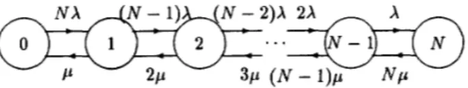
1/X and l/p, respectively. This 2-state model can be ex- tended to construct an N-state Markov chain to describe the superposition process of N on/off sources (see Figure 2). The

Figure 2: Birth-death model for the superposition of N on/off sources

state of the Markov chain is defined to be the number of ac- tive sources. In an arbitrary state, say n , of the Markov chain whose state holding time is exponentially distributed with pa- rameter U,,

=

( N - n ) X + n p , n sources independently transmit cells with an identical period. In general, we call the arrival process as a Markov modulated periodic arrival process.

The arrival process associated with the superposition pos- sesses two kinds of correlations:

0 negative correlations of arrivals in successive time slots

due to the periodic nature of cell transmissions,

0 positive correlations among the average arrival rates in

successive periods of length greater than the intercell times of the multiplexed sources.

There are various approaches proposed in the literature which take account of these correlation effects in the performance analysis of the queueing system [l]. One basic approach is using fluid flow models. These models approximate the cell arrival and service process by continuous arrival and depar- ture of a fluid. The superposition of a finite number of on/off fluid sources is considered in [2] for which the authors give a computationally efficient algorithm to evaluate the buffer occupancy distribution. However, the model does not give accurate results for low to moderate traffic when cell layer contention dominates over burst layer contention. This is be- cause the first type of correlations cannot be captured by fluid flow models. The model and technique proposed in [2] is further applied to the finite buffer case in [3] to solve for the cell loss rate which is a critical performance measure in ATM networks.

For an accurate analysis of an ATM multiplexer, the negative correlation between cell interarrival times should also be taken into consideration. Actually, when the instantaneous arrival rate is less than the link rate, the queueing system

(2)

behaves like the so-called n D / D / 1 queue: a superposition of independent periodic sources (n sources) with an identical period but with random phase feeds a constant service time buffer. This queue is investigated in [4], [5] to find the steady- state distribution of the queue length. Different periods are also allowed in [SI where accurate approximate formulas for the queue length distribution are derived.

In our queueing model that considers a Markov modulated periodic arrival process as input to the multiplexer, tlhe transient behavior of the n D / D / l queue has a significant role. The focus of this paper is on the derivation of a relationship between fluid sources and periodic sources, arrival rates of which are Markov modulated in the same manner, through an approximation of the transient behavior of the n D / D / l

queue. This approximation is mainly based on an interpolation of the queue length whose distribution is known at certain epochs. The solution for the overall problem is then reduced to the solution of a linear differential equation with variable coeficients whereas in fluid flow approximations the corresponding equation is simply linear with constant coefficients.

A numerical example is finally given in the context of a packetized voice multiplexer.

Problem Formulation and Analysis

The method used in solving for the steady-state distribution of the queue length for the Markov modulated periodic arrival case is composed of two main stages. Tlie first stage consists of an approximation to the transient behavior of the 7 i D / D / 1

queue in a continuous-time framework. In the second stage, we extend our results for the nD/D/1 queue to solve for the cont,inuous-time Markov model which characterizes the input traffic.

Let us first consider the case when the number of active sources ( T I ) is fixed. In our queueing model, we assume that the t,ime axis is slotted where each time slot is as long as the transmission time of a cell. The cells arriving to the queue are served on a first-conie-first-serve basis and the queue has infinite size. The n active sources each transinit fixed length cells with a period of R slots. independently of each other. I n an arbitrary frame of R slots, each input source’s cell can be in any of these R slots with equal probability. Tlie peak source ra1.e in cells/sec is denoted by P and the service rate of the buRer is denoted by C , which actually equals to P R cells/sec. Wit,liout loss of generality, we assume that the departures take place at the beginning of slots, and arrivals during slots. Let us assume a stable queue ( 7 1

<

R ) for the time being and define the following random variables

Qk = queue length at t,he end of k t h dot,

a k = number of arrivals in the

**k*“**

slot,.

The queueing strategy is the following:

Q k

=

{

O‘ i f k = O

max(Qk-1 - 1 , o )

+

ak if

k >

0

By iteration on k , one can check using algebraic manipulations that

Q R = max(Q,, QO

+

71 - R ) ₍₁₎

where the random variable Qn is defined via R

The cumulative distribution function for the random variable Qn is expressed by the following summation [5]

where q is the largest integer smaller than q and q

5

n

-

1. In order to obtain the queue length evolution equations for ti

<

R , we iterate on equation (1) on an R-slot basis so that by periodicity of arrivals we have

&kR = max(Q,, Q o

+

k ( n - R ) ) , k

=

1,2,. .

.

(4)

There is, in fact, a strong interconnection between periodic models and fluid flow models. In the latter models, information is assumed to arrive uniformly to the multiplexer and the server similarly removes information from the queue, in a continuous manner. The computational tractability and buffer size independent solvability of fluid flow approximation techniques suggest a further study of this interconnection.

If we define Q ( t ) as the queue length at time t , the fluid flow approximations suggest that

[a]:

Q ( t )

= max(0,

QO

+

( P P I - 6)t). ₍₅₎

Note the noninteger values that Q ( t ) may take due to the

absence of the concept of packetization in fluid models. There are two major differences between the expressions (4) and (5). The first term associated with the short term fluctuations of the quene length is the random variable Qn in the periodic model whereas it equals zero in the fluid model. This is why the fluid flow models do not give accurate results in light to moderate traffic when several on/off sources are multiplexed on a common link. This deficiency belonging to fluid models has been mentioned by several authors [7], [8]. The second term associated with the dynamical behavior of the queue length in (5) is just a linear interpolation of the corresponding term in (4).

For the overload states, since the probability that the queue length is zero at some time epoch is negligible, fluid flow approximation gives accurate results in the analysis of the transient response of the queue. Taking (4) as our key equality, our approach is mainly based on interpolating the second term as in (5) while preserving the first term, Qn, which captures the short term fluctuations in the cell layer.

In regard of these observations, we approximate Q ( t ) by

(6) max(Q,,Qo

+

( P n - C ) t ) , 71

<

R

0

+

( P n

-

C)l, 71

2

R

Q ( t ) =

{

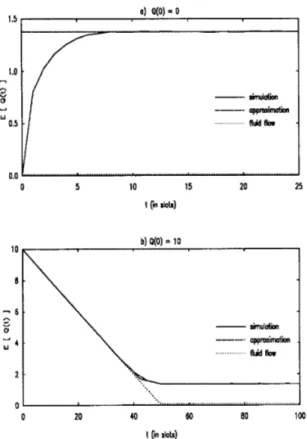
Q

The accuracy of this approximation for the average queue length in an n D / D / l queue is examined in Figure 3 and compared with simulation results and fluid flow approximations. 784

(3)

0.5 0.0 0 5 10 15 20 25 I (in slots)

’I

lo

-

simUlo(0n approximatan . fluid Ror ...

zt

0 1 , .. ... 0 20 40 bo 80 100 I (in slats)

Figure

3:

Comparison of approximations for the expected value of the queue length for the case R

=

10 and n

=

8 .

For the case R

=

10 and n

=

8 , we allow the queue start with two different initial levels.

The major observation is that, the approximation (6) is accurate when the initial buffer content is not in the vicinity of zero. Even in this case, the approximation is able to track the simulation curve after the queue length reaches its stead,y- state distribution. Better results compared with fluid flow approximations are obtained irrespective of the initial buffer content. The fundamental approximation in (6) will now be used to derive formulas for the queue length distribution when the number of active sources is changed according to the state of the birth-death model.

Let us now consider the traffic model in Figure 2 and con-

centrate on a particular state ( n , 0

<

n

5

N ) of the Markov chain. Let

X ( t )

be the buffer content and S(t) be the state of the Markov chain a t time

t .

Also let 7rn be the station-

ary probability of n sources being active. We then define the following stationary probabilities (as t + 03, At -+ O+):

r b ( n , z)

=

P r { X ( t )

5

zlS(t

+

A t ) = n ,

S ( t )

#

S(t

+

A t ) )

and

F e ( n , z)

=

P r ( X ( 1 )

5

zlS(t

+

A t )

#

S(t), S ( t ) = n } .

Note that S ( t ) is the state of a continuous-time Markov chain; given S ( t ) , the buffer content X ( t ) will be independent of

S(t

+

A t ) . This fact yields

Fe(n, z)

=

P r { X ( t )

<

xIs(t)

=

n } .

To interpret, Fb(n, z) is the equilibrium probability that the queue length is less than 2 given th2t a state transition to state n is about to occur. Similarly, F e ( n , z) is the stationary probability that the queue length is less than z given that a state transition from state n is about t o occur. In other words, we observe the queue length a t the time epochs when state transitions occur and henceforth define the corresponding random variables. We then define Fb(n, z)

=

7rnFb(n, z)

and F e ( n , Z)

=

T n F e ( n , z).

Each time the Markov system changes a state we assume a complete phase randomization of all the sources whereas for the original system an active source’s phase is independent of the other sources’ state transitions. With this assumption, the station_ary queue length at the moment of state transition to n and Qn become independent. By exploiting the approximation ( 6 ) and with the above assumption one obtains

A

where

the subscript f denotes the fluid flow term and U(.) is the unit step function. We can then write down the differential equation that governs F j ( n , z) for z

>

0:

(8)

Now letting p ( m , n ) be the state transition rate from state m to state n , we relate Fa(n, 2)’s to

Fe(.,

2 ) ’ s . It is not difficult to show by using the balance equations of the Markov chain that

bnFb(n, 3)

=

p ( m , n ) F e ( m , z). (9)

m#n

Combining(7), (8), and (9), we finally obtain the following differential equations for F j ( n , z)’s:

and

A

In the-above equations, Q m ( z )

=

1, Vz

>

0 , m

2

R . If the term Q n ( z ) is taken as unity V n , n

=

O , l , .

...

N , then the above equations are equivalent to the fluid flow equations [2].

(4)

F j ( x ) =

where the N x N matrix A ( E ) is determined through asuitable arrangement of the differential equations in (10). Actually,

A ( t ) = A i , x E [ i , i + l ) ,

i

E 2+, 0

5

i

5

R - 2 , and

A ( z ) = A , z E [R - 1,m)

for some appropriate constant matrices Ai's and A , _due to the piecewise constant structure of the distributions Qn(.)'s.

Given the initial condition F j ( O ) , the differential equation ( 1 1) has a unique continuous solution described by

FJ(c)

=

exp(Ai(z - i ) ) F j ( i ) , 1: E [ i , i + I], 0

5

i

5

R - 2, (12)

and

F j ( z )

=

exp(A(z - ( R - l ) ) ) F j ( R - l ) , E

2

R - 1 . (13)

In order to find the initial condition, we make use of the following observations:

-

F f ( W

-

Ff

(11

x)

F j ( R - 1 , z) I F f ( R + 1,z)

-

Fj(N,X)

-

For n

>

R , the queue is always increasing, so the queue length cannot be zero. Therefore, F j ( i i , 0)

=

0 for n

>

R.

The matrix A is, i n fact, equivalent to the stale matrix in fluid flow models, therefore it is known to have R - 1 positive real eigenvalues, N

-

R negative real eigenvalues and an eigenvalue at the origin. In order for the solution not to blow up as x 4 za, no positive (unstable) modes

of A should be excited by the choice of F j ( 0 ) . The behavior of F j ( i i , E ) as z 4 CO is easy to write:

Fj(?i,00) = K,, V71, 0

5

7 1

5

N .

Now, let zi be a stable eigenvalue of A and

4,

be its corre- sponding right eigenvector. Then, by observation 2 and (13), the solution to F j ( x ) can be written in the form

N - R F ~ ( x ) = ~ j ( m )

+

exp(=i(c

-

R

+

l ) ) / i i @ i , z

2 R

- I i = l which yields N - R ' F ~ ( R - 1) = I ~ ~ ( c o )

+

I L i 4 j l (14) i= 1

where p i ' s are coefficients to be determined. The relationship between F j ( 0 ) and F j ( R - 1) now needs to be established. Using (12), one can write

R - 2 F j ( R - 1 )

=

Z F j ( 0 )

Besides, by observation 1, F j ( 0 ) is in the form

L J

where f is of size R x 1 . Cornbining (14) and (15), one can solve for pi's and f , and thus the initial condition F j ( 0 )

through a linear matrix equation of size N . Having found the initial condition, the solutions given in (12) and (13) com- plete our description of the queue length distribution through (7). The essential difference between the method presented here and computations encountered in solving the fluid flow models is the calculation of the linear operator 2 in (15).

The overall cdf of queue length is the sum of the individual elements F,(n, E ) :

Pr(queue length

5

z)

=

Fe(71, x). n = O

Numerical Example

We consider a packetized voice system with voice peak rate

32 Kbits/sec., R

=

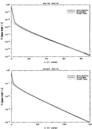
10, mean active period 353 ms. and meail silent period 650 ms. The packets are 64 bytes and

the packet transmission time is 1.6 nis. Within an active period, cells from an individual voice source are transmitted in a periodic manner, each source's phase being uniform between 0 and 9. In Table 1 , the mean waiting time in the queue with respect to the nuniber of voice sources by our analysis method and the fluid flow approximations is given and these values are compared with the simulation resulls. The analysis rnetliod proposed in this paper gives highly accurate results independent of the degree of utilization in the system whereas fluid flow approximation is only satisfactory in the heavy load regime. Figure 4 is devoted to the queue length survivor function which is obtained for the cases N = 15 and

20, respectively. In both cases, the method we propose is able to capture the simulation curve for the buffer survivor function accurately.

Conclusions

In the present paper, a new theory for the approximation of the queue length distribution for the Markov modulated periodic arrival process is presented. This method is a natural extension and generalization of fluid flow models which are commonly used in the communications literature. From a multi-layer concept, the technique is capable of capturing the short term fluctuations of the queue length at the cell layer. Therefore, accurate results are obtained in the analysis of a packetizcd voice multiplexer for different possible loads.

(5)

No. simulation % 95 conf. approximations [ms] ‘

sources res. (ms.) interval analysis

I

fluid flow ~~

4 0.0929 f0.0021 0.0948

I

0.00

I

258.1 f8.7

I

224.6

1

222.9

]

Table 1: Comparison of approximations of the mean waiting time with the simulation results for the case R = 10.

Except for the determination of the linear operator 2 de- fined in (15), numerical procedures are the same as the ones used in solving the fluid models. One may propose many all- proximative schemes for determining 2 (e.g., trapezoidal ap- proximation) so that a computationally tractable algorithm is provided.

Use

of the same underlying mathematical frame- work provides an easy generalization of this idea for more complicated queueing problems for which fluid flow techniques are successfully applied. We believe that the method demon- strated here can be used to develop techniques for the performance evaluation of typical traffic control schemes proposed for ATM networks.

The methodology developed here is valid for discrete- time queueing schemes where the modulating process is a continuous-time Markov chain. This choice is due to the discrete-time operation of ATM multiplexers and the continuous-time nature of the fluid flow approximations on the basis of which we make the performance comparisons. The framework presented here can readily be reformulated to cover other models (e.g., both the multiplexer and the chain work in continuous-time (or in discrete-time)). These exten- sions and the computational aspects of the method need to be investigated. One other future work is to develop performance analysis schemes in the case of multi-class traffic which, in this framework, needs an accurate approximation to the transient response of the D i / D / 1 queue where multiple periods are allowed.

References

[l] I. W. Habib and T. N. Saadawi “Multimedia traffic charac-

teristics in broadband networks,” IEEE Commun. Magazine,

vol. 30, pp. 48-54, 1992.

[2] D. Anick, D. Mitra, and M. M. Sondhi “Stochastic theory of a

d a t a handling system with multiple sources,” Bell Syst. Tech.

Jour., vol. 61, pp. 1871-1894, 1982. N-15. R - 1 0 1 0 0

,

I 0-’ lo-=

-

A

z

Io-’ lo-*

-

h 10-

-

.imulatla

-

O n a l y d l .. . . . fluid f l o w

h

-

.imulatla O n a l y d l .. . . . fluid f l o w 0 20 40 6 0 eo 10-7

‘

x (I. s1.1). N-20. R-IO I O 0

,

IO-’ h

B

Io-’ U

5

t lo-= 10-0

-

.im”latlPn

-

ano1y.i. ... .. - fluid flow 0 50 1 00 1 x (In s.11.) 0

Figure 4: Comparison of the queue length survivor function for our proposed method with simulation results and the fluid flow approximations.

[3] R. C. F. Tucker “Accurate method for analysis of a packet-

IEEE Trans. Com-

speech multiplexer with limited delay,”

mun., vol. 36, pp. 479-483, 1988.

process and deterministic service time,”

mun., vol. 27, pp. 556-562, 1979.

[5] A. Bhargava, P. Humblet, and M. G. Hluchyj “Queueing analysis of continuous bit-stream transport in packet networks,” in

GLOBECOM, 1989.

[6] J. W. Roberts and J. T. Virtamo “The superposition of pe-

riodic cell arrival processes in an ATM multiplexer,” IEEE

Trans. Commun., vol. 39, pp. 298-303, 1991.

[7] K. Liao and L. G. Mason “A heuristic approach for performance analysis of ATM systems,” in GLOBECOM, pp. 1931- 1935, 1990.

[8] J. N . Daigle and J. D. Langford “Models for analysis of packet voice communication systems,” IEEE JSAC, vol. 4, pp. 1293- 1297, 1986.

[4] A. E. Eckberg “The single server queue with periodic arrival

IEEE Trans. Com-