A 3D garment design and simulation system

a thesis

submitted to the department of computer engineering

and the institute of engineering and science

of bilkent university

in partial fulfillment of the requirements

for the degree of

master of science

By

Funda Durupınar

July, 2004

Asst. Prof. Dr. U˘gur G¨ud¨ukbay (Advisor)

I certify that I have read this thesis and that in my opinion it is fully adequate, in scope and in quality, as a thesis for the degree of Master of Science.

Prof. Dr. B¨ulent ¨Ozg¨u¸c

I certify that I have read this thesis and that in my opinion it is fully adequate, in scope and in quality, as a thesis for the degree of Master of Science.

Prof. Dr. Cevdet Aykanat

Approved for the Institute of Engineering and Science:

Prof. Dr. Mehmet B. Baray Director of the Institute

SYSTEM

M.S. in Computer Engineering

Supervisor: Asst. Prof. Dr. U˘gur G¨ud¨ukbay July, 2004

In this thesis study, a 3D graphics environment for virtual garment design and simulation is presented. The proposed system enables the three dimensional construction of a garment from its two dimensional cloth panels, for which the underlying structure is a mass-spring model. Construction of the garment is per-formed through cutting, boundary smoothing , seaming and scaling. Afterwards, it is possible to do fitting on virtual mannequins like in the real life as if in a tai-lor’s workshop. The behavior of cloth under different environmental conditions is implemented applying a physically-based approach. As well as the simulation of the draping of garments, efficient and realistic visualization of garments is an im-portant issue in cloth modelling. There are various material types and reflectance properties for fabrics. We have implemented a number of material and rendering options such as knitwear, woven cloth and standard shading methods such as Gouraud shading. Performance results of the system are presented at the end.

Keywords: garment design, garment simulation, fabric rendering,

physically-based modeling.

UC

¸ BOYUTLU G˙IYS˙I TASARIM VE S˙IM ¨

ULASYON

S˙ISTEM˙I

Funda Durupınar

Bilgisayar M¨uhendisli˘gi, Y¨uksek Lisans Tez Y¨oneticisi: Asst. Prof. Dr. U˘gur G¨ud¨ukbay

Temmuz, 2004

Bu tez ¸calı¸smasında, ¨u¸c boyutlu bir sanal giysi tasarım ve sim¨ulasyon sistemi tanıtılmı¸stır. ¨Onerilen sistem, ¨u¸c boyutlu bir giysinin, giysiyi olu¸sturan pan-ellerden yapılandırılmasına olanak sa˘glamaktadır. Panellerin temelini bir yay-par¸cacık modeli olu¸sturmaktadır. Giysinin olu¸sturulması, kesme, dikme, ¸cevresini d¨uzeltme ve b¨uy¨utme/k¨u¸c¨ultme a¸samalarından ge¸cerek ger¸cekle¸stirilmektedir. Daha sonra ger¸cek hayatta bir terzinin at¨olyesindeki oldu˘gu gibi bir manken ¨uzerinde prova yapmak m¨umk¨und¨ur. Kuma¸sın de˘gi¸sik ¸cevresel ko¸sullardaki davranı¸sı, fiziksel bir yakla¸sım izlenerek ger¸cekle¸stirilmi¸stir. Giysilerin salınımının yanısıra, verimli ve ger¸cek¸ci g¨or¨unt¨ulenmesi de kuma¸s modellemede ¨onemli bir konudur. Kuma¸sların de˘gi¸sik materyal tipleri ve yansıma ¨ozellikleri vardır. Sis-temimizde ¨org¨u, dokuma ve standart boyama y¨ontemleri gibi ¸ce¸sitli materyal ¨ozellikleri ve boyama se¸cenekleri ger¸cekle¸stirilmi¸stir. Programın performans sonu¸cları tezde sunulmu¸stur.

Anahtar s¨ozc¨ukler : giysi tasarımı, giysi sim¨ulasyonu, kuma¸s boyama, fiziksel

modelleme.

I gratefully thank my supervisor Asst. Prof. Dr. U˘gur G¨ud¨ukbay for his supervision, guidance, and suggestions throughout the development of this thesis. I am gratefully thankful to Prof. Dr. B¨ulent ¨Ozg¨u¸c for his support, guidance and great help throughout my master’s study.

I would also like to give special thanks to my thesis committee member Prof. Dr. Cevdet Aykanat for his valuable comments.

Besides, I would also like to thank ˙Ilknur Kaynar for her invaluable support.

1 Introduction 1

1.1 Our Approach . . . 2

1.2 The System Architecture . . . 3

1.3 Organization of the Thesis . . . 4

2 Background 5 2.1 State of the Art in Garment Design . . . 6

2.2 State of the Art in Garment Simulation . . . 9

2.2.1 Cloth Model . . . 9

2.2.2 Integration Methods . . . 12

2.2.3 Cloth Rendering . . . 13

2.2.4 Collision Handling . . . 17

3 The Garment Design 23 3.1 The Cloth Model . . . 23

3.1.1 Internal Forces . . . 24 vi

3.1.2 External Forces . . . 25

3.1.3 Evolving the Cloth in Time . . . 27

3.2 The Garment Design Process . . . 31

3.2.1 Creating Garment Panels . . . 31

3.2.2 Cutting . . . 31

3.2.3 Smoothing . . . 33

3.2.4 Seaming . . . 33

3.2.5 Resizing . . . 34

4 The Garment Simulation 36 4.1 Garment Placement . . . 36 4.2 Sewing . . . 37 4.3 Attachment Constraints . . . 38 4.4 Rendering Garments . . . 38 4.4.1 Smoothing . . . 39 4.4.2 Knitwear . . . 40 4.4.3 Weaving . . . 43 5 Collision Handling 51 5.1 Collision Detection Between Garment and Human Body . . . 51

5.2 Self-Collision Detection . . . 53

6 Results 55 6.1 Visual Results . . . 55 6.2 Performance Analysis . . . 62

7 Conclusion 65

7.1 Future Work . . . 67

1.1 The system architecture . . . 4

3.1 Cloth mesh with springs and masses . . . 26

3.2 The 2D garment panel cutting process . . . 32

3.3 Cutting holes in 2D garment panels . . . 32

3.4 Smoothing the boundary of 2D garment panels . . . 34

3.5 Seaming 2D garment panels . . . 35

3.6 Batch seaming 2D garment panels . . . 35

4.1 Forces acting on particles during the sewing process . . . 37

4.2 Combining two particles into one after sewing . . . 38

4.3 Contribution of the vertex Pa to the smoothed vertex P during the smoothing process (reprinted from [53]) . . . 40

4.4 Interpolation between vertex contributions during the smoothing process (reprinted from [53]) . . . 40

4.5 Bonding points of a knit loop . . . 42

4.6 Obtaining weave patterns by interleaving threads. (a) weft on

warp; (b) warp on weft. . . 43

4.7 Angles and vectors for the definition of BRDF (reprinted from [45]) 47 4.8 The sewing process . . . 49

4.9 Close-up view of knitwear . . . 50

4.10 Weave pattern examples. (a) plain weave; (b) twill weave; (c) satin weave; (d) basket weave . . . 50

6.1 Woven cloth . . . 56

6.2 Knitted cloth . . . 56

6.3 Velvet dress . . . 57

6.4 Satin dress . . . 57

6.5 Woven skirts with satin BRDF . . . 58

6.6 Woven shirt and trousers . . . 58

6.7 Knitted shirt and woven trousers . . . 59

6.8 Multilayered garment with Gouraud-shaded shirt, knitted jacket and velvet trousers . . . 60

6.9 Knitted pullover . . . 61

A.1 Top level user interface of the system . . . 76

A.2 The motion control and the skinning toolbox of the human motion and animation tool . . . 77

A.4 The keyframe editor of the human motion and animation tool . . 79 A.5 The garment design editor . . . 80 A.6 The viewing area for the Human Motion and Animation Tool . . 80

6.1 Frame rates for rendering a garment with 900 vertices (in frames per second) . . . 63 6.2 The time it takes to sew a garment of 1200 vertices (in seconds) . 63 6.3 Frame rates of simulations (in frames per second) . . . 64 6.4 Integration times for a cloth of 900 vertices with a stepsize of 0.01

seconds (in frames per second) . . . 64

A.1 Keyboard and mouse controls in the system . . . 81

Introduction

Cloth simulation has been a challenging issue in computer graphics for a long time. The interest of the computer graphics society in this area has emerged in the 1980’s. Since then, extensive research has been done on cloth simulation. Today, there is an increasing demand for the involvement of computer graphics in textile industry and entertainment industry. Especially, computer aided design systems, fashion design programs, new generation movies and computer games require new tools that perform realistic simulations. However, the demands vary for different areas. For instance, a textile engineering program requires accuracy and high precision whereas a computer game is contented with realistic appearance and efficiency. Therefore, a compromise between accuracy and efficiency is essential.

The basic issues to consider when modelling the cloth are as follows ([53]):

• Geometrical representation • Behavior

• Interaction with the environment • Rendering

A full cloth simulation program should take all of these issues into considera-tion. The first issue, geometrical representation, is about the accurate represen-tation of the shape of the cloth. The second one, behavior of the cloth, shows the various properties of the cloth’s material such as stress-strain curves. The third issue, which is the interaction with the environment deals with how the cloth behaves under environmental conditions such as gravity, wind or collisions with rigid objects. Finally, rendering the cloth is an open-research area, which involves the visualization of fabrics.

There are basically two methods for the simulation of cloth: geometrical mod-els and physically-based modmod-els. Physically-based modmod-els are more realistic and easy to implement compared to the geometrical models. Among all the methods, the simplest and the mostly preferred method is the mass-spring system. This is a kind of particle system, in which the set of particles are interconnected by springs.

One step further in cloth simulation is the simulation of garments, which can be considered an assembly of different cloth pieces. There are various computer aided tools for designing garments in the clothing industry. However, these are mostly in 2D and do not allow the fitting of a garment on a mannequin . In recent years, there is a great deal of research for 3D garment design. In most of the developed software tools, the user draws the 2D pattern of the garment parts and the system triangulates these patterns and converts them into physically-based models [12, 13, 40, 53]. In contrast, some systems prefer to dress the virtual mannequins in 3D [7, 15].

1.1

Our Approach

The purpose of our system is to design various garment models with different textile materials and then simulate the garment worn by a virtual mannequin. Our system is built on top of a human modelling and animation tool implemented by Aydemir Memi¸so˜glu and S¸ahin Ye¸sil.

We create garments from 2D patterns (actually, 2D panels of 3D geometric points) and then sew them together as in the real-life process of creating a gar-ment. In the existing systems, it is difficult to implement different textile types such as woven or knitted fabrics, since the creation of weave and knit patterns require regular mesh structures. Thus, we first create the garment panels by performing cutting on the rectangular mesh. Cutting is done by selecting the particles comprising the boundary of the cloth panel. The mass-spring system that has been used for the 3D simulation of cloth enables the parametrization of internal forces such as bending, stretching or damping of the fabric. This pro-vides us with the ability to implement different types of fabric by just modifying these parameters. In addition, external forces such as wind, gravity or air resis-tance can be applied to the cloth and the behavior of the garment under different environmental conditions can be observed.

1.2

The System Architecture

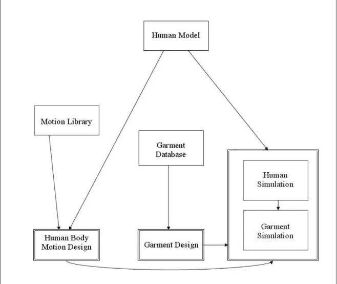
Our system is composed of three modules: motion design, garment design and garment and human simulation. Motion design module allows the user to define various human motion behaviors by adjusting the position, distance and rotation curves of the joint points. The details of this module are out of the scope of this study and they are explained in [35, 61]. Garment design module is an effective tool for creating 3D garments from their 2D panels through cutting and seaming. It enables the designer to position the 3D garment around the virtual character and sew the garment panels. In addition, the system provides different options for rendering garments. Simulation module provides the functionality for human motion, cloth deformation and collision handling. The system architecture is given in Figure 1.1

Figure 1.1: The system architecture

1.3

Organization of the Thesis

The organization of the thesis is as follows: Chapter 2 reviews the state of art in garment design, simulation and rendering fields. Chapter 3 explains the garment design process and Chapter 4 describes the garment simulation process in our system. Chapter 5 overviews the collision handling methods adopted in our sys-tem. Chapter 6 gives some experimental results of the study. Chapter 7 presents the conclusions and future work about the subject. Finally, the system at work and the user interface are explained in the Appendix.

Background

Garment simulation has many potential application areas such as the entertain-ment industry, CAD/CAM systems, e-commerce or textile industry. The evolu-tion of virtual characters in movies, virtual worlds or computer games has created a demand for the dressing of the virtual characters. Hence, the entertainment industry requires fast, convenient and efficient tools for designing garments that look realistic enough. In addition, fashion designers wish to see the appearance of a garment on a virtual mannequin before the garment is manufactured. Similarly, customers of an interactive e-commerce site may opt for trying their garments on and make preferences on the design, texture or color of the garments before they buy them. Thus, CAD/ CAM tools and interactive online stores make use of garment design and simulation systems. Again, these systems require efficiency and realism. On the other hand, textile engineers require accuracy and precision about the behavior of the cloth material. Thus, they deal with the properties of cloth such as Young’s modulus, bending modulus, stress-strain curves, etc. [53]. In the following sections, the state of the art in garment simulation and de-sign will be explained in detail. Garment dede-sign consists of the construction of three dimensional garments from their components, which are cloth panels in 2D. On the other hand, garment simulation deals with the mechanical and geo-metrical modelling, as well as the simulation scheme with numerical integration, environmental interaction and rendering issues.

2.1

State of the Art in Garment Design

Currently, there are various software tools for designing apparel in 2D; however, there is a strong need for 3D tools for designers. Therefore, in recent years, such software has been developed extensively. Garment design using computer graphics has two main approaches:

• designing 2D panels, seaming them and converting them into 3D, and • designing 3D garments around a virtual mannequin and extracting its 2D

components.

The most well-known example for the first type of approach is the MIRA-Cloth Software developed in the Miralab. They find this method more intuitive and similar to real life. In [53], it is stated that the MIRACloth System con-sists of the design of garment patterns, putting patterns on bodies, seaming and constructing garments, animation of garments, defining garment materials and textures, cutting and modifications. In MIRACloth, the design of the patterns consists of editing the garment as a set of 2D polygons linked by seaming lines. Then, these patterns are digitized and triangulated to construct a particle-based system. After that, these patterns are placed around the human body and sewn together. Before the animation, the mechanical parameters of the clothes are set up to reflect the correct behavior of the fabric. Animation is performed by moving the body from a recorded sequence using animation playback. Garments move with the body by means of the reactions to collision response and friction. Similar studies conducted in Miralab include [60, 13, 40].

For instance, the system presented in [60] is one of the initial garment design tools. This is a tool for the interactive design of garments in three dimensions. The system presented for the tool consists of five main parts, which are: the interactive graphic interface for the 2D design of panels, deformable cloth model, pattern library of garment templates, movable human body model and the output interface. The designer draws patterns for 2D garment panels and then these

templates are digitized. It is also possible in the system to animate the garments with human movements.

Furthermore, Protopsaltou et al. present a system for producing 3D clothes with realistic behavior [40]. The main purpose of the system is to build an interactive, compelling and realistic virtual shop, where customers can select the garment designs that they prefer and can see these garments on virtually animated bodies. Using the system, the user can create the standard female or male virtual bodies and create and seem together the 2D garment patterns around the virtual human body. This provides the initial shape of the garment.A simulation is made using the seemed garment by applying physical parameters based on real fabric properties. As a result, the whole system enables the customer to visualize clothes, to animate them, and to add interactivity in addition to view garments fitted onto their own virtual bodies. The main problem in that system is such that the simulation of garment movement is performed using a physics based model, making it impossible to achieve real-time performance. Therefore, the simulation results are prerecorded in order to display the animated garment at an interactive rate.

Later, Cordier et al. present a Web application that provides more powerful manipulation of garment-related items such as sizing and pattern derivation [13]. The customer can select various garments and fit these garments onto the 3D mannequin that is adjusted according to his/her measurements. Moreover, the movement of the garment is simulated to give the customer an idea about how the garment will look on his/her body. The main difference of this system from the one presented in [40] is that the garment simulation is calculated on the fly while keeping the response time interactive. The system sends body/garment sizing as well as cloth/skin animation to the client side. Then, the major part of the content to be manipulated is generated on the client side rather than on the server, which provides a minimal response time to the user. Furthermore, a significant step in this system is the application of 3D graphics technology to create and simulate the virtual store.

The Virtual Try-On project [24] leads the development of new VR technologies that forms the basis of a realistic, three dimensional simulation and visualization of garments put on virtual counterparts of real customers. The complete process chain starts with the 3D scanning of the human body up to a photo-realistic 3D presentation of the virtual customer dressed in the selected pieces of garments.

In addition, the work presented in [11] is a simulator that complements tradi-tional CAD systems that are based on 2D graphics by defining a cross-application data exchange format among the different CAD systems and applications in tex-tile industry. Then, the VRML-based 3D previews of the garment are produced so that they could be published on the Web.

The second type of approach is illustrated in [7]. Bonte et al. outline a 3D graphic environment for industrial applications in the clothing industry in their study. Their system enables the design of a garment in 3D, testing different fabric types on the final garment and the automatic generation of 2D patterns from the 3D representation. 3D modelling of the garment is performed by browsing a library to select the closest garment to the final one and creating the 3D shape by stating values or selecting points or lines on the mannequin. In addition, darts, seams, holes and style lines are defined interactively in the 3D shape. 2D patterns are generated only after the completion of the 3D garment. Flattening is performed by flattening the triangles of the 3D meshes one by one with a non-isometric method and then applying a relaxation procedure to refine the 2D points until error is minimized. In order to simulate the garment in 3D, a particle-based approach is adopted.

The works described in [14] and [15] are also similar to [7] and developed within the framework of the Brite Project MASCOT. In addition, the project “CADwalk” for the 3D display of garments in common PCs is also an example of the second approach [43]. In that study, the figurine can be scaled to the customer’s measurements in order to show the customer how she/he is going to look like in the new clothes. Roediger et al. follow the geometric approach proposed by Hinds and McCartney in [26].

As a final example, Wang et al. present a new approach for intuitively mod-elling a 3D garment around a 3D human model by two-dimensional sketches [55]. First, a feature template for creating a customized 3D garment is defined accord-ing to the features on a human model; second, the profiles of the 3D garment are specified through 2D sketches; finally, a smooth mesh surface interpolating the specified profiles is constructed by a modified variational subdivision scheme. The system has several advantages compared to the earlier approaches. First, the system provides direct design of garment patterns through 2D strokes in the 3D space. In addition, the system enables the regeneration of the patterns when creating the same style of garment for other human models. Furthermore, the 2D sketched input method provided in the system is beneficial for the designers since most designers still prefer to express their creative design ideas through 2D sketches.

2.2

State of the Art in Garment Simulation

Garment simulation includes the geometrical and mechanical behavior of the clothes, interaction of them with the environment and rendering them. In this section, the approaches for the behavior of the cloth model are examined. Then, collision detection and response techniques are reviewed. Finally, rendering tech-niques are presented.

2.2.1

Cloth Model

Before the mid 1980s, cloth was modelled as a texture mapped on rigid surfaces. Today, there are two basic approaches in simulating the cloth using computer graphics: geometrical models and physically-based models. In [8], Breen gives a survey about cloth modelling methods.

2.2.1.1 Geometrical Models

Weil [56] defines a geometric approach that approximates the folds in a con-strained piece of square cloth. He models a cloth hanging from several constraint points. The cloth structure is modelled topologically as a 2D grid of 3D geo-metric points. The first step recursively connects constraint points,with catenary curves as an initial approximation. The grid points lying between the constraint points are placed on the 3D catenary curves. When two curves cross, but do not intersect at the same point, the lower curve is eliminated. New constraint points and catenary curves are then added until all points on the catenary curves lie within the convex hull of the constraint points. The second pass uses a relax-ation technique to enforce distance constraints between all grid points in order to create smooth cloth-like folds in the rectangular grid. Weil does not include any mechanical information in his model. Cloth stiffness is modelled with a second-order distance constraint. He also includes a rendering technique where the cloth surface is subsequently modelled as a collection of cylinders.

Hinds and McCartney [26] present a system for the interactive design of gar-ments by allowing the user to create a geometric model of a garment by specifying the outlines of the garment panels on a mannequin, and then generating offsets from the mannequin surface. They do not physically model the cloth surfaces, instead, folds are sinusoidal offsets added into the geometrical model.

2.2.1.2 Physically-based Models

Physically-based models are more accurate and easier to implement compared to the geometrical methods.

Spring-Mass Models

Haumann and Parent [25] present the spring mass models. Their models in-cluded a point mass, environmental forces, a spring connecting two point masses, a hinge that connects the two triangles formed by two point masses and aero-dynamic drag and wind actors. In this model, each vertex is converted into a

point mass, each edge into a spring and each set of adjacent faces into a hinge. Given initial conditions, the motion of the model is calculated by applying stan-dard Newton’s laws of motion. Their model could not accurately simulate the behavior of woven cloth, only some kind of deformable surface.

Provot [41] describes a similar spring-mass system. The mass particles, ar-ranged in a rectilinear grid are connected with the three types of springs, which were structural, shear and flexion springs. In addition, distance constraints, which eliminate the unacceptable elongations of the cloth are introduced in this method.

Models Based on Elasticity Theory

Feynman [20] simulates some mechanical properties of cloth by defining a set of energy functions over a 2D grid of 3D points. The total energy of this cloth model contains tensile strain, bending and gravity terms. He minimizes the energy of the grid with a stochastic technique and a multigrid method. He assumes that cloth is a continuous flexible material and derived his energy functions from the theory of elastic shells. His energy functions are only based on the distance between points and a simple measure of curvature. His approach does not take into account the shearing behavior of the cloth and the self-intersection of the cloth or interaction of arbitrary solid geometric models.

Taking continuum mechanics and differential geometry as their starting point, Terzopoulos et al. [48] develop a wide range of deformable physically based mod-els. They present a simplified set of equations based on elasticity theory that describe elastic and inelastic deformations, interactions with solid geometry and fracture for flexible curves, surfaces and solids. Their technique for modelling the dynamics of elastic objects uses Lagrange’s equations of motion. The same group also presents works that deal with the practical issues involved in stitching flat panels into three-dimensional clothes and reducing the number and complexity of the model parameters presented to the user.

Baraff and Witkin [5] describe a simple cloth continuum model that is mo-tivated more by numerical computing issues than a desire for mechanical accu-racy. They present a computational framework for producing clothing simulations

based on an implicit numerical integration method. Then, Desbrun et al. [17] ex-tend Baraff and Witkin’s approach to produce real-time simulations of cloth-like sheets which may be interactively manipulated by a user while colliding with or sliding over numerous rigid objects.

Particle Models

Breen and House [9] develop a non-continuum particle model for cloth drape that explicitly represents the micro-mechanical structure of cloth via an inter-acting particle system. Their model is based-on the observation that cloth is best described as a mechanism of interacting mechanical parts rather than a continuous substance, and derives its macro-scale dynamics properties from the micro-mechanical interaction between threads. Crossing points of warp and weft threads are represented by particles. These particles interact with adjacent parti-cles and the environment through mechanical connections represented by energy functions. A stochastic gradient descent technique is used to relax the cloth par-ticles toward a final equilibrium position, producing fabric drape. Afterwards, they showed how this model can be used to produce the drape of specific materi-als accurately. However, the model produces only draped configurations without motion and its original implementation was slow and inefficient [10].

Finite Element Models

Etzmuss et al. [19] present a model based on finite elements that is particularly designed for numerically stiff materials such as textiles. Their system allows fast time stepping by using an implicit integration method. The nonlinear elasticity problem is reduced to a linear, planar one in each step. In contrast to mass-spring models, which deal with regular quadrilateral meshes, this method works independent of the mesh topology.

2.2.2

Integration Methods

During the computation of the evolution of the cloth model, a differential equation system must be solved. Since the cloth system evolves in discrete time steps, the

system should be integrated numerically. There are various integration schemes in the literature. The performance of the integration method depends on the following factors ([54]):

• the computation time for one iteration of the algorithm, • the time step for one iteration,

• the desired accuracy, and • the numerical stability.

Among all the methods, the integration schemes can be classified into two: explicit and implicit methods.

• Explicit integration methods compute the state of the next time step out of

a direct extrapolation of the previous states. Among the explicit integrators, the most important ones are Euler, Midpoint and Runge-Kutta methods. These are relatively easy to implement. However, they need very small integration time steps to guarantee system stability and accuracy.

• Implicit methods deduce the state of the next time step indirectly from an

extrapolation of the next state. These methods are able to use larger steps without loss of stability, but they are more complex to implement because they need to solve large linear systems at every integration step. The use of implicit methods in cloth simulation was first proposed by [5].

The integration methods are explained in Chapter 3 in more detail.

2.2.3

Cloth Rendering

As well as the draping and dynamic deformation of cloth, the visual appearance of cloth is crucial when realism is required. In particular, textiles are mainly divided into knitwear and woven cloth. Therefore, rendering of the cloth can be examined in these two basic types.

2.2.3.1 Knitwear

Meissner and Eberhardt [33] present a system that simulates the real, physically correct appearance of knitted fabrics. They use the produced machine code for knitting machines in their system. For this purpose, they take knitting machine data, generate a data structure representing it and apply a particle system for the physical behavior of the knit pattern. Since their application is almost real-time, they do not integrate time consuming visualization techniques such as ray casting. In order to give the yarn a three dimensional appearance, they use line primitives of different size and brightness. They separate the knitting process into three steps: topology generation, topology reduction and topology refinement. The first step includes the generation of a data structure containing the necessary information of the fabric such as material information, thread course in 3D space and thread interaction points. In addition, this step simulates the operation of a knitting machine. The second step reduces the topology by filtering out all the instable interaction points. Finally, the third step equalizes the distortions by storing the length of the initially distributed thread. To simulate the correct physical behavior, a particle system is adopted. Thus, the dynamics of stretching, repelling and bonding of the yarn are calculated. Spring forces are used to pull or repel the neighboring particles and to simulate the bending of a yarn loop.

Zhong et al. present a method for rendering knitwear on free-form sur-faces [63]. Free-form sursur-faces give the system the potential to consider the in-teraction of the neighboring yarn loops. In addition, the user can determine the fluffiness of the yarn and the irregularity in the yarn positions. In contrast to [33] in which the pattern is based on industrial knitting machines, Zhong et al. model the knitted fabrics made by hand. There are two basic stitches in knitting, plain stitch and the reverse stitch, namely the right loop and the left loop. The knitwear skeleton is composed of an equal partition of a rectangle Q into quadri-lateral tiles based on the stitch pattern, considering the irregularities in the yarn positions. Key points in the parameter domain Q are specified for every loop. Then, these key points are connected by using curve segments to get the loop in 3D. The system is capable of rendering the yarn microstructure efficiently by

drawing free-form knitwear as Gouraud-shaded polygons. The fluffiness of the yarn can be controlled by applying some random perturbations in the positions of the Gouraud-shaded polygons. Although this method is efficient, the results for close-up views are not very realistic.

Another system that uses free-form surfaces is the one presented by Xu et al [59]. In this system, photorealistic rendering of knitwear is handled by introducing an element called the lumislice. The lumislice represents the ra-diance from a yarn cross section. They make use of the fact that the structure of yarn is repetitive and they represent knitwear as a collection of identical lumislices in various positions and orientations. In addition, varying levels of detail for dif-ferent viewing distances is handled by multiresolution lumislices. The framework makes use of hardware aided transparency blending, thus can be implemented easily with standard graphics APIs such as OpenGL. However, this method does not have interactivity.

2.2.3.2 Woven Cloth

When woven cloth is of concern, we cannot simply do texture mapping or ren-dering because occlusion and self-shadowing terms come into scene due to the structure of the individual threads and their interweaving pattern. Similarly, we cannot exactly simulate the real structure as a result of the computational cost. For instance, methods like ray-tracing are costly [16]. In general, methods in this area make use of the periodicity of the weaving or knitting patterns.

Woven cloth is examined in milliscale and microscale. Milliscale geometry refers to how threads are interwoven, whereas microscale geometry is about the structure of fibers making up the yarns.

In [16], the lighting is computed using a geometrical model of a stitch. Then, by sampling the stitch regularly within a plane, a view-dependent texture with per-pixel normals and material properties is generated. The proposed method is interactive since it uses precomputing by keeping a lookup table of the color

and alpha values for each viewing direction. Also, the method is similar to Bidi-rectional Texture Functions and virtual ray-tracing. The base geometry of the knits and weaves are modeled by using implicit surfaces. For rendering, first, a normal is estimated for each visible point on the object. Then, the Bidirectional Reflectance Distribution Function (BRDF) that would be suitable to obtain the color of each pixel is found. After that, the light and the viewing directions are mapped into the geometry’s local coordinate system using the normals. The soft-ware evaluation of the BRDF model returns the three colors and an alpha value from the lookup table, which is then written into the framebuffer.

In [18], the weave of the texture is simulated by procedural displacements of the geometry and the loop is represented as a 2D curve. The 3D appearance is given by displacing the loop. The macroscopic structure of the materials is simulated by using displacement shaders. To model the weave of the material variations, the following function is used.

W eave(x) = cos(2 ∗ π ∗ x ∗ Tf req+ P hase) ∗ Height,

where, Tf req is the number of the threads that is requested, Height is the to-tal amplitude of the weave and P hase is the constant that changes due to the evenness or oddness of the rows.

In order to visualize the close-up appearance of threads, Adabala and Thal-mann present a technique for procedurally creating the texture of the twists of thread in [2]. The tightness of the twist of fibers and the roughness of the fiber are the parameters that have been introduced. The shape of the twist is presented by a trigonometric function. These resulting textures are then combined with color parameters and used to create weave patterns with a realistic look.

Adabala et al. [1, 3] extend their work to generate texture from Weaving Information Files (WIFs), generate micro and macro detail separation and weave based BRDF. The BRDF is generated by the WIF information.

2.2.4

Collision Handling

Garments interact with the body or with other garment panels. The shape and the movement of the body affect the garments movement. Thus, in order to obtain realistic simulation of garment panels, collision handling must be achieved in an accurate and efficient way.

Collision handling consists of two phases:

• Collision detection: Checking the geometrical contacts and proximities

be-tween the objects.

• Collision response: Correcting the velocities and positions of the colliding

objects by applying constraints or forces.

2.2.4.1 Collision Detection

Collision detection is the most time consuming part of the cloth simulation, since the number of geometrical entities, such as nodes, faces, and edges that the collision detection algorithm has to handle is large. The complexity problem leads the development of algorithms that decrease the number of collision tests. Most of these algorithms make specific assumptions about the objects and design solutions based on the geometry of the objects. Lin and Gottschalk [31] have presented an overview of collision detection methods.

The general case of collision detection is the one involving cloth and an object. A particular case is the self-collision detection or the collision between a garment panel and the human body.

Collision Detection Between Cloth and Human Body

Collision detection between cloth and the human body has been widely stud-ied in the last decade. Most of these methods use geometrical collision detec-tion methods with the optimizadetec-tion techniques in order to reduce the number of checks.

Mezger et al. [37] propose a method by combining and improving the tech-niques, such as hierarchical bounding volumes [51], collision prediction (proxim-ities) through k-DOPs bounding volumes [30] and heuristics [51]. They improve the efficiency of bounding volume hierarchies by adapted techniques. To prune the hierarchy, extended sets of heuristics, such as curvature and coherence crite-ria, are used. In addition, for preserving large time steps and stability, oriented inflation of bounding volumes is used to detect not only collisions but also prox-imities. The advantage of this approach is to detect collisions before they occur. A voxel-based collision detection method for clothed human animation is pre-sented in [62]. They speed up the performance of the voxel-based method by choosing an appropriate voxel size and using a fast voxelization approach. Based on the voxel method, they propose a self-collision detection method and a sim-plified collision detection method. Firstly, the efficiency of self-collision detection is improved by taking advantages of the curvature and multi-layer methods. Sec-ondly, the efficiency of cloth/human collision detection is improved by introducing auxiliary line segments. Experimental results demonstrate that their method is efficient for clothed human animation. It has, however, a limit in that it can’t be applied to interactive garment simulation in the aspect of speed, and it is hard to apply to fast movement since it can only handle collisions occurred in the current frame.

Vassilev and Spanlang [49] propose a cloth-body hardware-assisted method that uses z-buffer not only to compute the depth maps of the body but also to interpolate the body normal vectors and velocities of each vertex. Although the method is fast and does not depend on the complexity of the human body, the maps need to be precomputed for each simulation, which makes it difficult to use in the applications

In addition to the above methods, approaches for animating dressed humans are proposed based on the property that most parts of a garment do not change position relative to the human body [12, 44]. The system described in [12] per-forms real-time animation of complex garments by classifying the particles of the garments into layers and applying different animation techniques for each of

them. The deformation and collision handling of the layers are done depending on how they lie on the body surface and whether they stick or flow on it. The cloth layers are categorized as: stretch, loose and floating clothes. The results in [12] show that the method achieves real time performance compared to the other cloth simulation approaches. In addition, this method can be used only on top of deformable objects such as virtual humans since it uses the deformation of the underlying object.

Self Collision Detection

Self-collision detection is a special case of collision detection where both of the intersecting geometrical primitives belong to the same deformable model. It is a complex task compared to the collision between cloth and an object because some special cases, such as multiple collisions, collision consistency and adjacency in bounding boxes, should be examined carefully. Several methods have been proposed for handling self-collisions accurately and efficiently.

Particular advances in accelerating the self-collision detection are achieved by Volino et al. [51]. They propose a method that is based on geometrical shape regularities. They used a region-merge algorithm to build hierarchies on top of a polygonal mesh, storing adjacency information for the regions. In order to avoid unnecessary self-collision tests in whole branches of the tree, they use the surface curvature optimization method. This method is based on the property that, when a given zone has sufficiently ”low curvature”, it cannot self-intersect, and all the zones it includes do not intersect with each other. This means, if the branches of the tree correspond to a zone with a sufficiently low curvature, no self-intersection test is done. Furthermore, they also introduce a technique that observes the history of close regions to guarantee a consistent collision response [50]. In their recent publications, they use the k-DOPs as bounding volumes [52].

Provot [42] uses the bounding box hierarchy and surface curvature method [51] for optimizing collision detection. He creates the bounding box hierarchy of the tree by recursively dividing the cloth piece into zones considering the triangles positions. Then, the curvature information of each node is updated bottom-up by using the two angles of its descendant nodes, α1 and α2. The leaf nodes have

angle α = 0, since they have single normals. In self-collision detection, while parsing the tree, the algorithm eliminates the nodes whose bounding boxes do not intersect. In addition, the surface curvature is also considered. If the angle

α > Π, then self collision detection is applied. Otherwise, it is not.

Huh et al. propose one of the best solutions to self-collision problem [27]. They consider the cloth-cloth collision resolution as a special case of deformable N-body collision resolution. They group the particles into parts and using the law of momentum conservation they handle the collisions between these parts. They create a system of linear equations for resolving collisions using a scheme adapted from the simultaneous resolution method for rigid N-body animation. The linear equations are built from the collision relations for the cyclic relatioships in collisions.

Despite some speedup techniques, such as curvature of the cloth surface [52, 42] and bounding volume hierarchies, self-collision handling often fails to get real-time performance.

Optimizing Collision Detection

Optimization techniques are used for efficient collision detection by preventing

O(n2_{) comparisons. There exist many algorithms depending on the complexity}

reduction mechanism behind them [53]. The main groups are:

• Bounding Volumes: Complex objects or object groups are enclosed within

simpler volumes, such as box, sphere, that can be easily tested for collisions.

• Projection Methods: Possible collisions are estimated by using separately

the projections of the scene along several axes or surfaces.

• Subdivision Methods: The problem is decomposed into smaller space

vol-umes or object regions either on the scene space or on the object space. They are usually evaluated through bounding volume techniques. Hierar-chical subdivision schemes add efficiency.

• Proximity Methods: The scene objects are arranged according to their

ge-ometrical neighborhood. The collisions between these objects are detected based on the neighborhood structure.

2.2.4.2 Collision Response

Once the collisions have been detected for a given frame, their effects, such as preventing objects from interpenetrating, and producing contact reaction, have to be taken into account in the mechanical simulation. Collisions between de-formable objects are much more difficult to treat than collisions between rigid objects, because a response for each face or particle has to be computed and care must be taken not to introduce additional stiffness.

Several collision response schemes for cloth animation have been presented. In general, there exist four options for the collision response:

• Constraint-based: This approach assumes totally inelastic collision. The

particle that has collided with an object is constrained to lie on the surface of the object. The collision response is integrated as a direct correction on the state of the system. This approach is presented by Baraff and Witkin [5]. Later, Volino et al. [52] have used the approach that is based on correction of positions, velocities, and accelerations of colliding particles.

• Penalty-forces: In this method, a spring force that keeps particles away

from each other is applied.

• Impulse-based: This method applies an “instantaneous” change in

momen-tum. The main advantage of this method is it correctly stops all collisions. However, it can have poor numerical performance and it handles persistent contact poorly.

• Rigid body dynamics: The basic idea behind this option is if a group of

particles start time step collision-free, and move as a rigid body throughout the time step, then they will end time step collision free. For applying this

idea to the cloth, we can group particles involved in a collision together and move them as a rigid body. This method is totally failsafe. Until the impact zone includes all colliding particles, we will need to iterate, and merge impact zones. This method is proposed in [42] and it is used as a last resort. Although it is easy to implement, when the particles collide into each other it cannot get dynamic interactions between particles.

The Garment Design

3.1

The Cloth Model

The cloth model used in our system is a mass-spring model [41], which behaves according to the Newton’s second law of motion F = ma. This is a specific case of a particle system, in which the particles are connected by spring forces. Particles are objects that have mass, position, and velocity, and respond to forces, but that have no spatial extent. The type and behavior of the cloth is determined by the strength of the spring forces and the topology of the cloth, which is determined by how the springs connect the particles. The mass-spring model is adopted due to its simplicity, efficiency and the capability to simulate the physical behavior of cloth.

The cloth system is simulated by calculating the positions of each particle, which depend on the forces acting on each particle. These forces can be divided into two as the internal and external forces. Internal forces are the spring forces, whereas external forces are the forces such as gravity or wind.

The initial grid structure is a rectangular mesh of particles at the vertices and the springs connecting these particles (Figure 3.1).

3.1.1

Internal Forces

Internal forces are the spring forces between the particles and they determine the mechanical properties of the cloth. These mechanical properties can be catego-rized into four as follows ([53]):

• Elasticity: Characterizes the internal forces resulting from a given

geomet-rical deformation.

• Viscosity: The internal forces resulting from a given deformation speed. • Plasticity: Describes how the properties evolve according to the deformation

history.

• Resilience: Defines the limit at which the structure will break.

3.1.1.1 Springs

A spring, whose behavior depends on the Hooke’s law, is defined by the tension between the endpoints of that spring. The forces on the endpoints of the spring (fi and fj) depend on the rest length (rij), the spring coefficient (ks), the damping constant (kd), the velocities of the endpoints (vi and vj) and the current length of the spring (dij).

fi = −[ks(|dij| − rij) + kd(vi− vj)( dij |dij| )]( dij |dij| ) dij = posi− posj fj = −fi

The spring force magnitude is proportional to the difference between the ac-tual length and the rest length, while the damping force magnitude is proportional

to Pi and Pj’s speed of approach. Equal and opposite forces act on each particle, along the line that joins them.

Three types of springs are used in order to reproduce the stretching, shearing and bending behavior of cloth.

1. Structural springs: These springs connect the vertices adjacent along the row or column of the grid. Namely, they connect the particle [i, j] with particles [i+1, j] and [i, j+1]. The cloth is made up of warp and weft fibers and these springs model this fact. Structural springs serve to keep the cloth in its natural rectangular state.

2. Shear springs: They connect the two vertices along the diagonals of each rectangle in the mesh. Namely, they connect the particle [i, j] with particle [i+1, j+1] and the particle [i+1, j] with particle [i, j+1]. The shear springs prevent the cloth from collapsing. They handle the shear stress of cloth. 3. Bend springs: These springs connect every other particle along the two

directions of the rectangular grid. Namely, they connect the particle [i, j] with particles [i+2, j] and [i, j+2]. These springs prevent the cloth from bending excessively. Keeping these springs stiff restricts the cloth from bending too much out of the original plane of the grid.

Instead of adding shear springs, the realistic behavior of cloth can also be simulated by increasing the resolution of the grid. However, this brings a high computational cost to the system; thus, the realism is achieved by adding shear springs.

3.1.2

External Forces

The external forces that have been implemented in our system are gravity, viscous drag, wind and collision forces. The first three are presented in this section, whereas collision forces are described in Chapter 5.

Figure 3.1: Cloth mesh with springs and masses

3.1.2.1 Gravity

The global earth gravity acting on each particle is f = mg, where g is a constant vector whose magnitude is the gravitational constant. The gravitational force is applied simply by traversing the system’s particles, adding the appropriate force into each particle’s total forces.

3.1.2.2 Viscous Drag

The effect of drag is to resist motion, making a particle gradually come to rest in the absence of other influences. In order to enhance numerical stability, at least a small amount of drag should be applied to each particle. Ideal viscous drag has the form f = kdv, where the constant kd is called the “drag coefficient” [58].

3.1.2.3 Wind

A nonlinear wind formulation in accordance with fluid laws in physics is used in our system.The force acting on a triangle due to wind is always in the direction of the normal vector of that triangle. The force is proportional to the surface

area of the triangle, the angle at which the wind hits the triangle, and the speed of the wind.

Each mass point having approximately the same small surface area, we assign a drag force due to wind to a mass point Pi as:

F_idrag = kdkvwindi k(ni· viwind)ni,

where vwind

i is the velocity of the wind, ni is the surface normal and kd is a dragging constant. First, the drag forces are calculated for each triangle. Then, the total drag force for each point is calculated as the sum of the drag forces of the triangles surrounding that point [36].

3.1.3

Evolving the Cloth in Time

In order to compute the progression of the system in time, the system must be integrated numerically. The progression is calculated as a sequence of successive positions of the particles making up the cloth, over specific time intervals. The integration methods can be basically classified into two: explicit and implicit methods [58].

We have implemented both implicit and explicit integrators in our system so that the best one could be selected depending on the circumstances.

3.1.3.1 Explicit Integrators

Euler Integrator : This method is the simplest method for numerical integration.

The formula for this method is

x(t0+ h) = x0+ hx0(t0)

In this way, instead of calculating the true integral of the function f in x, we find the approximate solution by taking a step size of h in the direction of the derivative. However, the derivative information is used only at the beginning of the interval.

We can adapt this formula into our system as:

x(t0+ h) = x0+ hv(t0)

Where, v is the initial velocity of the particle, x0 is the initial position of the

particle and x is the position of the particle at time t0+ h.

By applying a Taylor series expansion, we can see that the error in Euler integrator is O(h2_{) [39].}

Midpoint Integrator : Euler Integrator may go unstable if large step sizes are

taken. From the Taylor series, if we knew the second derivative of x, we could get an error of O(h3_{). Thus, we take a trial step to the middle of the interval and}

then use the value of the x and x’ at the middle of the interval to calculate the real step across the interval. We obtain:

x(t0 + h) = x0+ h(f (x0+h

2f (x0))

Runge-Kutta Integrator : The same idea can be further improved for less error

rates. We take several Euler steps and in each step, the derivative is evaluated four times: once at the initial point, twice at the midpoints, once at a trial end point. Then, the final function value is calculated as:

k1 = hf (x0, t0) k2 = hf (x0+ k1 2, t0+ h 2) k3 = hf (x0+ k2 2, t0+ h 2) k4 = hf (x0+ k3, t0+ h) x(t0+ h) = x0 + 1 6k1+ 1 3k2+ 1 3k3+ 1 6k4 In the fourth order Runge-Kutta, the error term is O(h5_).

Adaptive Runge-Kutta: Runge-Kutta integrator can be improved by applying

adaptive step size. The purpose is to achieve accuracy in the solution with mini-mum computational effort [58]. In implementing adaptive integrators, we get two stepsizes, calculate the error and increase or decrease the stepsize depending on the error threshold.

3.1.3.2 Implicit Integrators

Even the higher order explicit methods require small time steps in order to pre-serve stability. However, since implicit integration methods consider information of the next time-step, large stepsizes can be taken in order to deduce the next state. In [5], Baraff and Witkin proposed to use implicit integration so that the cloth simulation with stiff equations could be possible. The results presented by Baraff and Witkin showed that, implicit integration methods allowed to take large time steps so that the efficiency of the system would not be reduced.

Implicit Euler Integrator : The method in [5] requires the solution of a linear

system with O(n2_{) computation time, where n is the number of mass points in}

the cloth. In our study, we have followed the approach presented in [28] in order to implement implicit integration. This method enables the simulation of the system interactively.

x(t + h) = x(t) + hv(t + h) (3.1)

which is different from explicit integrators since they consider the value of the velocity at time t. However, implicit Euler requires that we know the value of

v(t + h). This value is:

v(t + h) = v(t) + hM−1_{f (t + h) (3.2)}

where,

f (t + h) = f (t) + ∂f

∂x∆x(t + h) = f (t) + Jx(t + h) (3.3)

So, from (3.1) and (3.3) we get:

x(t + h) = f (t) + Jx(t + h) = f (t) + J(v(t) + v(t + h))h (3.4)

where,

∆v(t + h) = hM−1_{f (t + h) (3.5)}

= hM−1_{f (t) + h}2_M−1_{Jv(t) + h}2_M−1_{J∆v(t + h) (3.6)}

By rearranging Equation (3.6), we finally obtain:

(M − h2J)v(t + h) = hf (t) + h2Jv(t) (3.7)

The solution of (3.7) returns us the value of v at time t + h.

The algorithm exploits the fact that the matrix (M − h2_{J) is sparse and}

symmetric. In this way, applying iterative methods solves the problem in real time.

3.2

The Garment Design Process

The garment design process consists of the following phases: First, cloth meshes, each a rectangular grid of vertices, are created. Then, the garment panel is given its desired shape via cutting or selecting individual vertices and moving them or automatically smoothing the boundary. After creating the flat panels, seaming points can be defined on them. This is done by selecting the vertices to attach and adding seams between them. In addition, the obtained garment panels can be scaled to the desired size.

3.2.1

Creating Garment Panels

A garment panel is a rectangular grid showing the positions of particles and springs. While creating these panels, the user can specify the number of parti-cles in the mesh, spring constants for bend, shear and structural springs (which determine the type of the fabric material) and the size of the cloth mesh.

3.2.2

Cutting

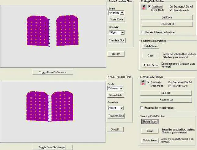
There are two options for cutting fabric in order to design garments: either to draw the 2D shape of the garment and then discretize it, or to select the cloth boundary on an already discretized cloth mesh. The latter is more similar to the cutting process in real life and it also preserves the regular structure of cloth. In our system, we prefer the second option since we need regularity for rendering knitted and woven fabric. We select the particles that make up the cloth boundary and then cut it out of the rectangular mesh (Figure 3.2).

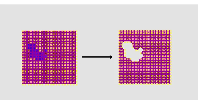
When applying cutting, we perform the 8-connected, recursive boundary fill algorithm on the particles making up the cloth mesh, thus by only selecting the boundary of the cloth it is possible to extract the desired pattern. There are also other options such as extracting out pieces and creating holes on the cloth piece as in Figure 3.3.

Figure 3.2: The 2D garment panel cutting process

3.2.3

Smoothing

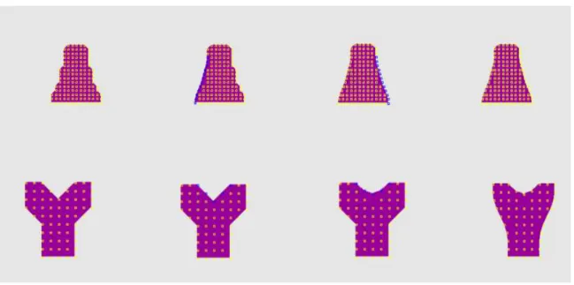
After the cutting, we can smooth the boundary of the cloth panels with the intention of preventing the jagged borders. In order to apply smoothing, we select the particles on the boundary that require smoothing as control points, and then calculate the B´ezier spline for these control points and move the particles onto the resulting curve. B´ezier curves are preferred over other spline approximation methods since they are easy to implement and powerful for designing curves [6]. Figure 3.4 shows the smoothing process on a skirt and shirt.

The B´ezier spline approximation is performed on a set of n + 1 control point positions: pk = (xk, yk, zk), where k ∈ [0, 1, 2, ..n]. These control points can be blended to vector P (u), to describe the path of an approximating B´ezier polynomial function between p0 and pn.

P (u) =

n

X

k=0

pkBEZk,n(u), 0 ≤ u ≤ 1

where BEZk,n(u) are the “Bernstein polynomials”:

BEZk,n(u) = C(n, k)uk(1 − u)n−k

and C(n,k) are the binomial coefficients:

C(n, k) = n! k!(n − k)!

3.2.4

Seaming

Seaming is performed by defining the seam points between the particles of cloth panels. The process can be seen in Figure 3.5.

Figure 3.4: Smoothing the boundary of 2D garment panels

Another option is to perform “batch seaming”, that is, instead of defining the seam points one by one, selecting the line of seaming on one cloth piece and then bringing the two cloth pieces close enough and seaming the points all at once. This method works by finding the closest pair of particles between the two clothes and adding seams between them. Figure 3.6 shows this process.

3.2.5

Resizing

In order to fit the garment on the mannequin, it should be resized taking the sizes of the mannequin into consideration. This process is performed through scaling the panel as a whole or selecting certain particles and translating them individually.

Figure 3.5: Seaming 2D garment panels

The Garment Simulation

The garment panels are transformed from 2D to 3D in order to simulate the three dimensional behavior of garments. Then, the panels are placed around the virtual human and sewn together. The user can modify the rendering options and determine how the garment is going to look like at the end so that he/she can see the final appearance of the garment.

This chapter examines the garment simulation process implemented in the scope of this thesis study.

4.1

Garment Placement

Garment panels are placed around the body by keyboard interaction. It is possible to translate, scale or rotate each garment panel. In addition, local parts of a garment panel can be translated individually. This is achieved by changing the position of the selected particles. In this way, the garment panel can obtain the desired shape.

4.2

Sewing

After garment panels are in their accurate positions around the body, sewing is invoked by applying forces between the seams in garment parts. Seams can be regarded as forces that attract two particles to each other (Figure 4.1), in that sense, they can be regarded as elastic forces. However, simulating the exact be-havior of elastic forces is expensive [53] and a much simpler heuristic can solve the problem more efficiently. The heuristic approach is applying symmetrical forces on the two particles so that they pull each other as in the following equations:

p1vel = cattraction

|p1pos− p2pos|

kp1pos− p2posk

p2vel = −p1vel

Figure 4.1: Forces acting on particles during the sewing process

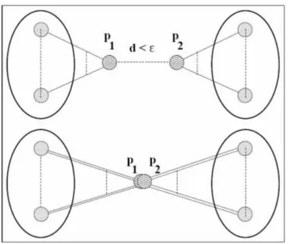
The two particles attract each other until they are constrained by collision forces. During the sewing process, no other forces such as gravity are applied on the clothes. After two particles p1 and p2 are closer than a threshold, the

sewing process is finalized and these particles are combined into one. This is performed by adding spring forces between p2 and neighbors of p1 and between

p2 and neighbors of p1 (Figure 4.2). Neighbor of a particle p means the particle

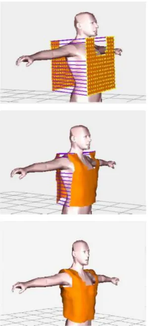
q such that there exists a spring between p and q. In Figure 4.8, the procedure for placing parts of a shirt and sewing them can be seen. By this approach, the garment can be a complex assembly of different textile materials.

Figure 4.2: Combining two particles into one after sewing

4.3

Attachment Constraints

In order to keep the garment on the virtual model without losing efficiency, some parts of the clothes can be attached to the human body. This approach is followed depending on the type of the garment. For instance, tight clothes can be bound to the human body with attachment constraints. For this purpose, after the virtual human is dressed with the garment, the selected particles are attached to the closest polygon on the virtual human. In this way, those parts of the garment move with the human.

4.4

Rendering Garments

Realistic rendering of clothes is as important as the simulation of their draping since important information about the material the fabric is made of can be ob-tained via its visual appearance. Besides general rendering techniques such as

Gouraud shading, some shading techniques specifically related to textiles exist. There are various methods to produce garments from yarn, such as knitting, weaving, braiding or knotting. The most important ones among these are knit-ting and weaving. Thus, we have simulated these two methods in our system. Moreover, standard methods and material-specific BRDFs are also implemented. This section explains the techniques that have been implemented for rendering garments.

4.4.1

Smoothing

Before explaining the methods for weaving and knitting, we should make sure that the surface is smooth enough. In order to have a smooth surface, we rediscretize the surface by taking into account surface geometry. Thus, flat mesh triangles are converted into curved surfaces, which give the cloth a smoother appearance. This method is adopted from [53]. The procedure is very simple since it considers only vector positions and vector normals for each triangle. The discretization scheme is as follows:

Given Pa, Pb, Pc vertex positions and Na, Nb, Nc vertex normals, let P = (raPa, rbPb, rcPc) be an intermediate point on the triangle where ra, rb and rc are barycentric coordinates and N = (raNa, rbNb, rcNc) is the normal of point P. Our aim is to calculate an interpolated point Q. For this purpose, we calculate the contributing points Qa, Qb and Qc that make up Q (Figures 4.3 and 4.4).

Ka = P + ((Pa− P ) · N)N

Qa = Ka+

(Pa− Ka) · Na 2 + µ((N · Na) − 1)

Q = f (ra)Qa+ f (rb)Qb+ f (rc)Qc f (ra) + f (rb) + f (rc) where, f (x) = x2

Figure 4.3: Contribution of the vertex Pa to the smoothed vertex P during the smoothing process (reprinted from [53])

Figure 4.4: Interpolation between vertex contributions during the smoothing pro-cess (reprinted from [53])

4.4.2

Knitwear

The structure of knitwear is complicated compared to other techniques like weav-ing. This is due to the three dimensional geometry of a knit loop. In our system,

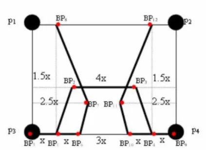
we make use of the particle system and the mass-spring model of our cloth mesh in order to consider the interaction of neighboring loops. For this purpose, the cloth mesh must consist of quadrilaterals and must be regular. There are two types of basic stitches when knitting: left and right loops. The knitwear pattern, which shows the order of the right and left loops is read from an input file and can be changed interactively in the program.

Each quadrilateral contains one type of loop. The structure of the loop in a quadrilateral is defined by the bonding points (BPs). The position of the bonding points can be determined parametrically by the vertices of the enclosing quadrilateral. The equations obtained from the parametrization of the surface are as follows: BP1 = 6 7p3pos+ 1 7p4pos BP2 = 5.5 21p1pos+ 1.5 21p2pos+ 11 21p3pos+ 3 21p4pos BP3 = 1.5 21p1pos+ 5.5 21p2pos+ 3 21p3pos+ 11 21p4pos BP4 = 1 7p3pos+ 6 7p4pos BP5 = p3pos BP6 = 5 7p3pos+ 2 7p4pos BP7 = 4.5 28p1pos+ 2.5 28p2pos+ 13.5 28 p3pos+ 7.5 28p4pos BP8 = 6 7p1pos+ 1 7p2pos BP9 = p4pos BP10 = 2 7p3pos+ 5 7p4pos BP11 = 2.5 28p1pos+ 4.5 28p2pos+ 7.5 28p3pos+ 13.5 28 p4pos BP12 = 1 7p1pos+ 6 7p2pos

of vertices.

Due to the thickness of the yarn, these bonding points are moved slightly taking the normal of that quadrilateral into consideration. Then, each bonding point Bpiis assigned the value Bpi+N, where N is the surface normal. Thus, the knitted fabric looks different when front and back views are considered. Figure 4.5 shows the construction of the loops.

In order to maintain interactivity, complex volumetric models or time con-suming methods like the ones in [59, 34] for rendering the yarns in a loop cannot be utilized. 3D effect for each yarn is achieved by drawing cylinders around each yarn and applying texture mapping on these cylinders. However, since this operation also slows down the system, except for close-up views, we draw line primitives of different sizes and colors so as to give a three dimensional look, similar to Meissner et al. [33]. Figure 4.9 shows the close-up view of a knitwear.

4.4.3

Weaving

The woven cloth effect cannot be captured realistically by texture mapping; a cloth simulation program should enable the user to create complex patterns and determine the material of the fabric interactively. At this point, procedural sim-ulation techniques of the visualization of cloth can be adopted. For representing the behavior of woven fabric, the interweaving of threads and the interaction of the light with threads should be carefully integrated. Weaving should be exam-ined in two scales: milliscale and microscale. Milliscale examination refers to the order of the interleaving of threads, whereas microscale examination deals with the fibers constituting the threads [57, 1].

4.4.3.1 Representation of Interwoven Threads

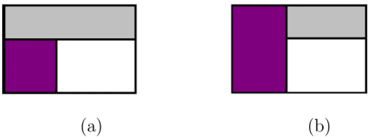
In actual life, weaving can be performed by means of a loom. The idea of the loom is to interleave two sets of perpendicular threads [21, 22, 23]. These threads are the warp and the weft threads as can be seen in Figure 4.6. Warp threads are the vertical ones, whereas the weft threads are the horizontal ones. Weaving patterns can be obtained from two types of interleaving of threads, i.e. warp on weft and weft on warp.

(a) (b)

Figure 4.6: Obtaining weave patterns by interleaving threads. (a) weft on warp; (b) warp on weft.

Various weaving patterns can be created by ordering these two thread inter-leaving types. Our system works as follows: we read the patterns from a pattern