A heuristic procedure for a single-item dynamic lot sizing problem

Computers ind. Engng Vol. 14, No. 2, pp. 181-192, 1988 0360-8352/88 $3.00+0.00

Printed in Great Britain Pergamon Press plc

A H E U R I S T I C P R O C E D U R E F O R A S I N G L E - I T E M D Y N A M I C L O T S I Z I N G P R O B L E M

O . S. BENLI, l I. SABUNCUOGLU 2 a n d S. TUFEKCI 3

IDepartment of Industrial Engineering, Bilkent University, 2Department of Industrial Enginering, Middle East Technical University, Ankara, Turkey and 3Department of Industrial and Systems Engineering,

University of Florida, Gainesville, Florida, U.S.A.

(Received for publication 24 April 1987)

Abstract--An O(T) heuristic procedure for a single-item dynamic lot sizing problem is intro- duced in this paper. The algorithm tries to establish the regeneration points of the problem whether either the production or the beginning inventory must be equal to zero. The proposed algorithm is very easy to implement and compares very favourably with the existing heuristic procedures.

1. INTRODUCTION

Single-item dynamic lot sizing (SIDLS) problems have been the focus of numerous researchers in recent years [1-24]. This is due partly to their importance as production planning tools in materials requirements planning as well as being a crucial part in the development of multi-item production planning models.

The SIDLS problem can be expressed as follows: for each period t = 1, 2 , . . . , T, let D, be the known demand, Xt be the number of units produced, Ft be the on hand inventory, and I t be the units backordered at the end of the period. Also let ft(Xt), h~+(l+), h7(17) be the cost functions associated with production, inventory, and back- ordering at period t, respectively. The objective is to determine a production schedule X = (Xt,)(2, • . . , Xr) that minimizes the total production, inventory, and backordering costs over T periods while satisfying all demands.

As an optimization problem SIDLS can be formulated as follows:

minimize f( X , l ÷, I - ) =

T

E [f,(X,) + h,+(l, ÷) + h,-(l,-)] (1)

t = l

subject to X, + 1, +_ ~ - 1, + + I,- - I,_Z1 = D,, t = 1,2 . . . T (2)

I o-=1o + = I ~ = I r = 0

(3)

X,,It+,It->~O, t = 1 , 2 . . . . T (4)

When h7 and h7 are linear and ft is piecewise linear convex for all t, then the corresponding SIDLS problem may be cast into a transportation problem [1-5]. Several greedy algorithms have been developed for this variation of the SIDLS problem. Johnson [4] treated the problem with no backorders allowed. Posner and Szwarc [5] treated the problem with backorders where holding and backorder costs are assumed to be constant over time. Erenguc and Tufekci [3] treated the problem with time varying costs. All these algorithms are based on transportation formulation of the SIDLS problem.

For the case where the system costs are convex, Veinott [6] formulated the SIDLS problem as a convex cost network flow problem. The optimum solution can be obtained by satisfying each unit of demand through the current cheapest route in this network.

When the cost functions are concave the SIDLS problem becomes an NP-hard problem. Wagner and Whitin [7] formulated the problem as a dynamic programming problem. Numerous extensions of the concave cost SIDLS problem have been analyzed

182 O.S. BENLI et aL

by a number of researchers [8-10] since the seminal paper of Wagner and Whitin. Many of these algorithms require a considerable knowledge of optimization, branch-and- bound procedures and integer programming.

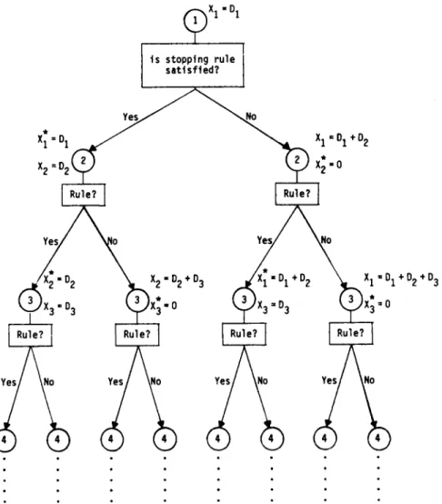
The desire to obtain reasonably good solutions in a very short time period, without indulging into optimization techniques, have led to the development of numerous heuristic procedures. Among the most prevailing ones, we can list Gaither [11], Silver- Meal [12], Groff [13], Part Period Balancing [14], Least Unit Cost [15], Periodic Order Quantity and Economic Order Quantity [16]. All these heuristics are one pass pro- cedures on the SIDLS problems with constant production, setup and inventory costs with no backorders. Some have look-ahead and/or look-back features. They all start with a current period and accumulate the demands of succeeding periods to be satisfied with the planned production in the current period until a prescribed rule is met. This procedure is then repeated for the remaining periods whose demands are not yet satisfied. A general scheme of these heuristics is presented in Fig. 1.

X 1 = D I X 2 = O 2

~

X 1 - D I is stopping rule s a t i s f i e d ?

X 1 = O 1 + D 2

X~ -0

Ye.~

~1o

k ~ 1 3

Ye/

/12 "D 2 12 - D 2+ D 3 -D I +D 2

X 1 =DI+D2÷D3

'X*~ =0

Yes/ ~No

Fig. 1. A general scheme for lot-sizing heuristics.

f

It is shown by Axsater [17] that the solution obtained by Silver-Meal heuristic can be arbitrarily bad for sharply decreasing demand patterns. That is, the ratio of the cost of the solution from this algorithm to the ratio of the optimal solution can be arbitrarily large. Axsater also showed that the same ratio for Part Period Balancing heuristic can never exceed 2. Another demand pattern which causes poor performance in Silver-Meal

A heuristic procedure for a single-item dynamic lot sizing problem 183 heuristic is a pattern with frequent zeroes which is quite common in materials require- ment planning. To overcome these shortcomings Silver and Miltenburg [18] have pro- posed a modified heuristic. However the proposed heuristic is no longer a one-pass algorithm. It is more complicated and requires additional computational time.

Gaither's original algorithm [11] performs quite well for problems with low ordering costs and high carrying costs. However, as indicated by Silver [19] the algorithm degenerates quickly as the ratio of ordering cost to carrying cost increases. To overcome this problem Gaither [20] proposed a "correction factor" for the carrying cost. This factor considers the coefficient of variation of the demand data and the ratio of ordering cost to carrying cost. This new modified algorithm is compared favorably to Silver-Meal [12] and Groff [13] algorithms.

In this paper we propose a new one-pass heuristic for the SIDLS problem treated by all the heuristics presented above. In Section 2 we present this heuristic. The comparison of the proposed heuristic to other heuristics is presented in Section 3. Section 4 concludes our work.

2. DEVELOPMENT OF THE PROPOSED HEURISTIC

The SIDLS problem considered in this paper and all other heuristics has the following functions, for t = 1, 2 . . . T:

ht_(lt_)= { ofOr I t-

> 0 f o r / , - = 0 ' h,+ (It ÷)

=hlt÷,for lt + >10,

(5)

K if X t > 0 (6) f,(X,) : if X, = 0

Note that since the unit production cost is assumed to be constant for all periods and since the total demand must be met, the total variable cost of production is constant for the planning horizon. Therefore, ft reflects only the setup costs. Moreover, the model assumes backordering is not allowed.

In the case of concave costs, one of the most important properties of the SIDLS problem, as stated in [7], is that there exists an optimal solution such that, at any period, either the production or the beginning inventory must be equal to zero. In literature [21], a period t is called a regeneration point if It-~ "X~t = 0. This implies that if a production takes place in a given period, the amount of production (or the lot size) must equal the sum of the demands for an integral number of periods.

If these regeneration points can be identified, then the corresponding lot sizes can easily be determined by simply summing the demand between the regeneration points.

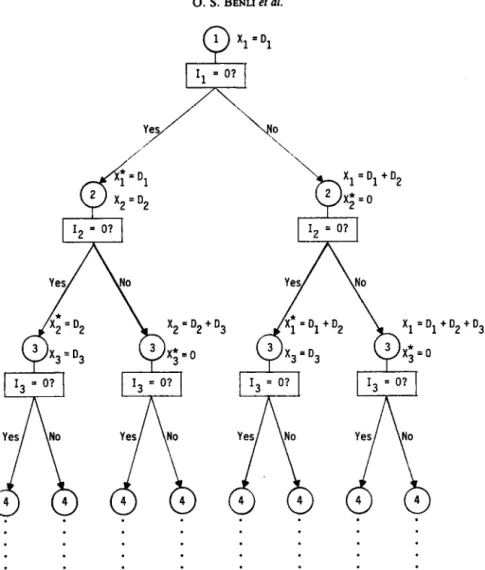
The proposed heuristic starts from the first period with non-zero demand. It scans each successive period by adding that period's demand to the current lot-size until next regeneration point is reached. Once such regeneration point is established, the same procedure is repeated for the remaining periods. Let j t> 1 be the earliest period with non-zero demands. The algorithm sets t = j and X~/ =

Dr.

It then considers whether period t+ 1 is a regeneration point or not. This is accomplished by a rule to be established in the next section. If the answer is "yes" then j is set to t+ 1 and

t=j

and the argument starts anew. If the answer is "no" then

Dt+t

is added to X; and t is increased by 1. The question of whether t+ 1 is a regeneration point or not is asked again and the argument continues until the last period is considered. A general scheme of the proposed heuristic is presented in Fig. 2.

In what follows we will develop the necessary criteria for testing if, for a given scheduled production in period j, and the demands of periods j to t, t ~> j already

184 0. S. BENLI er al. . . . . . . . . . . . . . . . . I3 = 01

a

Yes No 4 4 . . . . . . . . . . D2 +D2+D3 I3 = D? Yes No

n

4 4 . . . . . . . . . .

Fig. 2. Schematic procedure of the proposed heuristic.

committed to this production, if period t+l is a regeneration point or not. Since at any time three successive periods t, t+l, and t+2 will be considered, this will be called a 3- period criteria.

j-Period criteria

Suppose the last scheduled production is in period j, and the demands of periodsj to I, c 2 j already committed to this production. Concerning periods t+ 1 and t+2 we have four possible states based on whether they are regeneration points or not.

Knowing the last production point j, and the states of periods t+l and t+2, we can determine the incremental cost to be incurred if any of these four states is accepted. Table 1 below presents these four states and their incremental cost contributions to the total cost function. The algorithm accepts the state Si for which

C(S,) = minimum { C(SJ} for j = 1,2, 3,4.

Once the state of period t+ 1 is determined the process starts anew in period t+ 1. Let M = K/h. For the period t+l to be a regeneration point we must have

(i) C(S3) < C(&) and C(Ss) < C(&) and/or (ii) C(S,) G C(Sr) and C(&) G C(&).

A heuristic procedure for a single-item dynamic lot sizing problem

Table 1. Possible states of periods t + l a n d t + 2 a n d corresponding partial solution and incremental etnt 185

Explanation

State regarding Partial Incremental

S~ t + l a n d t + 2 solution cost C(S~)

t+2 t+2

1 None are regeneration X~ = ~" D, h ~ (i -I')D,

points i- i , - t x,+l =x,+2 =o t + l t + l 2 O n l y t + 2 i s a X~= ~ D , , K + h )~ ( i - j ) D i regeneration point , - , s - 1 X,+l = 0. X,.2 = D,+2 3 O n l y t + l i s a X/= i D,. regeneration point , - i K + h(D,+ 2 + (t -j)D,) X,+ 1 = D,., + Dr+2, X,+ 2 : 0

4 Both are regeneration X/= i D,.

points i. j 2K + h(t - j)D,

X , + t = D , . t . X , + 2 = D , + 2

To satisfy (i) we must have

K + h[D, + 2 + (t - ]) Dr] <~ h[(t - j) D, + (t - j + 1) D,+ l + (t - ] + 2) Dr+

2]

and

K + h[Dt+2 + ( t - j ) Dt]<~K + h [ ( t - j ) D t + ( t - j + 1) Dr+z]. We can simplify (7) and (8) to"

(7)

(8)

and

M <~ (t + 1 - j) (O t+~ + D t+ 2)

D,+ 2 ~< (t + 1 - j) D,+ t.

Similarly, to satisfy (ii) we must have

K + h ( t - ] )

D,~ h[(t-j)/9,

+ ( t - y + 1) D~+~ + ( t - j + 2)/9,+2]

and

2 K + h ( t - j ) D,<<. K + h [ ( t - j ) D, + ( t - j + 1) D,+ ~]. Equations (11) and (12) may he simplified to

(9) (10) (11)

(12)

and M ~<~ [(t - j + 1) Dr+ 1 -~- (t --j-~- 2) D,+2] M <<- ( t - j + 1) D,+ 1.

(13)

(14) CAZg 1 4 : : - H

186 O.S. BENLI et al.

From (9), (10), (13) and (14) we can establish the following:

R U L E 1. If (t + 1 - j) D,+ ~ >>- Dr+ 2 and M ~< (t + 1 - j) (Dr+ 1 + Dr+2) and/or ( t - j + 1) D , + ~ M a n d M ~ < a 2 [ ( l - j + 1) D,+I + ( t - j + 2 ) D,+2]

then period t + 1 is a regeneration point. Otherwise t + 1 is not a regeneration point.

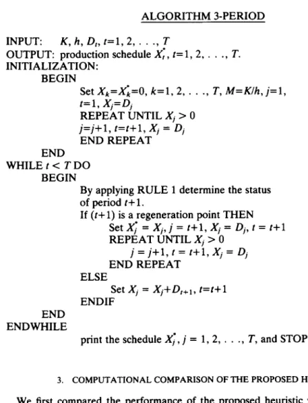
We now give the statement of the algorithm.

A L G O R I T H M 3-PERIOD

INPUT: K, h, Dr, t = l , 2 , . . . , T

OUTPUT: production schedule X~, t= 1, 2 . . . T. INITIALIZATION: BEGIN S e t X k = X k = O , k = l , 2 . . . T, M = K / h , j = I , t = l , X j = O j R E P E A T UNTIL Xj > 0 j = j + l , t = / + l , Xj = Dj END R E P E A T END WHILE t < T DO BEGIN

By applying R U L E 1 determine the status of period t + l .

If (t+ 1) is a regeneration point THEN SetX~ = X i, j = /+ l, X i = D i, t = /+ l R E P E A T UNTIL Xj > 0 j = j + I , t = / + I , X j = Dj END R E P E A T ELSE Set Xj = gj-t-Ot+l, t = t + l ENDIF END E N D W H I L E

print the schedule X~, j = 1, 2 . . . T, and STOP.

3. COMPUTATIONAL COMPARISON OF THE PROPOSED HEURISTIC

We first compared the performance of the proposed heuristic with other lot sizing heuristics, by using the standard data sets from Kaimann [22] and Berry [23]. Table 2 displays these data sets. For each data set we used five values of M = K/h. Namely, 24, 46, 60, 103 and 150.

Table 3 exhibits the results of a comparative study of nine lot sizing procedures using the end of period cost criterion. In this table we abbreviated each heuristic by their initial letters. We used G R for Groff's heuristic and G for Gaither's heuristic. 3P represents the proposed algorithm. All algorithms are programmed in F O R T R A N and run on Bur- roughs B6900 machine using B7000/B6000 F O R T R A N compiler.

The results in Table 3 show that the proposed heuristic outperforms all the other heuristic procedures over the 35 data sets used. The cumulative percent cost deviation from optimum cumulative costs for all 35 problems is 0.02% with the proposed heuristic. The cumulative percent cost deviations from the optimum cumulative costs for other heuristics are 0.35% for Gaither, 1.0% for Groff and Silver-Meal and considerably higher for the other heuristics. In 34 of 35 problems the proposed heuristic achieved the

A heuristic p r o c e d u r e for a single-item d y n a m i c lot sizing p r o b l e m Table 2. Demand data sets (Kaimann [22] and Berry [23])

187 Demand sets Period 1 2 3 4 5 6 7 1 92 80 50 10 0 0 80 2 92 100 80 10 0 0 100 3 92 125 180 15 0 0 125 4 92 100 80 20 0 25 100 5 92 50 0 70 0 100 270 6 92 50 0 180 1105 300 50 7 92 100 180 250 0 400 230 8 92 125 150 270 0 250 0 9 92 125 10 230 0 30 50 10 92 100 100 40 0 0 0 11 92 50 180 0 0 0 40 12 93 100 95 10 0 0 60 Total 1105 1105 1105 1105 1105 1105 1105 Standard deviation 0.0 27.0 66.1 130.0 305.0 136.2 79.2 Co¢ff. of variation 0.0 0.293 0.718 1.410 3.310 1.480 0.870

optimum solution whereas Gaither achieved 31, Groff achieved 28 and Silver-Meal achieved 27 optimal solutions. The other heuristics were considerably inferior.

Also in Table 3 we have shown the cumulative CPU seconds for 35 problems. As expected all the heuristics being one-pass algorithms require approximately same time. However, as expected, the time required for Wagner and Whitin algorithm was 3-5 times higher than all heuristics considered.

As indicated by Silver [19] and Gaither [20] the quality of solutions of many heuristics deteriorates as M=K/h and T become large. We have observed the similar results in our proposed heuristic as well. The algorithm tends to accumulate more than necessary number of periods for each production run. To help overcome this deficiency we have used the following modified criterion for testing of period t + l is a regeneration point:

R U L E 2. If K ~> 2 ( t - j + 1 ) Dt+l + ( t - j + 2 ) Dt+2 or if R U L E 1 is satisfied then period t + l is a regeneration point. Otherwise, period t + l is not a regeneration point.

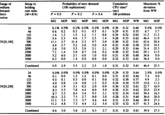
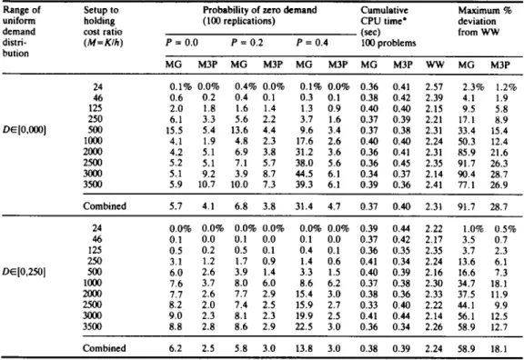
Considering the success of modified Gaither's heuristic [20] over Silver and Meal [12] and Groff [13], we decided to compare our modified algorithm to modified Gaither's on 24,000 randomly generated problems. We designed the experiments as follows: for the decision Horizon T, we have used 12, 24, 36 and 48 periods. For M=K/h we have used 24, 46, 125,250, 500, 1000, 2000, 2500, 3000 and 3500. Demand is generated uniformly between 0 and 100 and also between 0 and 250. Moreover, for each problem, after the demand data is generated we have randomly set P x 100% periods demands to zero. We have used 0.0, 0.2 and 0.4, for P values. For each combination of T, M, D and P we have replicated the experiment 100 times. All algorithms are coded in F O R T R A N and tests on a VAX 11/750 computer.

Tables 4, 5, 6, and 7 summarize the results of these experiments. In these tables MG represents "modified Gaither" and M3P represents "modified 3P" and WW represents Wagner and Whitin algorithms. The last two columns in these tables represent the maximum deviation of MG and M3P from WW (in terms of objective function value) out of 300 problems solved (100 replication for each P-value). Columns 9, 10 and 11 represent cumulative CPU times in seconds of 100 problems in the given D and M combination. (Cumulative CPU seconds of 300 problems divided by 3.) All times reported are on VAX 11/750 by using F O R T R A N compiler in a time sharing mode. Columns 3-8 represent the cumulative percent deviation of each algorithm from WW

188 O. S. B ~ N u et al.

Table 3. Comparison of eight heuristic algot~thml a n d W a g n e r - W h i t i n Algorithm on 35 d e m a n d s e a taken from X m m a n n [22] a n d Berry [23]

Algoritlum

D e m a n d Setup to

set holding

number cost ratio

(M=K/h) E O Q P O Q L U C PPB SM G R G 3P W W 24 0% 0% 0% 0% 0% 0% 0% 0% 0% 46 0 0 0 41.7 0 0 0 0 0 1 60 74.0 0 0 26.8 0 0 0 0 0 103 38.0 0 0 0 0 0 0 0 0 150 38.1 0 0 0 0 0 0 0 0 Worst ease 38.1 0 0 41.7 0 0 0 0 0 24 24.0 0 0 0 0 0 0 0 0 46 63.9 0 0 14.5 0 0 0 0 0 2 60 41.4 0 7.1 24.3 0 0 0 0 0 103 67.6 6.1 0 6.1 8.4 4.2 4.2 0 0 150 46.8 0 3.4 3.4 0 0 0 0 0 Worst case 67.6 6.1 7.1 24.3 8.4 4.2 4.2 0 0 24 51.3 6.2 39.8 0 0 0 0 0 0 46 76.4 8.5 21.2 16.0 0 0 0 0 0 3 60 97.3 9.1 20.0 13.6 0 0 0 0 0 103 49.6 15.5 13.7 15.5 0 0 0 0 0 150 65.1 7.7 13.3 7.7 0 0 0 0 0 Worst case 97.3 15.5 39.8 16.0 0 0 0 0 0 24 63.6 9.1 1.7 8.3 1.7 1.7 0 0 0 46 85.4 21.0 14.4 12.9 4.8 7.2 1.0 1.0 0 4 60 92.3 26.9 13.5 3.8 1.9 7.7 11.5 0 0 103 67.6 44.4 16.5 9.8 1.3 1.3 0 0 0 150 75.7 33.6 21.5 0 0 0 0 0 0 Worst case 92.3 44.4 21.5 12.9 4.8 7.7 11.5 1.0 0 24 0 0 0 0 0 0 0 0 0 46 0 0 0 0 0 0 0 0 0 5 60 0 0 0 0 0 0 0 0 0 103 0 0 0 0 0 0 0 0 0 150 0 0 0 0 0 0 0 0 0 Worst case 0 0 0 0 0 0 0 0 0 24 138.2 0 0 4.2 0 0 0 0 0 46 150.0 6.2 26.9 0 0 0 0 0 0 6 60 150.0 18.2 21.2 12.1 0 0 0 0 0 103 98.0 54.8 13.5 0 0 0 0 0 0 150 102.2 14.9 78.1 30.1 0 0 0 0 0 Worst case 150.0 54.8 78.1 30.1 0 0 0 0 0 24 60.8 0 0 0 0 0 0 0 0 46 28.7 0 3.0 8.3 0 0 0 0 0 7 60 45.8 1.7 30.5 20.3 0 0 0 0 0 103 65.8 0.3 59.8 0 0.3 0.3 0 0 0 150 57.6 4.3 20.7 0 4.3 6.0 0 0 0 Worst case 65.8 4.3 59.8 20.3 4.3 6.0 0 0 0 Cumulative objective value (35problems) 65568 44790 46266 44416 41148 41134 4 ~ 8 8 40754 40746 % deviation from optimum (35 problems) 60.9 9.9 13.5 9.0 1.0 1.0 0.35 0.02 0.0 CPU seconds* (35problems) 0.045 0.045 0.036 0.042 0.036 0.046 0.048 0.037 0.149 No. of optimal solutions (35 problems) 7 16 15 15 27 28 31 34 35

A heuristic p r o c e d u r e for a single-item d y n a m i c lot sizing p r o b l e m 189 Table 4. Results of 12 period problen~. (Entries in columns 3--8 represent cumulative percent deviation of total costs of each

heurhtic from the WW optimal costs for 100 replications)

Range of Setup to Probability of zero demand Cumulative Maximum %

uniform holding (100 replications) CPU time" deviation

demand cost ratio (zec) from WW

distri- ( M = K I h ) P = 0 . 0 P = 0.2 P = 0.4 100 problems bution MG M3P MG M3P MG M3P MG M3P WW MG M3P DE[0,100] 24 46 0.6 0.2 125 1.6 1.3 250 5.4 2.3 500 11.1 3.7 11300 4.9 2.7 2000 5.8 5.0 2500 7.1 1.4 3000 5.2 0.0 3500 6.3 0.0 0.1% 0.0% 0.2% 0.0% 0.2% 0.0% 0.30 0.32 0.60 9.4% 0.0% 0.5 0.1 0.5 0.1 0.29 0.31 0.55 8.7 5.7 1.5 1.2 1.1 0.8 0.34 0.32 0.63 !1.2 11.2 4.6 1.7 2.5 1.4 0.28 0.33 0.62 46.4 11.9 11.4 3.3 9.7 2.0 0.30 0.32 0 . 6 1 43.6 20.4 5.2 2.6 5.0 4.0 0.32 0.30 0.58 33.0 19.5 5.5 3.9 3.1 2.1 0.29 0.33 0.64 31.4 25.3 5.0 0.7 2.6 0.2 0.30 0.32 0.62 29.1 11.5 3.1 0.0 1.0 0.0 0.31 0.30 0.60 34.6 0.0 1.4 0.0 0.0 0.0 0.32 0.33 0.61 36.4 0.0 Combined 6.9 2.9 5.5 2.2 2.5 1.0 0.31 0.32 0 . 6 1 46.4 25.3 24 0.0% 0.0% 0.0% 0.0% 0.0% 0.0% 0.29 0.35 0.64 2.9% 0.0% 46 125 250 5OO 1000 200O 250O 3000 350O D~[0,250] 0.1 0.0 0.5 0.1 4,0 0.8 5.0 1.9 8.3 5.3 8.7 3.3 10.3 2.2 11.1 3.5 11.2 4.8 1.5 1.2 0.1 0.0 0.31 0.32 0.66 7.4 0.0 0.3 0.0 0.1 0.0 0.32 0.30 0.57 9.9 2.5 1.6 0.8 1.3 0.5 0.34 0.34 0.55 15.8 11.3 3.1 0.2 2.0 0.9 0.30 0.32 0 . 6 1 22.7 16.9 7.8 4.4 8.0 5.0 0.30 0 . 3 1 0.62 33.0 23.9 8.4 3.4 9.5 3.1 0.32 0.34 0.63 39,4 16.5 7.5 2.7 8.0 3.0 0.28 0 . 3 1 0.60 36.0 20.0 7.3 3.7 4.6 4.0 0.31 0.33 0.66 39.9 27.5 7.3 4.4 3.2 5.4 0.33 0.32 0.57 41.5 24.6 Combined 6.6 3.0 5.8 2.5 6.3 2.7 0.31 0.32 0.61 39.9 27,5

* All times are on VAX 11/750 using FORTRAN Compiler.

TaMe 5. Results of 24 period problems. (Entries in columns 3--8 represent cumulative percent deviation of total costs of each heuristic from the WW optimal costs for 100 replications)

Range of uniform demand distri- bution

Setup to Probability of zero demand Cumulative Maximum %

holding (100 replications) CPU time* deviation

cost ratio (see) from WW

( M = K / h ) P - 0.0 P = 0.2 P = 0.4 100 problems MG M3P MG M3P MG M3P MG M3P WW MG M3P DEI0,100] 24 46 125 250 500 1000 2000 3000 3500 0.1% 0.0% 0.1% 0.0% 0.1% 0.0% 0.30 0.40 1 . 4 9 4.1% 0.5% 0.6 0.1 0.4 0.1 0.4 0.1 0.32 0.35 1.29 4.1 4.3 2.0 1.7 1.4 1.5 1.0 0.9 0.35 0.37 i.15 11.3 6.3 6.7 2.7 5.4 2.1 4.0 1.9 0.28 0.33 1.20 26.6 11.4 14.7 4.8 13.6 3.6 10.3 3.2 0.32 0.36 1.30 39,7 19.2 4.0 2.5 6.4 2.5 13.6 3.0 0.31 0.37 1.17 57.5 13.7 5.8 5.0 6.4 3.9 23.6 3.0 0.36 0.39 1.22 62,5 19.8 7.1 1.4 5.7 3.9 17.2 5.2 0.33 0.32 1.30 46.0 31.8 4.0 6.8 3.9 8.7 11.4 g.l 0.29 0.35 1.32 37.0 31.8 5.2 13.4 5.9 14.3 8.1 10.2 0.34 0.34 1,20 41.3 38.9 Combined 6.6 3.0 6.5 3.2 13.0 5.8 0.32 0.36 1.26 62.5 38.9 D~[0,250i 24 46 125 250 500 1000 200O 25O0 30O0 3500 0.0% 0.0% 0.0% 0.0% 0.0% 0.0% 0.34 0.36 1.19 1.2% 0.7% 0.1 0.0 0.1 0.0 0.1 0.0 0.33 0.35 1.23 3.6 1.0 0.6 0.2 0.5 0.1 0.3 0.1 0.27 0.39 1.35 4.4 2.2 3.4 1.1 1.7 0.8 1.5 0.5 0.36 0.32 1.42 13.2 8.0 5.7 2.5 3.6 1.7 2.4 1.3 0.35 0.34 1.12 16.5 10.3 7.3 5.7 8.6 6.2 8.1 6.0 0.29 0,35 1.21 24.4 18.0 7.7 2.3 8.0 3.4 12.7 3.3 0.33 0.32 1.30 38.9 13.9 8.1 2.2 8.3 3.0 14.2 3.0 0.34 0.34 1.26 58.7 17.1 9.2 3.3 9.5 2.9 17.8 2.5 0.30 0.37 1.30 57.7 14.3 9.4 2.9 9.0 2.7 21.0 3.1 0.36 0.39 1.20 66.6 14.9 Combined 6.1 2.9 6.0 3.3 12.4 3.1 0.33 0.35 1.26 66.6 18.0

190 O . S . BENLI el al.

Table 6. Results of 36 period problems. (Entries in columns 3--8 represent cumulative percent deviation of total costs of each heuristic from the W W optimal costs for 100 replications)

Range of Setup to Probability of zero d e m a n d Cumulative Maximum %

uniform holding (100 replications) CPU time" deviation

d e m a n d cost ratio (sec) from W W

distri- ( M = K / h ) P = 0.0 P = 0.2 P = 0.4 100 problems bution M G M3P M G M3P M G M3P M G M3P WW MG M3P DEI0,000] 24 0.1% 0.0% 0.4% 0.0% 0.1% 0.0% 0.36 0.41 2.57 2.3% 1.2% 46 0.6 0.2 0.4 0.1 0.3 0.1 0.38 0.42 2.39 4.1 1.9 125 2.0 1.8 1.6 1.4 1.3 0.9 0.40 0.40 2.15 9.5 5.8 250 6.1 3.3 5.6 2.2 3.7 1.6 0.37 0.39 2.21 17.1 8.9 500 15.5 5.4 13.6 4.4 9.6 3.4 0.37 0.38 2.31 33.4 15.4 I000 4.1 1.9 4.8 2.3 17.6 2.6 0.40 0.40 2.24 50.3 12.4 2000 4.2 5.1 6.9 3.8 31.2 3.6 0.36 0.41 2.31 85.9 21.6 2500 5.2 5.1 7.1 5.7 38.0 5.6 0.36 0.45 2.35 91.7 26.3 3000 5.1 9.2 3.9 8.7 44.5 6.1 0.34 0.37 2.14 90.4 28.7 3500 5.9 10.7 10.0 7.3 39.3 6.1 0.39 0.36 2.41 77.1 26.9 Combined 5.7 4.1 6.8 3.8 31.4 4.7 0.37 0.40 2.31 91.7 28.7 DE[0,250] 24 0.0% 0.0% 0.0% 0.0% 0.0% 0.0% 0.39 0.44 2.22 1.0% 0.5% 46 0.1 0.0 0.1 0.0 0.1 0.0 0.37 0.42 2.17 3.5 0.7 125 0.5 0.2 0.5 0.1 0.4 0.1 0.36 0.35 2.35 3.7 2.3 250 3.1 1.2 1.7 0.9 1.4 0.6 0.41 0.34 2.24 13.6 6.1 500 6.0 2.6 3.9 1.4 3.3 1.5 0.40 0.39 2.16 16.6 7.3 1000 7.6 3.7 8.0 6.0 8.6 6.2 0.37 0.38 2.30 34.7 18.1 2000 7.7 2.6 7.7 2.9 15.4 3.0 0.38 0.36 2.33 37.5 11.9 2500 8.2 2.0 7.4 2.5 15.9 2.7 0.33 0.40 2.22 44.1 9.9 3000 9.0 2.3 8.1 2.3 19.9 2.5 0.41 0.44 2.14 56.1 12.5 3500 8.8 2.8 8.6 2.9 22.5 3.0 0.36 0.34 2.26 58.9 12.7 Combined 6.2 2.5 5.8 3.0 13.8 3.0 0.38 0.39 2.24 58.9 18.1

* All times are on V A X 11/750 using F O R T R A N Compiler.

Table 7. Results of 48 period problems. (Entries in columns 3-8 represent cumulative percent deviation of total costs of each heuristic from the W W optimal costs for 100 replications)

Range of uniform d e m a n d distri- bution

Setup to Probability of zero d e m a n d Cumulative Maximum %

holding (100 replications) CPU time* deviation

cost ratio (sec) from W W

( M = K / h ) P = 0.0 P = 0.2 P = 0.4 100 problems M G M3P M G M3P M G M3P M G M3P W W M G M3P DE[0,2501 24 0.1% 0.2% 0.1% 0.0% 0.1% 0.0% 0.48 0.53 4.33 1.9% 0.9% 46 0.5 0.2 0.4 0.1 0.3 0.1 0.42 0.54 4.17 4.1 4.1 125 2.1 1.8 1.7 1.4 1.2 1.0 0.46 0.44 3.97 7.7 5.7 250 6.1 3.3 5.2 2.4 3.9 2.0 0.50 0.47 4.25 14.8 8.0 500 16.5 4.8 13.8 4.3 10.6 3.6 0.47 0.49 4.13 32.3 14.4 1000 4.0 1.8 4.1 2.4 20.6 3.3 0.52 0.60 4.24 56.2 12.9 2000 4.8 4.7 4.3 4.8 31.9 4.1 0.44 0.59 3.95 69.4 18.3 2500 4.9 5.5 7.3 5.2 33.9 5.7 0.43 0.47 4.30 98.9 24.6 3000 5.0 8.7 8.6 7.2 41.7 6.6 0.46 0.49 4.40 96.8 21.2 3500 6.2 9.1 11.1 8.7 51.8 7.7 0.48 0.52 4.30 122.9 35.3 Combined 5.8 4.0 6.0 4.0 33.2 5.3 0.47 0.52 4.20 122.9 35.3 DE[0,2501 24 0 . 1 % 0 . 0 % 0 . 0 % 0 . 0 % 0 . 0 % 0 . 0 % 0.50 0.62 3.95 1.1% 0 . 8 % 46 0.1 0.0 0.1 0.0 0.1 0.0 0.49 0.44 4.17 3.2 0.5 125 0.6 0.2 0.5 0.1 0.3 0.1 0.55 0.51 4.32 3.2 1.8 , 250 2.6 1.2 1.6 0.9 1.3 0.5 0.40 0.49 4.26 10.7 4.4 500 5.9 2.7 4.4 1.7 3.6 1.8 0.43 0.46 3.89 15.9 8.3 1000 8.0 6.6 8.7 6.6 8.9 6.1 0.44 0.52 4.41 22.5 15.3 2000 7.0 2.3 9.0 2.8 16.0 3.0 0.47 0.57 4.17 45.0 11.0 2500 7.1 1.9 8.3 2.4 18.9 2.9 0.50 0.47 3.98 47.27 11.8 3000 7.9 2.3 8.6 2.7 22.8 2.7 0.46 0.49 4.22 65.8 10.5 3500 7.6 2.5 8.5 2.6 25.6 2.9 0.40 0.56 4.31 68.8 11.3 Combined 5.9 3.1 6.6 3.1 15.0 3.0 0.46 0.51 4.17 68.8 15.3

A heuristic procedure for a single-item dynamic lot sizing problem 191 algorithm for 100 replications. The rows designated as "combined" shows the cumulative percent deviation of each algorithm from WW algorithm for a given D and P combin- ation. We note here that each entry in the combined row under columns 3--8 represents the cumulative deviation of 1000 problems.

We can summarize some of the important results of this experimentation as follows:

• Both algorithms MG and M3P require approximately same CPU time, whereas WW algorithm requires 2 (for 12 period problems) to 5 (for 48 period problems) times more CPU time. This result was expected since both MG and M3P are O(T) algorithms whereas WW is an O ( T 2) algorithm.

• The proposed M3P algorithm is clearly superior to MG algorithm.

• Out of 24,000 problems solved by each algorithm in the worst case MG deviated from WW solution by 122.9% whereas M3P deviated from WW solution by 38.9%. • The cumulative percent deviation of M3P from WW for 1000 problems (for a given T,

D and P combination and for all M values) ranged between 1% (for DE[0,250], T = 12, P = 0.0 and for all M values) and 5.8% (for DE[0,100), T = 24, P = 0.4, and for all M values). This range was between 2.5% (for D~[0,100], P = 0.4, T = 12 and for all M values) and 33.2% (for DE[0,100], P = 0.4, T = 48 and all M values) for the MG algorithm.

• No dramatic degradation is observed for both algorithms for 12 period problems for all values of D, P, and M.

• Slight degradation is observed for both algorithms for 24 period problems. This degradation became more visible for P = 0.4 in both algorithms. However, degrada- tion was more severe for MG than M3P.

• The degradation of MG became quite serious for 36 period problems with P = 0.4 and M I> 2000. In contrast, no further degradation is observed in M3P.

• The degradation of MG continued for 48 period problems, especially for P = 0.4 and M >I 2000. In contrast, no further degredation is observed in M3P.

4. CONCLUSIONS

A simple heuristic procedure for SIDLS problems is introduced in this paper. The algorithm compares very favorably with the existing heuristic procedures. The algorithm is based on the concept of regeneration points in an optimal solution. The algorithm tries to establish these regeneration points by using a simple rule obtained from a 3-period analysis.

Since the proposed algorithm is a one-pass algorithm and since for each t = 1, 2 . . . . , T a constant number of operations are performed, the complexity of the proposed algorithm is of O(T).

The proposed algorithm compares quite favorably with Modified Gaithers heuristic. Out of 24,000 problems solved, in the worst case the deviation of the proposed heuristic from the optimal Wagner-Whitin solution was 38.9%. The results of the proposed algorithm indicated that it is robust. No serious degradation occurs in overall perform- ance with increased P, T, or K/h values.

Acknowledgements--The authors wish to thank the referees for their valuable input. Especially one referee's suggestions on establishing RULE 2 have improved the paper and the robustness of the algorithm considerably.

REFERENCES

1. G. T. Bishop. On a problem of production scheduling. Ops Res. $, 97-103 (1957).

2. E. H. Bowman. Production scheduling by the transportation method of linear programming. Ops Res. 4,

100-103 (1956).

3. S. S. Erenguc and S. Tufekci. A Transportation Type Aggregate Production Model with Bounds on Inventory and Backordering. Department of Industrial and Systems Engineering, University of Florida, Research Report No. 84-29, 1984.

192 O . S . BENLI et al.

4. S. M. Johnson. Sequential production planning over time at minimum cost. Mgmt Sci. 3, 1295--1300 (1957).

5. E. M. Posner and W. Szwarc. Transportation type aggregate production model with backordering. Mgmt Sci. 29, 188-199 (1983).

6. A. F. Veniott Jr. Production planning with convex costs: a parametric study. Mgmt Sci. 10, 441-460

(1964).

7. H. M. W a g n e r and T. M. Whitin. Dynamic version of the economic lot size model. M g m t Sci. 5, 89--96 (1958).

8. S. S. Ercnguc and S. Tufckci. A branch-and-bound algorithm for a singlc-itcm multi-source dynamic lot- sizing problem with capacity constraints, lie Trans. In press.

9. M. Florian and M. Klein. Deterministic production planning with concave costs and capacity constraints.

Mgmt Sci. 18, 12-20 (1971).

10. R. Jaganathan and M. R. Rao. A class of deterministic production planning problems. Mgmt Sci. 19,

1295-1300 (1973).

11. N. A. Gaither. A near-optimal lot-sizing model for requirements planning systems. Production Inventory Mgmt 22, 75-89 (1981).

12. E. A. Silver and H. C. Meal. A heuristic for selecting lot size quantities for the case of a deterministic time-varying demand rate and discrete opportunities for replenishment. Production Inventory Mgmt 14,

64--74 (1973).

13. G. K. Groff. A lot-sizing rule for time-phased component demand. Production Inventory Mgmt 20, 47-53 (1979).

14. J. J. DeMatteis. An economical lot sizing technique: part period algorithm. IBM System J. 7, 3038 (1968). 15. R. J. Tersine. Principles of Inventory and Materials Management, 2nd Ed. North Holland, Amsterdam

(1982).

16. J. Orlicky. Materials Requirement Planning. McGraw Hill, New York (1975). 17. S. Axsater. Worst case performance for lot sizing heuristics. EIOR 9, 339-343 (1982).

18. E. A. Silver and J. Miltenburg. Two modifications of the Silver-Meal lot sizing heuristic. INFOR 22, 56-59

(1984).

19. E. A. Silver. Comments on 'a near-optimal lot sizing model'. Production Inventory Mgmt 3rd Ouarter, 115-116 (1983).

20. N. Gaither. An improved lot-sizing model for MRP systems. Production Inventory Mgmt 3rd Quarter, 10- 20 (1983).

21. L. A. Johnson and D. C. Montgomery. Operations Research in Production Planning, Scheduling and Inventory Control. Wiley, New York (1974).

22. R. A. Kaimann. EOQ vs dynamic programming---which one to use for inventory ordering. Production Inventory Mgmt 4th Quarter, 66-74 (1969).

23. W. L. Berry. Lot-sizing procedures for requirement planning systems: framework for analysis. Production Inventory Mgmt 2nd Ouarter, 19-34 (1972).

24. J. Blackburn and R. Millen. Heuristic lot sizing performance in a rolling schedule environment. Decis. Sci.