Enhancing higher harmonics of a tapping cantilever by excitation at a submultiple
of its resonance frequency
M. Balantekin*and A. Atalar
Bilkent University, Electrical Engineering Department, Bilkent, TR-06800, Ankara, Turkey
共Received 24 May 2004; revised manuscript received 25 October 2004; published 22 March 2005兲 In a tapping-mode atomic force microscope, the frequency spectrum of the oscillating cantilever contains higher harmonics at integer multiples of the excitation frequency. When the cantilever oscillates at its funda-mental resonance frequency w1, the high Q-factor damps the amplitudes of the higher harmonics to negligible levels, unless the higher flexural eigenmodes are coincident with those harmonics. One can enhance the nth harmonic by the Q factor when the cantilever is excited at a submultiple of its resonance frequency 共w1/ n兲. Hence, the magnitude of the nth harmonic can be measured easily and it can be utilized to examine the material properties. We show theoretically that the amplitude of enhanced higher harmonic increases monotonically for a range of sample stiffness, if the interaction is dominated by elastic force.
DOI: 10.1103/PhysRevB.71.125416 PACS number共s兲: 68.37.Ps, 62.20.Dc
I. INTRODUCTION
The determination of sample elasticity at a nanometer scale has been a goal of many researchers.1–16 The nanoindentation,1 force modulation,2 atomic force acoustic
microscopy,3 or ultrasonic force microscopy4 are the
meth-ods developed so far to characterize the local elastic proper-ties of samples. In these methods, the applied static loads degrade the lateral resolution.
It was recently found that the anharmonic oscillations of the cantilever contain information about the material na-nomechanical properties.17–20 Hillenbrand et al. used the
13th harmonic signal to increase the image contrast.18 Some
authors used second and third harmonic amplitudes to map the surface charge density of DNA molecules.21 Dürig
real-ized that the higher harmonic amplitudes can be utilreal-ized for the reconstruction of the interaction force.22 A numerical
analysis by Rodriguez and Garcia showed that phase of the second mode can be utilized to map the Hamaker constant.23
Since the tip-sample interaction is periodic, the frequency spectrum of the detected signal has components共harmonics兲 at integer multiples of the driving frequency. These harmon-ics depend on the interaction force and hence the material properties.
In conventional tapping-mode experiments, the higher harmonics are generally ignored and in fact, their amplitudes are two or three orders of magnitude smaller than the funda-mental component of oscillation as both numerical24 and experimental25results indicate. The nth harmonic amplitude
is related to the nth harmonic of the interaction force fn via
the transfer gain兩H共nw兲兩 as follows:
An=兩H共nw兲fn兩, for n 艌 2, 共1兲 where w is the excitation frequency. The transfer function of a rectangular cantilever including higher flexural eigenmodes was obtained by Stark and Heckl.17
To increase the nth harmonic amplitude Anand hence the
measurement sensitivity, we must increase either fn or 兩H共nw兲兩. Notice that increasing fn may mean an additional
damage to the sample, and therefore it may not be desirable
for all kinds of samples. The transfer gains for the higher harmonics in conventional tapping-mode operation 共w=w1, where w1 is the resonant frequency of the first mode兲
are very small unless the higher harmonic frequencies are coincident with the resonant frequencies of the higher eigenmodes. If we consider only the fundamental eigenmode of a cantilever with a stiffness of k, the transfer gain for the nth harmonic will be 关k共n2− 1兲兴−1. This yields a very small value for increasing n. The use of higher harmonics close to the higher transverse resonances can enhance the measurement sensitivity.26 However, to increase the
ampli-tudes of higher harmonics in this case, one may need to increase the free oscillation amplitude or decrease the set point 共damped兲 amplitude which in turn increases the tip-sample forces.
Most cantilevers do not have eigenmodes at integer mul-tiples of each other. But, it is possible to fabricate special cantilevers, called “harmonic cantilevers,” in such a way that one of the eigenmodes is at an integer multiple of the funda-mental mode.27The recent study by Sahin et al. showed that
these cantilevers can be used to enhance one of the higher harmonics.28
Indeed, measuring the higher harmonic signal sensitivity would give an opportunity to researchers in examining the material properties at nanoscale more effec-tively. To enhance the quality of the measured harmonic signal, we propose a method which can easily be employed in conventional tapping-mode systems. In the next section, we will describe the method and test it by numerical simulations. The analytical analysis for low harmonic distor-tion is also provided in an Appendix to provide physical insight.
II. SIMULATIONS OF A NEW HARMONIC ENHANCEMENT METHOD
Considering the fundamental eigenmode, the transfer gain reaches its maximum value 共Q/k, where Q is the quality factor兲 at the first resonance frequency w1. If we drive the cantilever at a submultiple of w1, i.e., at w = w1n= w1/ n共n is
an integer number兲, then, due to the high transfer gain at nw1n= w1, the nth harmonic amplitude is expected to be
much larger than the conventional case. This allows us to detect the harmonic signal with a good signal-to-noise ratio and to inspect the tip-sample interaction effectively. To vibrate the cantilever at w1nwith a reasonable amplitude,
a higher driving force must be applied since there is no Q enhancement for the fundamental component of the oscillation.
To investigate if the proposed method can be helpful for differentiating the stiffness of materials and to analyze the effect of the method on the dynamics of tip-sample system, we performed numerical simulations. The simula-tions are done by converting the mechanical model into an equivalent electrical circuit29 containing nonlinear
elements. The equivalent circuit is simulated with SPICE, a powerful and easily available circuit simulator. The details of the simulation setup can be found elsewhere.30The
simula-tions are done in a time domain with a step size of one thousandth of one period. To make sure that the steady state is reached, 10Q oscillation cycles are simulated. We choose a typical cantilever with a stiffness of k = 1 N / m, a quality fac-tor of Q = 100, and a fundamental resonance frequency of w1= 2⫻120 krad/s. The free oscillation amplitude A0 and
set point amplitude A1 are chosen to be A0= 100 nm and A1= 0.99A0.
In tapping-mode operation, the cantilever tip experiences both attractive surface forces and a repulsive contact force. The attractive part of the interaction force contains the van der Waals and capillary forces.31If the elastic repulsive force
applied during the contact is much larger than the attractive forces, then one can ignore the attractive forces. We consid-ered only the elastic force in our simulations to find how the enhanced higher harmonics change with sample elasticity even though the attractive forces can easily be included. Ac-cording to the Hertzian contact mechanics, the normal load FHis related to the indentation depth ␦ for any kind of
in-denter as8 F
H=E*␦␣, where E* is the effective Young’s
modulus,  and ␣ are the constants dependent on the tip geometry. Usually, the tip end is approximated with a pa-raboloidal共spherical兲 shape having a radius of curvature R. In this case, the parameters defining the tip geometry will be
= 4
冑
R / 3 and ␣= 3 / 2. In the simulations R is selected to have a typical value of 10 nm.We analyzed in detail the response of the enhanced sec-ond and third harmonic signals as a function of the effective tip-sample elasticity E*, when the cantilever is driven at the
submultiple frequencies of w = w12= w1/ 2 and w = w13= w1/ 3.
Figure 1 shows the variation of normalized second共A2/ A0兲
and third共A3/ A0兲 harmonic amplitudes with E*. This figure
is divided into two regions by a dashed vertical line. In re-gion I, the tip stays in contact with the sample more than a half oscillation period, whereas in region II the contact time is less than a half period. The first observation is that the magnitude of the second harmonic signal can reach almost 40% of the fundamental component. Second, it is seen that the higher harmonic amplitudes are increasing monotonically in a certain range of sample stiffness. The second harmonic amplitude is larger than the third harmonic amplitude and the steeply increasing part of the second harmonic amplitude is
at a lower elasticity region compared to the third harmonic. Finally, we find that the tip motion can show chaotic behav-ior at a relatively high elasticity region共marked by a dotted line兲.
The phase of the cantilever oscillation can be used to map energy dissipation.32 On the other hand, it cannot be
used to differentiate the compliance of purely elastic samples.33 In such a case, the enhanced harmonic signal can be useful to increase the image contrast. To map the sample elasticity, the harmonic amplitude variations should be monotonic in a range which covers Young’s moduli of the materials under investigation. If we consider region II, it is seen that the samples which have different compliance may not be differentiated and the contrast in the images cannot be interpreted uniquely because of the nonmonotonic variations. Furthermore, there are no steady-state values of harmonic amplitudes for relatively stiff samples due to the chaotic system response. We used a time series analysis software TISEAN34 to find the largest Lyapunov exponent which indicates whether the system is chaotic or not.35 The possibility of chaotic system behavior
in conventional tapping-mode AFM was predicted by Hunt and Sarid.36 The numerical analysis by Stark37 also
showed that the chaos can occur depending on the tip-sample gap as the higher harmonics are enhanced by higher eigenmodes.
To gain further insight on the dynamics of the system response, we provided one cycle of tip position graph as obtained from the simulations for three different samples in Fig. 2. It is seen that as the sample gets stiffer, the tip motion deviates heavily from the sinusoidal shape. We can also write the power balance equation to find the relation FIG. 1. Simulation results for the second and third harmonics when the cantilever is driven at w = w1/ 2 and w = w1/ 3, respectively. A2/ A0共stars兲 and A3/ A0共asterisks兲 are plotted for a paraboloidal tip with a radius of curvature R = 10 nm. The simulation parameters are A0= 100 nm, A1/ A0= 0.99, Q = 100 and k = 1 N / m. A vertical dashed line separates the region I共␥⬍0兲 and region II 共␥⬎0兲, whereas the dotted line indicates the beginning of the chaotic region for the third harmonic. Those locations for the second harmonic are very close to these lines and not shown for clarity.
between An and the system variables. The power input
to the system is32 kw
1nAdA1sin共兲/2, where Ad and
are the drive amplitude and the phase shift between the drive and displacement signals. This power is dissipated partly by the fundamental component of tip oscillation 关kw1n
2 A 1 2/共2Qw
1兲兴 and partly by the enhanced higher
har-monic关kw12An2/共2Qw1兲兴. We assumed that there is no energy
dissipation in the sample and the other共unmatched兲 higher harmonics are negligible 共as obtained from simulations兲 since A1/ A0is set very close to 1. From this balance one can
find An in terms ofas
An=共A1/n兲关Q共n − 1/n兲共A0/A1兲sin共兲 − 1兴1/2. 共2兲
In this formulation, we used Ad⬵共1−w2/ w1 2兲A
0 which is
valid for a high-Q cantilever excited at w艋w1/ 2. It is found
that Ananddepend on each other. We observed in
simula-tions that initially increases and after a peak value it de-creases as the sample gets stiffer. This explains the non-monotonic behavior seen in Fig. 1. Equation共2兲 also helps to explain the observed amplitude differences in second and third harmonics. For a given w1, as n increases the energy
input decreases which in turn limits the amplitude of the nth harmonic.
If the higher harmonic signal An becomes a significant
fraction of A0, the relation between Anand the sample
stiff-ness is no longer monotonic. Moreover, the cantilever can get into chaotic motion if the sample stiffness is very high. To avoid these problems, the enhancement can be reduced by choosing an excitation frequency that is slightly different than the submultiple frequency.
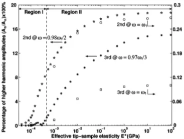
We performed the simulations at slightly shifted excita-tion frequencies and plotted the results in Fig. 3. For the second harmonic we drive the cantilever at w = 0.98w12
and for the third harmonic we selected w = 0.97w13. It is
seen that the variations become monotonic in region II and the chaotic behavior is eliminated. The amplitudes
saturate for increasing sample stiffness. The saturated ampli-tudes of second and third harmonics are still more than 15% of A0 which gives a very good sensitivity. To make a
comparison between the harmonic amplitudes of the conven-tional mode of operation, where the cantilever is excited at w = w1, we performed more simulations and plotted the re-sults in the same figure. We find that the second and third harmonic amplitudes in the conventional case are not more than 0.3% of A0.
The force applied by the tip on the surface must be carefully chosen for imaging delicate samples. For the same cantilever and tip shape, the parameters that affect the interaction force are the driving frequency38,39 w, free
oscillation amplitude A0, and the set point ratio A1/ A0. To
enhance the second harmonic, we excite the cantilever at 0.98w12. A0 and A1/ A0 are selected to be 100 nm and
0.99. For the selected parameters, we found that the maximum value of the interaction force is less than 18 nN for the elasticity of samples less than 10 GPa. As a compari-son, the maximum applied force is found to be less than 17.6 nN in conventional tapping mode operation 共w=w1兲 with the parameters of A0= 100 nm and A1/ A0= 0.6
and for the same range of sample elasticity. Note that the force applied to the surface in a conventional case will be less than 5.5 nN if we select A1/ A0= 0.99, in which case the
higher harmonic amplitudes will be less than 0.05% of A0.
Here, we selected A1/ A0to be 0.6 to make a fair comparison
between the higher harmonic amplitudes of two cases. Hence, we conclude that higher harmonic amplitudes of the proposed method are much larger than that of the conven-tional case even though the same forces are applied to the surface.
III. CONCLUSIONS
We showed that the higher harmonic amplitudes can be enhanced by exciting the cantilever at a submultiple of fun-FIG. 2. Tip motions taken from simulations for three different
elastic samples when the cantilever is excited at w = w1/ 2. The po-sition of the undeformed sample surface is indicated by the hori-zontal line.
FIG. 3. Left-hand axis: Simulation results for A2
共w=0.98w1/ 2兲 marked by stars and A3共w=0.97w1/ 3兲 marked by asterisks in the percentage of A0with the same parameters of Fig. 1. The vertical dashed line indicates the ␥=0 location. Right-hand axis: Simulation results for the conventional case 共w=w1兲. A2 is marked by circles and A3is marked by rectangles in the percentage of A0at A1/ A0= 0.6. The other parameters are the same.
damental resonance. With this method, the most sensitive portion of the cantilever transfer function is utilized for the detection of harmonic amplitudes. We demonstrated that the amplitude of the enhanced higher harmonics is almost monotonically related to sample elasticity. In tapping-mode operation, the lateral forces are reduced significantly and therefore harmonic imaging offers a higher image resolution compared to the previously developed elasticity imaging methods.
APPENDIX: ANALYTICAL APPROXIMATION FOR LOW HARMONIC DISTORTION
In tapping-mode operation, as the tip taps on an elastic sample, it indents periodically into the sample during the contact. If we assume that the sinusoidal nature of the tip motion is preserved 共low harmonic distortion兲, then the in-dentation depth is also sinusoidal in the contact duration. For a given set point amplitude A1, mean tip to surface
sepa-ration zr and excitation frequency w, we can express the
time-dependent interaction force fTS共t兲 in one period if 兩zr兩艋A1 as
fTS共t兲 =
再
E *关A1cos共wt兲 − zr兴␣ for 兩t兩 艋 cos−1共zr/A1兲/w
0, otherwise.
冎
共A1兲 If zr⬎A1 then fTS共t兲=0 and if zr⬍−A1 then fTS共t兲 =E*关A
1cos共wt兲−zr兴␣.
For a tip having a conical shape, the parameter defining the tip geometry is the semivertical angle 关= 2 tan共兲/,
␣= 2兴. Defining a normalized mean tip to surface distance␥ as ␥= zr/ A1, the maximum force applied to the sample is
found to be
Fmax= 2 tan共兲E*A1
2共1 −␥兲2/. 共A2兲
In the steady state, the interaction force can be expanded in a Fourier series17,40 as f
TS共t兲= f0+兺n艌1fncos共nwt兲. For
兩␥兩艋1, the average force f0 is given by f0= Fmax
0.5 +␥2+ 0.5 sinc共2兲 − 2␥sinc共兲
共1 −␥兲2 , 共A3兲
where sinc共x兲,sin共x兲/共x兲. = cos−1共␥兲/ is the
normal-ized contact time, i.e., the contact time divided by one period 共w/ 2兲. The fundamental and higher order force compo-nents are found using
fn= 2Fmax hn共␥兲
共1 −␥兲2, 共A4兲
where hn共␥兲 is given by
hn共␥兲 = −␥兵sinc关共1 + n兲兴 + sinc关共1 − n兲兴其 + 共0.5 +␥2兲
⫻sinc共n兲 + 0.25兵sinc关共2 + n兲兴 + sinc关共2 − n兲兴其. 共A5兲 f1 causes an amplitude damping30 and can be related
to oscillation amplitude and cantilever parameters under the assumption of low harmonic distortion as follows:
f1= A1共w兲兩H共w兲兩−1, 共A6兲
where
共w兲 = 兵共A0/A1兲
2− sin2关⬔H共w兲兴其1/2− cos关⬔H共w兲兴,
共A7兲 and the transfer function of a fundamental flexural eigen-mode of the cantilever is
H共w兲 =Q k 共1 − w2/w 1 2兲Q − iw/w 1 共1 − w2/w 1 2兲2Q2+ w2/w 1 2, 共A8兲
here k, Q, A0, and w1 are the cantilever stiffness, quality
factor, free oscillation amplitude, and fundamental resonant frequency, respectively. Equations 共A4兲 and 共A6兲 tell us that for any given set of cantilever parameters and a set point amplitude, Fmax and are almost inversely
propor-tional.
Equations共A2兲 and 共A4兲 must be satisfied simultaneously. Therefore, we plot Fmax/共A1␣E兲 and Fmax/ f as a function
of ␥ for differing values of E* and f1 in Fig. 4 to
find a solution for a given sample elasticity. Here, E and f =A1␣E are the arbitrary values of E*and f
1. An intersection
of the curves gives the solution for ␥ and Fmax values
for a specific sample and a cantilever. No intersection means that there is no solution for the chosen cantilever. When
␥⬍−1, it is found that f0= Fmax共0.5+␥2兲/共1−␥兲2, f1= −2Fmax␥/共1−␥兲2, f2= 0.5Fmax/共1−␥兲2 and fn艌3= 0.
Actually, f1 is given by −4 tan共兲E*A 1
2␥/ which increases
for decreasing ␥ and hence there is always an intersection point.
Figure 5 is a sample plot of analytical and simulation results for the tip position and the interaction force. Although the two curves are very similar, they do not match each other perfectly. Since the enhanced second harmonic amplitude is about 17.5% of A0in this case, a small harmonic amplitude
FIG. 4. Normalized maximum repulsive force Fmax/共A1␣E兲
共thin lines兲 and Fmax/ f 共thick lines兲 are plotted as a function of normalized mean tip-surface distance ␥ for varying values of E* and f1for a conical tip共␣=2兲.
approximation in an analytical derivation is violated and this deviation is to be expected. The two curves approach each other with smaller harmonic amplitudes.
Different sample elastic properties give rise to signifi-cantly different Fmaxand␥values. Although we are not able
to measure any one of these parameters directly,41 we can
extract the sample elasticity by measuring the harmonic am-plitudes. Notice that the constant term in Eq.共A1兲 depends on ␥, but the feedback signal contains information on the height variations of the sample surface also.
We can relate the effective tip-sample elasticity to the nth harmonic amplitude by combining Eqs.共A2兲 and 共A4兲 and utilizing An艌2=兩H共nw兲fn兩 as follows:
An=兩共4/兲tan共兲A1 2
H共nw兲hn共␥兲E*兩. 共A9兲
There is no direct relation between An and E* in Eq. 共A9兲.
However,or␥can be used as an independent parameter to find respective Anand E* values. We can express Anand E*
in terms of␥ only,
An=兩H共nw兲A1共w兲兩H共w兲兩−1⌳共␥兲兩, 共A10兲 where⌳共␥兲 is equal to hn共␥兲/h1共␥兲. Also E*= f1/关A1␣共␥兲兴,
where 共␥兲 is equal to 2h1共␥兲. Notice that as →0,
⌳共␥兲→1 for which An reaches its maximum value
关max共An兲兴 and 共␥兲→0 for which E*goes to infinity. In Fig.
6 we plot the first four normalized harmonic amplitudes 关An/ max共An兲=兩⌳共␥兲兩兴 as a function of the normalized
effec-tive tip-sample elasticity 关E*A 1
␣/ f
1=−1共␥兲兴 under the
as-sumption of a very small harmonic distortion 共AnⰆA1兲. In
this figure, the dashed vertical line marks the location of a
␥= 0 point.
The higher harmonic amplitudes show a monotonic in-crease in a wide range of sample compliance. Notice that the steeply increasing part of the amplitude curves shift towards a high Young’s moduli region as the harmonic number in-creases. This makes one of the higher harmonics more pref-erable than the other ones depending on the sample. As the sample gets stiffer, An saturates since the variation of the
contact time 共and the penetration depth兲 gets smaller. This imposes an upper limit for measurable sample elasticity as reported earlier.2There is also a lower limit of E*for which
␥⬎0. Both limits can be shifted to the lower side of elastic-ity by softening the lever, by increasing the set point A1/ A0
or oscillation amplitude, or by using a dull tip. The use of a dull tip is not preferable since it decreases the lateral image resolution. There is a practical maximum value of A1/ A0as
determined by the precision of the feedback electronics. The oscillation amplitude can have an upper limit. Hence, the cantilever stiffness is the most suitable parameter to adjust the measurement region. The reverse procedure can be ap-plied to shift the operation range to the high elasticity side. Note that changing these parameters also effect the maxi-mum force applied to the surface Fmax. We recall that the
attractive forces are assumed to be very small compared to Fmaxand increasing Fmaxtoo much can destroy the tip and/or
the sample. FIG. 5. Tip position and tip-sample interaction force in one
cycle for a conical tip having a semivertical angle of=15° and a sample of E*= 0.5 GPa. The thin solid lines show the analytical solutions whereas the thick dashed lines indicate the simulation results. A0= 100 nm, A1/ A0= 0.99, Q = 100, k = 1 N / m, and w = 0.98w1/ 2. Notice that the interaction force is multiplied by 10 to fit into the figure.
FIG. 6. A variation of the first four normalized harmonic ampli-tudes 兩⌳共␥兲兩 as a function of the normalized effective tip-sample elasticity −1共␥兲 for a conical tip 共␣=2兲. It is assumed that AnⰆA1. Vertical dashed and dotted lines mark the ␥=0 and
*Electronic address: [email protected]
1N. A. Burnham and R. J. Colton, J. Vac. Sci. Technol. A 7, 2906
共1989兲.
2P. Maivald, H. J. Butt, S. A. C. Gould, C. B. Prater, B. Drake, J. A. Gurley, V. B. Elings, and P. K. Hansma, Nanotechnology 2, 103共1991兲.
3U. Rabe, K. Janser, and W. Arnold, Rev. Sci. Instrum. 67, 3281
共1996兲.
4K. Yamanaka and S. Nakano, Jpn. J. Appl. Phys., Part 1 35, 3787
共1996兲.
5N. A. Burnham, A. J. Kulik, G. Gremaud, P. J. Gallo, and F. Oulevey, J. Vac. Sci. Technol. B 14, 794共1996兲.
6W. Kiridena, V. Jain, P. K. Kuo, and G. Liu, Surf. Interface Anal.
25, 383共1997兲.
7D. DeVecchio and B. Bhushan, Rev. Sci. Instrum. 68, 4498
共1997兲.
8R. W. Stark, T. Drobek, M. Weth, J. Fricke, and W. M. Heckl, Ultramicroscopy 75, 161共1998兲.
9A. Vinckier and G. Semenza, FEBS Lett. 430, 12共1998兲. 10K. Yamanaka and S. Nakano, Appl. Phys. A: Mater. Sci. Process.
66, S313共1998兲.
11A. Volodin, M. Ahlskog, E. Seynaeve, C. Van Haesendonck, A. Fonseca, and J. B. Nagy, Phys. Rev. Lett. 84, 3342共2000兲. 12E. Kester, U. Rabe, L. Presmanes, Ph. Tailhades, and W. Arnold,
J. Phys. Chem. Solids 61, 1275共2000兲.
13S. Amelio, A. V. Goldade, U. Rabe, V. Scherer, B. Bhushan, and W. Arnold, Thin Solid Films 392, 75共2001兲.
14A. Touhami, B. Nysten, and Y. F. Dufrene, Langmuir 19, 4539
共2003兲.
15T. R. Matzelle, G. Geuskens, and N. Kruse, Macromolecules 36, 2926共2003兲.
16S. Cuenot, C. Fretigny, S. D. Champagne, and B. Nysten, J. Appl. Phys. 93, 5650共2003兲.
17R. W. Stark and W. M. Heckl, Surf. Sci. 457, 219共2000兲. 18R. Hillenbrand, M. Stark, and R. Guckenberger, Appl. Phys. Lett.
76, 3478共2000兲.
19M. Stark, R. W. Stark, W. M. Heckl, and R. Guckenberger, Appl. Phys. Lett. 77, 3293共2000兲.
20O. Sahin and A. Atalar, Appl. Phys. Lett. 79, 4455共2001兲. 21S. J. T. van Noort, O. H. Willemsen, K. O. van der Werf, B. G. de
Grooth, and J. Greve, Langmuir 15, 7101共1999兲. 22U. Dürig, New J. Phys. 2, 5.1共2000兲.
23T. R. Rodriguez and R. Garcia, Appl. Phys. Lett. 84, 449共2004兲. 24T. R. Rodriguez and R. Garcia, Appl. Phys. Lett. 80, 1646
共2002兲.
25J. P. Cleveland, B. Anczykowski, A. E. Schmid, and V. B. Elings, Appl. Phys. Lett. 72, 2613共1998兲.
26R. W. Stark and W. M. Heckl, Rev. Sci. Instrum. 74, 5111共2003兲. 27O. Sahin, G. Yaralioglu, R. Grow, S. F. Zappe, A. Atalar, C. F.
Quate, and O. Solgaard, Sens. Actuators, A 114, 183共2004兲. 28O. Sahin, C. F. Quate, O. Solgaard, and A. Atalar, Phys. Rev. B
69, 165 416共2004兲.
29O. Sahin and A. Atalar, Appl. Phys. Lett. 78, 2973共2001兲. 30M. Balantekin and A. Atalar, Appl. Surf. Sci. 205, 86共2003兲. 31L. Zitzler, S. Herminghaus, and F. Mugele, Phys. Rev. B 66,
155 436共2002兲.
32B. Anczykowski, B. Gotsmann, H. Fuchs, J. P. Cleveland, and V. B. Elings, Appl. Surf. Sci. 140, 376共1999兲.
33J. Tamayo and R. Garcia, Appl. Phys. Lett. 71, 2394共1997兲. 34R. Hegger, H. Kantz, and T. Schreiber, Chaos 9, 413共1999兲. 35M. Sano and Y. Sawada, Phys. Rev. Lett. 55, 1082共1985兲. 36J. P. Hunt and D. Sarid, Appl. Phys. Lett. 72, 2969共1998兲. 37R. W. Stark, Nanotechnology 15, 347共2004兲.
38J. P. Spatz, S. Sheiko, M. Möller, R. G. Winkler, P. Reineker, and O. Marti, Nanotechnology 6, 40共1995兲.
39H. Bielefeldt and F. J. Giessibl, Surf. Sci. 440, L863共1999兲. 40M. Balantekin and A. Atalar, Phys. Rev. B 67, 193 404共2003兲. 41M. Stark, R. W. Stark, W. M. Heckl, and R. Guckenberger, Proc.
Natl. Acad. Sci. U.S.A. 99, 8473共2002兲.