Enhancing feature selection with contextual relatedness filtering using Wikipedia

ENHANCING FEATURE SELECTION WITH

CONTEXTUAL RELATEDNESS FILTERING

USING WIKIPEDIA

a thesis submitted to

the graduate school of engineering and science

of bilkent university

in partial fulfillment of the requirements for

the degree of

master of science

in

computer engineering

By

Melih Baydar

August 2017

Enhancing Feature Selection with Contextual Relatedness Filtering using Wikipedia

By Melih Baydar August 2017

We certify that we have read this thesis and that in our opinion it is fully adequate, in scope and in quality, as a thesis for the degree of Master of Science.

Fazlı Can(Advisor)

G¨onen¸c Ercan

˙Ibrahim K¨orpeo˘glu

Approved for the Graduate School of Engineering and Science:

ABSTRACT

ENHANCING FEATURE SELECTION WITH

CONTEXTUAL RELATEDNESS FILTERING USING

WIKIPEDIA

Melih Baydar

M.S. in Computer Engineering Advisor: Fazlı Can

August 2017

Feature selection is an important component of information retrieval and nat-ural language processing applications. It is used to extract distinguishing terms for a group of documents; such terms, for example, can be used for clustering, multi-document summarization and classification. The selected features are not always the best representatives of the documents due to some noisy terms. Ad-dressing this issue, our contribution is twofold. First, we present a novel approach of filtering out the noisy, unrelated terms from the feature lists with the usage of contextual relatedness information of terms to their topics in order to enhance the feature set quality. Second, we propose a new method to assess the contextual relatedness of terms to the topic of their documents. Our approach automatically decides the contextual relatedness of a term to the topic of a set of documents using co-occurrences with the distinguishing terms of the document set inside an external knowledge source, Wikipedia for our work. Deletion of unrelated terms from the feature lists gives a better, more related set of features. We evaluate our approach for cluster labeling problem where feature sets for clusters can be used as label candidates. We work on commonly used 20NG and ODP datasets for the cluster labeling problem, finding that it successfully detects relevancy in-formation of terms to topics, and filtering out irrelevant label candidates results in significantly improved cluster labeling quality.

¨

OZET

WIKIPEDIA YOLU ˙ILE BA ˘

GLAMSAL ˙IL˙IS

¸K˙I

F˙ILTRELEMES˙I KULLANARAK GEL˙IS

¸T˙IR˙ILM˙IS

¸

¨

OZELL˙IK SEC

¸ ME

Melih Baydar

Bilgisayar M¨uhendisli˘gi, Y¨uksek Lisans Tez Danı¸smanı: Fazlı Can

August 2017

¨

Ozellik ¸cıkarımı, bilgi getirimi ve do˘gal dil i¸sleme alanlarındaki uygulamalar i¸cin ¨

onemli bir bile¸sendir. Bu bile¸sen, d¨ok¨umanlar i¸cin ayırt edici kelimeler se¸cmek i¸cin kullanılır ve bu kelimeler k¨umeleme, ¸coklu d¨ok¨uman ¨ozetleme ve sınıflandırma i¸cin kullanılabilir. Se¸cilen ¨ozellikler d¨ok¨umanları i¸cin ilgisiz kelimeler olabilece˘ginden se¸cildikleri bu d¨ok¨umanları her zaman en iyi bi¸cimde temsil edemeyebilirler. Bu problemi ele aldı˘gımızda biz iki y¨onl¨u bir katkı sa˘glıyoruz. Birinci olarak, ¨ozellik gruplarının kalitesini arttırmak amacıyla kelimelerin, k¨umelerinin konularıyla arasındaki ba˘glamsal ili¸skiyi kullanarak ilgisiz kelimeleri ¨ozellik listelerinden silen yeni bir yakla¸sım sunuyoruz. ˙Ikinci olarak, kelimelerin, k¨umelerinin konularıyla arasında bir ili¸ski olup olmadı˘gına karar vermek amacıyla yeni bir y¨ontem ¨one s¨ur¨uyoruz. Y¨ontemimiz, s¨oz konusu bir kelimenin, bir d¨ok¨uman k¨umesi i¸cin ayırt edici olarak se¸cilmi¸s olan kelimeler ile dı¸s bir kaynakta beraber bulunma sayısına g¨ore ba˘glamsal olarak ili¸skili olup olmadı˘gına karar veriyor. Bu ¸calı¸smamız i¸cin dı¸s kaynak olarak Wikipedia’yı kullandık. Ozellik setlerinden ilgisiz olan ke-¨ limelerin silinmesi daha iyi ve ilgili ¨ozellik listelerinin ortaya ¸cıkmasını sa˘glıyor. Yakla¸sımlarımızı, ¨ozellik setlerinin direk olarak etiket adayı olarak kullanılabildi˘gi k¨umeleme etiketleme problemi ¨uzerinde de˘gerlendiriyoruz. Bu problem i¸cin bir¸cok kez kullanılmı¸s olan 20NG ve ODP veri setleri ¨uzerinde ¸calı¸sıyoruz. Bul-gularımıza g¨ore, ba˘glamsal ili¸ski de˘gerlendirme y¨ontemimiz ba¸sarılı bir ¸sekilde kelimelerin konularla olan ba˘glamsal ili¸ski durumunu tespit ediyor ve bu ili¸ski bil-gisi kullanılarak ilbil-gisiz kelimelerin etiket adayları arasından silinmesi k¨umeleme etiketleme kalitesini kayda de˘ger bi¸cimde geli¸stiriyor.

Acknowledgement

First, I would like to thank my advisor, Prof. Dr. Fazlı Can. I am grateful to him for his guidance, encouragement and support through my study. This thesis would not have been possible without his contributions. I am also thankful to him for the priceless conversations we had during our meetings.

I also thank to the jury members, Prof. Dr. ˙Ibrahim K¨orpeo˘glu and Assist. Prof. Dr. G¨onen¸c Ercan for reading and reviewing my thesis.

I am also appreciative of the financial, academic and technical support from Bilkent University Computer Engineering Department.

Finally, I owe my loving thanks to my precious parents and brother and my beloved fianc´ee for their undying love, support and encouragement through my life. To all my supportive friends, thank you for your understanding, encourage-ment and friendship in my life.

Contents

1 Introduction 1

1.1 Motivation . . . 3

1.2 Methodology and Contributions . . . 4

1.3 Organization of Thesis . . . 6

2 Background and Related Work 7 2.1 Feature Selection Methods . . . 7

2.1.1 Term Frequency . . . 7 2.1.2 OKAPI - BM25 . . . 8 2.1.3 Mutual Information . . . 8 2.1.4 χ2 _{Test . . . . 9} 2.1.5 Jensen-Shannon Divergence . . . 10 2.2 Cluster Labeling . . . 11 2.3 Semantic Relatedness . . . 12

CONTENTS vii

2.3.1 Lexical Resource-based Semantic Relatedness . . . 12

2.3.2 Wikipedia-based Semantic Relatedness . . . 13

3 Contextual Relatedness Filtering 18 3.1 Contextual Relatedness Assessment . . . 19

4 Experimental Setup 21 4.1 Data Collections . . . 21

4.1.1 Wikipedia Usage . . . 22

4.2 Evaluation Metrics . . . 22

4.2.1 Match@k . . . 23

4.2.2 MRR@k (Mean Reciprocal Rank@k) . . . 23

4.2.3 Statistical Test . . . 24

5 Experimental Results 26 5.1 Feature Selection Methods . . . 26

5.2 Contextual Relatedness Filtering . . . 28

6 Conclusions and Future Work 35

List of Figures

1.1 Spam folder that contains emails tagged as spam. . . 2

1.2 Google translate. . . 2

1.3 Carrot2 _{search engine. . . . . 3}

1.4 General framework of cluster labeling with contextual relatedness filtering. . . 6

2.1 Top ten Wikipedia articles in sample interpretation vectors taken from [1]. . . 15

2.2 First ten concepts of the interpretation vectors for texts with am-biguous words taken from [1]. . . 16

4.1 Clusters of ODP dataset. . . 22

4.2 Clusters of 20NG dataset. . . 23

5.1 MRR@k and Match@k results of feature selection methods on 20NG dataset. . . 27

LIST OF FIGURES ix

5.3 MRR@k and Match@k results of JSD and contextual relatedness filtering on ODP dataset. . . 28

5.4 MRR@k and Match@k results of JSD and contextual relatedness filtering on 20NG dataset. . . 29

5.5 MRR@k and Match@k results of JSD and contextual relatedness filtering on ODP dataset with different threshold and n values. . . 31

5.6 MRR@k and Match@k results of TF and contextual relatedness filtering on ODP dataset. . . 32

List of Tables

4.1 Demonstration of Match@k label quality measure calculation. BM25 method finds 8 of the clusters’ labels correctly at k=1. This leads to Match@1 = 8/20 = 0.40. On the other hand, where k=5, BM25 finds 8+2+2+0+1 = 13 of the clusters’ labels correctly which means Match@5 = 13/20 = 0.65. . . 23

4.2 Demonstration of MRR@k label quality measure calculation. BM25 method finds 8 of the clusters’ labels correctly at k=1. This leads to MRR@1 = (1/1)*8/20 = 0.40. On the other hand, where k=2, MRR@2 for BM25 is ((1/1)*8+(1/2)*2) / 20 = 0.45 which means BM25 finds correct labels for clusters at 2.22nd position on average. . . 24

4.3 Levels of significance for p-values. . . 25

5.1 A filtering example of contextual relatedness on JSD features. First column is the top 20 terms ranked by JSD scores, second column gives contextual relatedness information of the JSD terms, third column is the new set of JSD terms after removal of contextually unrelated terms. . . 30

5.2 Number of clusters that are labeled correctly for k’th label candi-dates ranked by JSD scores. . . 31

LIST OF TABLES xi

5.3 A filtering example of contextual relatedness on TF features. First column is the top 20 terms ranked by TF scores, second column gives contextual relatedness information of the TF terms, third column is the new set of TF terms after removal of contextually unrelated terms. . . 33

5.4 Number of clusters that are labeled correctly for k’th label candi-dates ranked by TF scores. . . 34

A.1 Statistical tests between JSD and contextual relatedness filtering on 20NG dataset. . . 41

A.2 Statistical tests between JSD and contextual relatedness filtering on ODP dataset. . . 42

A.3 Statistical tests between TF and contextual relatedness filtering on ODP dataset. . . 43

Chapter 1

Introduction

There are huge amounts of online textual data and it keeps increasing rapidly. It is very hard to process these data without the usage of machine learning. There are two types of machine learning techniques, supervised and unsupervised. Supervised methods try to generate a model from labeled data in order to predict upcoming similar types of texts. On the other hand, unsupervised methods are applied to find hidden structures from unlabeled data.

Text classification methods, which are supervised learning algorithms, have applications such as spam filtering, language identification and sentiment analysis. These are generally referred to as Natural Language Processing (NLP) techniques.

Spam filtering algorithms are used to detect electronic trash mail and malicious contents. This is done by analyzing past emails which are known to be in the spam category. A screenshot of a spam folder can be seen in Figure 1.1. Figure 1.2 shows a language identification example which is known by most of the people with the famous Google Translate which successfully detects over 100 languages [2].

Figure 1.1: Spam folder that contains emails tagged as spam.

Figure 1.2: Google translate.

Clustering, an unsupervised method, have application especially on search engines for search result clustering in Information Retrieval. Some search engines retrieve results corresponding to a query and apply clustering on the results in order to present to users in an organized way. A screenshot of an example search engine, Carrot2 _{[3], that uses search result clustering can be seen in Figure 1.3.}

Figure 1.3: Carrot2 search engine.

1.1

Motivation

Feature Selection Information retrieval and natural language processing tech-niques use terms inside a corpus or collection as feature sets. However, not all these terms give useful information about the documents that they are used in. Important terms for the documents should be selected before applying these tech-niques on the data. Feature selection is an important preprocessing step which is used to reduce the dimensionality of feature set by selecting a subset of terms that are the most relevant and distinguishing for the data. This subset of features provides both efficiency to the algorithm due to the dimension reduction of the feature set, and better performance for the used methods with more distinguish-ing terms [4, 5, 6].

Enhanced Feature Selection Most of the feature selection methods use statistical approaches to pick a good subset of the terms. However, statistical methods do not explicitly look for semantic relations between terms, terms and documents or terms and clusters. This may cause some noise features to remain in the selected subset. A feature set with good quality provides successful clas-sification and clustering results. Noise features are terms that do not add to the quality of the feature set, but decrease the classification or clustering success [7]. We propose to use semantic relatedness methods to remove noise features and further enhance the feature selection quality.

1.2

Methodology and Contributions

Contextual and Semantic Relatedness. Semantic relatedness, contextual relatedness and semantic similarity are widely studied as a component of NLP applications such as word sense disambiguation [8], correction of word spelling errors [9], text clustering [10] and information retrieval tasks [11]. Semantic relat-edness covers any kind of relation between two terms whereas semantic similarity shows attributional similarity, i.e. synonymy, or relational similarity between terms [12]. Although contextual relatedness also means the semantic relatedness of two terms, it differs from semantic relatedness by also considering the current context which two terms’ relatedness are evaluated on. As a typical example, cat and jaguar are semantically related terms but if the topic of these terms evalu-ated on is Cars, then these terms are not accepted as contextually relevalu-ated. As another example, terms hit and run seem semantically unrelated but under the topic of baseball, these two terms are contextually related to each other and also to the topic baseball. Thus, we can tell if two terms are semantically related in general but we cannot tell if two terms are contextually related without a given topic.

External Resource Usage for Semantic Relatedness. Determining the relatedness of two objects requires large amount of background knowledge from real world [13]. There are two main knowledge resources used for the task. The first is to use structured lexical resources such as WordNet. While lexical re-sources present well structured and ready-to-use information, they lack a broader coverage of world knowledge. The second is to use a vast amount of unstruc-tured data which covers a broader world knowledge than lexical resources such as Wikipedia [14]. While it needs to be processed, Wikipedia contains large amount of named entities and concepts to be used to even dig in very specialized topics. Yeh et al. [15] used various link types of Wikipedia such as info boxes, hyperlinks and category pages to build a Wikipedia graph and used random walks with Per-sonalized PageRank algorithm on the graph to compute semantic relatedness for words and texts.

Our Approach and Contributions. In this work, we present a new approach to determine the contextual relatedness of terms to topics by using Wikipedia as the external resource. Our contribution is twofold. First, we pro-pose an approach to determine if a term is semantically related to a context, i.e. contextual relatedness of terms to topics, rather than measuring a term’s relat-edness to another term. Second, we propose to use the contextual relatrelat-edness information to enhance feature selection quality by filtering out contextually un-related terms from the feature list. To the best of our knowledge, there are no works that handle neither of these approaches.

We first apply feature extraction methods on clustered data to explore impor-tant terms for topics corresponding to clusters. Then we detect the contextual relevancy information of each important term to the topic of their clusters. Us-ing the contextual relatedness information, unrelated terms are removed from the corresponding important term lists, leading to a more relevant important term list for each cluster. We evaluate the contextual relatedness filtering approach on cluster labeling problem which is well suited for our work owing to the usage of im-portant terms as labels for the clusters. Feature selection enhancement increases the labeling quality for clusters. Figure 1.4 shows the flow of our approach.

Cluster Labeling . Cluster labeling is the problem of assigning meaningful and descriptive labels for clusters. Cluster labels can be extracted directly from the cluster itself by using statistical feature selection methods. Another way of labeling clusters is by using external resources to enrich candidate label pool. External resource usage allows finding labels that do not directly occur inside the corpus. Although enriching label pool with external resources provides successful results, it is highly dependent on the important term list extracted for search from the cluster itself. If the extracted term list is not good enough, the retrieved external resources can be irrelevant. Thus, enhancing feature selection can affect both of the cluster labeling approaches.

Figure 1.4: General framework of cluster labeling with contextual relatedness filtering.

1.3

Organization of Thesis

This thesis is arranged as follows:

• Chapter 1 introduces general concepts of feature selection, contextual and semantic relatedness and cluster labeling problem.

• Chapter 2 gives background and related work on feature selection, semantic relatedness and cluster labeling methods.

• Chapter 3 explains the proposed methods, contextual relatedness assess-ment and contextual relatedness filtering.

• Chapter 4 introduces the 20NG and ODP datasets and evaluation metrics. • Chapter 5 presents experimental results and discussions.

Chapter 2

Background and Related Work

2.1

Feature Selection Methods

In Natural Language Processing, feature selection methods are used to find dis-tinguishing terms for a document or document set. These features are utilized in several techniques such as text clustering, summarization and classification. In this section, feature selection methods for clustered data is examined.

2.1.1

Term Frequency

Term frequency is the number of tokens of a term inside a cluster. This method considers the fact that terms that appear frequently should be related to the subject and hence should be selected as features. On the other hand, this method might choose general terms that occur in the collection but not specific to the documents, such as days of the week in newswire texts which are not informative about the content of the news.

2.1.2

OKAPI - BM25

BM25 (namely Best Match 25) is a term scoring function which is a variant of the classical tf.idf model. This tf.idf variant has consistently outperformed other formulas over the years. Inverse document frequency is calculated as:

idf (t, D) = log2

N

df (2.1)

where df is the document frequency in a cluster and N is the number of doc-uments in the cluster. Using the inverse document frequency, BM25 score is calculated with the formula:

score(t, D) = tf × (k + 1)

k × (1 − b + b ×_{AV DL}|D| + tf) × idf (t, D) (2.2)

where tf is the term frequency of the term in the document, DL is the document length and AVDL is the average document length in the cluster. Standard setting for BM25 is k ∈ [1.2, 2] and b = 0,75 [16]. However, if b and k are both 0, then The BM25 score is binary meaning that the score is 1 if term exits in the document and 0 otherwise, and if k = ∞, b = 0, it represents the normal tf.idf score.

2.1.3

Mutual Information

Mutual Information (MI) measures how much a term contributes to a clusters separation from the other clusters. MI is calculated with the formula:

I(U ; C) = X et∈{1,0} X ec∈{1,0} P (U = et, C = ec)log2 P (U = et, C = ec) P (U = et, C = ec)0 (2.3)

where U is a random variable that takes values et = 1 if term t occurs in

random variable that takes values ec = 1 if the document belongs to the cluster

c and ec = 0 if the document belongs to another cluster [7]. With MLEs of the

probabilities, Equation (2.3) is same with the following:

I(U ; C) = N11 N log2 N N11 N1.N.1 + N01 N log2 N N01 N0.N.1 +N10 N log2 N N10 N1.N.0 + N00 N log2 N N00 N0.N.0 (2.4)

where Ns are the number of documents that have the values of etand ec. Here,

N10 is the number of documents that term t occur in (et = 1) that are not in

cluster c (ec = 0). Thus, total number of documents N = N01 + N11 + N10 +

N00.

2.1.4

χ

Test

χ2 is a statistical test which tests whether two events are independent from each other. Two events A and B are defined to be independent if P(AB) = P(A)P(B). In feature selection for the cluster-term relationship, the two events are occurrence of the term and occurrence of the cluster. χ2 _{score is calculated as:}

χ2(D, t, c) = X et∈{0,1} X ec∈{0,1} (Netec− Eetec) 2 Eetec (2.5)

where et and ecs definitions are same as in Equation (2.3). N is the observed

frequency in D and E the expected frequency. With MLEs of the probabilities, Equation (2.5) is same with the following:

χ2(D, t, c) = (N11+ N10+ N01+ N00) × (N11× N00− N10× N01)

2

(N11+ N01) × (N11+ N10) × (N10+ N00) × (N01+ N00)

A high value of χ2 _{score indicates that the hypothesis of the independence of}

a term and a cluster is incorrect. Therefore, we can reject that term t and cluster c are independent from each other at a significance level which is determined by the χ2 _{table. For feature selection purpose, terms are ranked according to their}

scores in descending order and top terms are used as features.

2.1.5

Jensen-Shannon Divergence

Jensen-Shannon Divergence (JSD) is a measure that gives the distance between two object, in this case a term t and a cluster c. JSD is the symmetric version of Kullback-Leiber divergence. It is defined as:

J SDscore(w) = P (w) × log

P (w)

M (w)+ Q(w) × log Q(w)

M (w) (2.7)

for term distributions P(w) and Q(w) where

M (w) = 1

2(P (w) + Q(w)) (2.8)

As [17] states, when measuring distances between documents or queries (as described below), the collection statistics can be naturally incorporated into the measurements. Thus, JSD can be preferred over other distance measures in such a task. [17] estimates the distribution of terms within documents or in our case, clusters, by measuring the relative frequencies of terms, linearly smoothed with collection frequencies. The probability distribution of a word w within the doc-ument or cluster c, where w appears nw times in c, is:

P (w|x) = λ × _P nw

w0_∈cnw0

+ (1 − λ) × Pc(w) (2.9)

where Pc(w) is the probability of word w in the collection or cluster, and λ is

measures how much a term contribute to its cluster to differentiate from other clusters.

2.2

Cluster Labeling

Digital textual data is growing excessively over time. This brings the need of organizing the data to make it manageable. One of the most used technique for organizing the textual data is clustering, which divides the sets of documents into logical groups. An ideal clustering algorithm forms groups such that documents into the same cluster are similar while documents that are in different clusters are as distinct as possible.

One popular usage area of clustering for text documents is search result clus-tering. Often, there are large numbers of search results against a query and this can make it harder to find all the results that users are looking for. Cluster-ing makes examinCluster-ing search results easier due to groupCluster-ing similar ones together and presenting them in a compact way. Cluster labeling is the method to give meaningful and descriptive names to these clusters to make it easier for users to navigate through them.

There are two main approaches to cluster labeling; internal and external clus-ter labeling. Inclus-ternal clusclus-ter labeling methods use corpus in hand to provide labels to the clusters. Labels are extracted directly from the cluster itself by us-ing statistical feature selection methods [7], extractus-ing frequent phrases [18, 19] and named entities[20], utilizing document titles[21] and anchor texts [22], apply-ing text summarization techniques [23] and usapply-ing cluster hierarchy [24]. External cluster labeling methods utilize an external resource to assign labels for clusters. Advantage of using external resources is to find labels that do not directly oc-cur in the clusters. Carmel et al. [25] used category information of Wikipedia to enhance candidate label pool and thus labeling quality. Roitman et al. [26] enhanced labeling further by combining important terms with Wikipedia sug-gestions using fusion techniques. There are also works that use WordNet [27],

Freebase’s concepts [28] and DBpedia graph [29] as external resource.

2.3

Semantic Relatedness

Semantic relatedness is a measure of semantic link between two words, documents or concepts. It is an essential component of semantic analysis in natural language processing studies. Humans relate words in their minds without any explicit effort but unlike humans, computers should use mathematical calculations to assess the relatedness between words or phrases. There are several approaches to calculate semantic relatedness including using a lexical resource such as a dictionary [30] or WordNet [8, 9, 31] or utilizing an external resource which will have a big amount of data that enable statistical calculations to measure semantic relatedness such as Wikipedia [15, 1, 32, 33].

2.3.1

Lexical Resource-based Semantic Relatedness

The Lesk algorithm [30] disambiguates a term by considering its neighboring words’ glossaries. It assigns a sense to a term which has the most overlapping words in the glossaries of its neighboring words. One aspect behind this is that neighboring words of a term should have the same concept and related to each other since they are used closely. Another aspect is that these neighboring terms are likely to have similar words in their glossaries. This reasoning is similar to the first idea. These aspects make sense since there are generally certain terms which describes or represents a concept.

The main problem with using dictionaries is that glossaries of words are gen-erally very short which causes to fail determining its sense.

WordNet usage takes advantage of word relations such as synonyms (car -auto), antonyms (short - long) and hypernyms (color - red ). It has a structure

called synset which includes nouns, verbs, adjectives and adverbs with their differ-ent senses and linked to other tokens with a similar meaning. WordNet also has a hypernym taxonomy hierarchy which presents concepts with an is-a relationship as a graph.

Budanitsky and Hirst [9] compared 5 different relatedness measures based on WordNet and showed that Jiang and Conrath’s [34] measure gave the best re-sults among all. [34] first finds the shortest path of two words in the hypernym taxonomy, then compute similarity as a function of information content of these words and their lowest subsumer in the hierarchy.

The problem with WordNet is that it is a hand crafted resource and its coverage of real world is limited.

2.3.2

Wikipedia-based Semantic Relatedness

Wikipedia is a free online encyclopedia that is open to everyone to add or edit articles. This nature of Wikipedia leads it to have a very broad knowledge of real world and become the largest knowledge repository online. We examine Wikipedia-based approaches further since we also use Wikipedia as the external resource.

2.3.2.1 WikiRelate!

Strube and Ponzetto [32] calculate semantic relatedness between two words w1 and w2 using different distance measures based on Wikipedia. They take

Wikipedia pages p1 and p2 that contain w1 and w2 in their titles respectively, and

calculate the semantic relatedness of two words based on texts of the Wikipedia pages or with path-based measures between categories of Wikipedia pages.

One approach for texts of the Wikipedia pages based semantic relatedness is given by the information content, ic, of the least common subsumer of p and p

that is presented by Resnik.

Res(p1, p2) = ic(lcsc1,c2) (2.10)

They calculate information content of a category node n in the hierarchy with

ic(n) = 1 − log(hypo(n) + 1)

log(C) (2.11)

where hypo(n) is the number of hyponyms of node n and C is the total number of conceptual nodes in the hierarchy.

Path based semantic relatedness is calculated by using the path distances be-tween categories of Wikipedia pages with the formula:

lch(c1, c2) = −log

length(c1, c2)

2D (2.12)

where length(c1, c2) is the number of nodes along the shortest path between

the two nodes, and D is the maximum depth of the taxonomy.

The drawbacks of this method are mainly twofold.

1. Words which do not occur in the titles of Wikipedia pages can not be processed for semantic relatedness.

2. Calculation of semantic relatedness is limited to single words.

2.3.2.2 Semantic Relatedness with Explicit Semantic Analysis (ESA)

Gabrilovitch and Markovitch [1] use Wikipedia as the external resource with explicit semantic analysis (ESA) for computing semantic relatedness and become

one of the state-of-art methods for semantic relatedness measurement. They first create an inverted index of Wikipedia articles using a tf.idf scoring scheme. Figure 2.1 shows an example vector for terms equipment and investor. Then they map a word or a text fragment to Wikipedia by using the inverted index and generate a vector of Wikipedia articles. Figure 2.2 show that these vectors capture the correct senses of these texts successfully. Then they compute the semantic relatedness between texts by calculating the cosine similarity of these vectors with

relatedness = cos(Θ) = A · B

kAkkBk (2.13)

where A and B are the Wikipedia page vectors for words or text fragments and Θ is the angle between A and B vectors.

They show that ESA-based semantic relatedness outperforms previous works on semantic relatedness for word sense disambiguation problem. The drawback of ESA-based semantic relatedness is mentioned in several papers to be the lack of usage of links between Wikipedia pages.

Figure 2.1: Top ten Wikipedia articles in sample interpretation vectors taken from [1].

Figure 2.2: First ten concepts of the interpretation vectors for texts with ambigu-ous words taken from [1].

2.3.2.3 WikiWalk

Yeh et al. [15] generates a graph where nodes are Wikipedia articles and edges are the links between the articles. These links are stated to be Infobox, categorical or in-content anchors of articles. The graph is initialized with a so-called teleport vector by a direct mapping from individual words to Wikipedia articles or using the ESA mapping. Then they compute a Personalized PageRank vector for each text fragment. Semantic relatedness is calculated by simply comparing these vectors using the cosine similarity measure.

2.3.2.4 WikiSim

Jabeen et al. [33] use Wikipedia’s disambiguation pages to calculate contextual relatedness of two terms using a Wikipedia hyperlinks-based relatedness measure.

First, they retrieve Wikipedia disambiguation pages for terms to extract senses. A sense or context is stated as parenthesis next to the topic of Wikipedia pages such as Sting (musician).

Then, they assign a relatedness weight for each sense pair of two terms by the formula:

w(si, sj) = h |S| |T | i if S 6= {∅} (2.14)

where si and sj are the senses of input words, |S| is the set of all the links

that are shared by the senses and |T | is the total number of distinct in-links (all articles referring to the input word article) and out-links (all articles referred by the input word article).

Chapter 3

Contextual Relatedness

Filtering

In this chapter, we present our approach, contextual relatedness assessment of terms to topics, and how to use the contextual relatedness information to enhance feature selection quality.

The flow of our work is as follows. We first extract and sort important terms from clusters using the amount of each term’s contribution to Jensen-Shannon divergence (JSD) distance between cluster and the collection [25]. The terms with the highest contribution to the distance are selected as important terms. Following [21, 24], we use this important term list as candidate labels to clusters. For important term extraction in cluster labeling problem, Carmel et.al. [25] showed that the JSD method performs superior to some other feature selection methods for the cluster labeling problem such as mutual information, tf.idf and χ2 _{[7]. The JSD method is also used successfully by Roitman et.al. [26] for}

the extraction of important terms. Therefore, we choose the JSD method as the baseline for the cluster labeling problem considering the usage of important terms as cluster labels. Second, we determine contextual relatedness of terms to clusters with the help of a Wikipedia index. Using the contextual relatedness information, we filter out the contextually unrelated terms from the important

terms lists. This leads to purer, containing fewer noise terms, and more relevant important term lists, thus a purer candidate label pool for the clusters.

3.1

Contextual Relatedness Assessment

We hypothesize that important terms for a cluster should co-occur together in Wikipedia articles. The more important terms a term appear together in a single Wikipedia article, the more that term should be related to the topic. Using this assumption, our algorithm for detecting the contextual relatedness is as follows: For each important term (t ) of a cluster; we

1. Retrieve the Wikipedia articles that include t,

2. Count the number of other important terms from the same cluster each of these Wikipedia articles contain,

3. Select the Wikipedia article (Wt) that contains the maximum number of

important terms,

4. Evaluate the examined term t as contextually related to the topic of its cluster if the number of important terms Wt contains is above a threshold.

There are two main parameters for the relatedness assessment: the number of considered important terms (n), and the threshold (θ).

The first parameter n is the number of important terms to consider for the co-occurrence count in Wikipedia articles. The more important terms we take into account for the counting, the less robust the assessment becomes. The rea-son is as the rank of an important term decreases, it presumably becomes less representative for the topic. Taking less representative terms into account may lead to going out of context and misjudgments about the contextual relatedness. If we choose n too small, this will cause some important terms that are ranked

relatively low to be not taken into account in the relatedness assessment phase. Consequently, some contextually related terms will be evaluated as unrelated.

The second parameter θ is the threshold to evaluate terms as related to the topic. If we select θ too high, this may lead to evaluating some actually re-lated terms as unrere-lated since these terms will need more important terms in their selected Wikipedia article Wt. This will decrease the feature list quality

after contextual relatedness filtering. If we select θ too low, then some actually unrelated terms will also be considered as related to the topic because a lower important terms co-occurrence count will suffice to evaluate a term to be related to the context. This causes minimal changes in a feature list after contextual relatedness filtering which will not improve the performance perceptibly. We ex-periment with both manual (θM) and automatic (θA) threshold values. There is

a different θA value for each cluster C. We calculate θA for C as follows:

θA=

P

t∈Cm(Wt)

#(terms ∈ C) (3.1)

where m(Wt) denotes the number of top-n important terms Wtcontains. Here,

we work on a fewer number of terms instead of all the terms in the cluster C, because lower ranked terms contain excessively less number of important terms in their Wtwhich decreases the automatic threshold value drastically. We

Chapter 4

Experimental Setup

In this chapter, we explain the datasets, resources and performance measurements that we utilized.

4.1

Data Collections

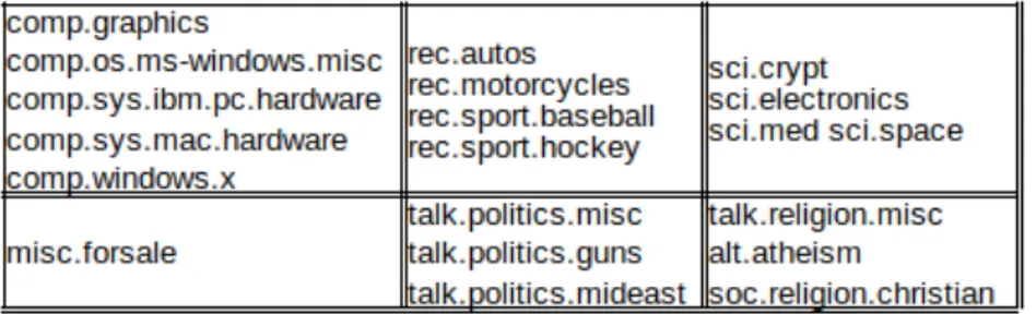
We evaluate the proposed method with two clustered data collections, which are frequently used in the cluster labeling problem. The first collection is 20 News Group (20NG)1 dataset which consists of 20 different topics. There are a total of about 20,000 documents where each category consists of nearly 1,000 documents. The second is the Open Directory Project (ODP) RDF dump2_{. For}

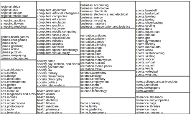
that collection, we only use the snippets from 125 different diverse categories. We randomly chose about 100 documents for each of the clusters, some clusters having less than 100 documents by default, to form the dataset. Topics that are used for experiments are in figures 4.1 and 4.2 for both datasets.

1_{http://people.csail.mit.edu/jrennie/20newsgroups} 2_{http://rdf.dmoz.org/}

Figure 4.1: Clusters of ODP dataset.

4.1.1

Wikipedia Usage

We use Lucene open source search system3 _{to index Wikipedia. We select top}

scored 1,000 articles for all terms in each cluster to run the co-occurrence search for the assessment of contextual relatedness of terms to cluster topics.

4.2

Evaluation Metrics

We follow previous cluster labeling evaluation frameworks [25, 24, 26]. For each cluster, we use the same ground truth labels that are used in [25, 26]. A suggested label is considered as correct if it is identical, an inflection, or a WordNet synonym of the cluster’s correct label [25].

Figure 4.2: Clusters of 20NG dataset.

4.2.1

Match@k

The Match@k measure gives the percentage of clusters that are correctly labeled within k candidate labels. 0 is given to the clusters that have not been labeled in k candidates. An example for Match@k calculation is in Table 4.1.

Table 4.1: Demonstration of Match@k label quality measure calculation. BM25 method finds 8 of the clusters’ labels correctly at k=1. This leads to Match@1 = 8/20 = 0.40. On the other hand, where k=5, BM25 finds 8+2+2+0+1 = 13 of the clusters’ labels correctly which means Match@5 = 13/20 = 0.65.

Rank BM25 BM25 1 8 Match@1 0.40 2 2 Match@2 0.50 3 2 Match@3 0.60 4 0 Match@4 0.60 5 1 Match@5 0.65 6 1 Match@6 0.70 7 0 Match@7 0.70 8 0 Match@8 0.70 9 1 Match@9 0.75 10 0 Match@10 0.75

4.2.2

MRR@k (Mean Reciprocal Rank@k)

candidates. An example for MRR@k calculation is in Table 4.2.

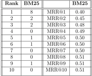
Table 4.2: Demonstration of MRR@k label quality measure calculation. BM25 method finds 8 of the clusters’ labels correctly at k=1. This leads to MRR@1 = (1/1)*8/20 = 0.40. On the other hand, where k=2, MRR@2 for BM25 is ((1/1)*8+(1/2)*2) / 20 = 0.45 which means BM25 finds correct labels for clusters at 2.22nd position on average. Rank BM25 BM25 1 8 MRR@1 0.40 2 2 MRR@2 0.45 3 2 MRR@3 0.48 4 0 MRR@4 0.49 5 1 MRR@5 0.50 6 1 MRR@6 0.50 7 0 MRR@7 0.50 8 0 MRR@8 0.51 9 1 MRR@9 0.51 10 0 MRR@10 0.51

4.2.3

Statistical Test

Statistical tests are used to determine if a result set is statistically significantly different than another result set. We use student’s t-test for evaluating our results against state-of-the-art methods.

The t-test is used to compare two groups of quantitative data with paired ob-servations, Match@k and MRR@k result for our work. It is a convention to first formulate a Null hypothesis which states that there is no effective difference be-tween two groups of results. T-statistic and degrees of freedom are used to decide the correctness of null hypothesis. T-statistic is calculated with the formula:

t = ¯

X1− ¯X2

s_∆¯

and s_∆¯ = s s2 1 n1 + s 2 2 n2 (4.2)

where ¯X1 and ¯X2 are mean values, s1 and s2 are the unbiased estimators of

the variances of two groups.

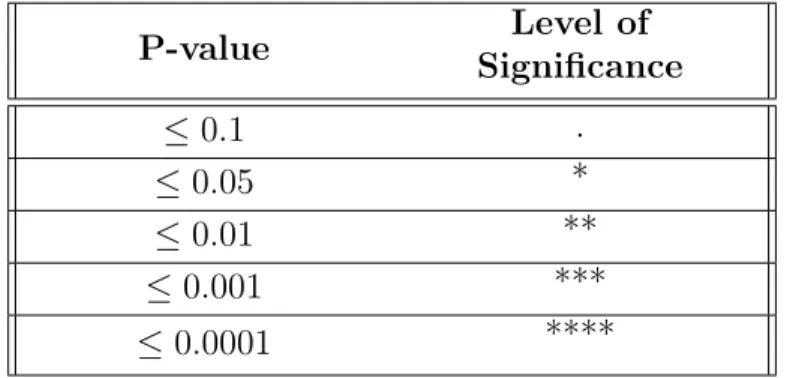
P-values are used to evaluate the outcome of t-tests. The lower p-value is, the stronger the null hypothesis can be rejected which means that two results are significantly different. Levels of significance for difference of two results according to p-value are given in table 4.3.

Table 4.3: Levels of significance for p-values. P-value Level of Significance ≤ 0.1 . ≤ 0.05 * ≤ 0.01 ** ≤ 0.001 *** ≤ 0.0001 ****

Chapter 5

Experimental Results

In this chapter, we present the experimental results for cluster labeling with feature selection methods and contextual relatedness filtering on 20NG and ODP datasets. Previous work focused on Match@k and MRR@k results for up to k=20. We also provide results for up to k=20 but since there will be a limited number of labels that can be provided for clusters, we especially focus on the results that are below k=10 because improvements in that interval are more crucial for labeling quality.

5.1

Feature Selection Methods

We first experiment with the state-of-the-art feature selection methods to see their performance on both datasets.

Figure 5.1 shows the results of feature selection methods on 20NG dataset. MI and JSD methods perform superior to other feature selection methods followed by TF method for both Match@k and MRR@k results. The reason TF method stays below MI and JSD in MRR@k graph is that TF finds correct labels for clusters later than the other two methods. This shows the importance of finding correct labels in higher ranks.

Figure 5.1: MRR@k and Match@k results of feature selection methods on 20NG dataset.

Figure 5.2 shows that JSD and TF methods perform superior to feature selec-tion methods on ODP dataset. The reason MI method perform badly on ODP dataset is due to the usage of only the snippets of documents. [25, 26] gets better results for MI by crawling through the pages to use as ODP dataset.

Figure 5.2: MRR@k and Match@k results of feature selection methods on ODP dataset.

As a result, JSD method performs superior to other methods on both 20NG and ODP datasets as shown in [25]. Thus, we decide to use JSD method along with TF for further experiments on contextual relatedness filtering for their consistent

5.2

Contextual Relatedness Filtering

We evaluate contextual relatedness filtering method on JSD and TF feature se-lection methods with different parameter settings on both datasets.

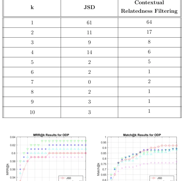
Contextual Relatedness Filtering on JSD . Figure 5.3 and Figure 5.4 show the results of contextual relatedness filtering for JSD method on ODP and 20NG datasets, respectively. As figures demonstrate, contextual relatedness fil-tering significantly improves1 _{the MRR@k results with respect to the baseline}

JSD method for both datasets which means that unrelated terms are successfully filtered out from the candidate label lists, thus relevant terms climb up to be considered as labels at a higher rank. Although JSD passes filtered results in the Match@k graph after k=10 for ODP dataset, it should be remembered that only a few number of terms can be suggested as cluster labels to the users; therefore, terms after k=10, even k=5, does not have practical importance for cluster la-beling problem. The increase in Match@k results before k=10 for both datasets will lead to an increase on the labeling quality which can also be deduced from MRR@k figure.

Figure 5.3: MRR@k and Match@k results of JSD and contextual relatedness filtering on ODP dataset.

Table 5.1 shows an example filtering on ODP dataset for health.pharmacy

Figure 5.4: MRR@k and Match@k results of JSD and contextual relatedness filtering on 20NG dataset.

cluster. The terms ”information, side, usage, full, features and provided” are assessed as unrelated to the topic and removed from the candidate label list. This helps the actual label pharmacy to move from rank 11 to rank 7.

Table 5.2 demonstrates improvements on correct label positions on ODP dataset for k up to 10. Contextual relatedness filtering improves the number of correctly labeled clusters for k < 5 which is the main purpose of our approach for cluster labeling.

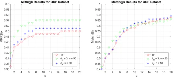
We also experiment with different threshold and n values to see their effects on contextual relatedness assessment. In Figure 5.5, it can be observed that for the low n value, both Match@k and MRR@k results drop low of JSD results. Evaluating related terms unrelated because of the low n value leads to this out-come. Automatic threshold usage improves the results but the performance is still not near the desired level for low n value. Automatic threshold increases the performance because it tunes itself according to each cluster and eliminates some false contextual relatedness assessments.

For 20NG dataset, our JSD results are similar to previous works but our JSD results for ODP dataset are lower. The reason behind this is that we only use snippets of documents rather than crawling through the pages, which feeds the

JSD method with less information about the documents and the clusters.

Table 5.1: A filtering example of contextual relatedness on JSD features. First column is the top 20 terms ranked by JSD scores, second column gives contextual relatedness information of the JSD terms, third column is the new set of JSD terms after removal of contextually unrelated terms.

JSD ranking Relatedness After filtering

effects related effects

information not related prescribing prescribing related dosage

side not related rxlist

dosage related warnings

usage not related drug

rxlist related pharmacy

warnings related precautions full not related patient drug related contraindications pharmacy related indication

features not related pharmacology precautions related consumer

patient related health

contraindications related type

indication related fda

pharmacology related chemical provided not related brand

consumer related names

Table 5.2: Number of clusters that are labeled correctly for k’th label candidates ranked by JSD scores. k JSD Contextual Relatedness Filtering 1 61 64 2 11 17 3 9 8 4 14 6 5 2 5 6 2 1 7 0 2 8 2 1 9 3 1 10 3 1

Figure 5.5: MRR@k and Match@k results of JSD and contextual relatedness filtering on ODP dataset with different threshold and n values.

Contextual Relatedness Filtering on TF . We also apply contextual re-latedness filtering approach on TF feature selection method on ODP dataset to show that it works with more than one feature selection method and the results are not coincidental.

Figure 5.6 shows the results of contextual relatedness filtering for TF method on ODP dataset. As the figure demonstrates, contextual relatedness filtering significantly improves2 _{both the MRR@k and Match@k results with respect to}

the baseline TF method which again means contextual relatedness filtering re-moved unrelated terms from the candidate list, thus relevant terms climb up to be considered as labels at a higher rank.

Figure 5.6: MRR@k and Match@k results of TF and contextual relatedness fil-tering on ODP dataset.

Table 5.3 shows another filtering example on ODP dataset for sports.martial.arts cluster. Several terms that are indeed unrelated to the martial arts are removed from the feature list. This leads to a big bounce for the actual label martial to move from rank 20 to rank 8.

Table 5.4 demonstrates improvements on correct label positions also for TF feature selection method on ODP dataset for k up to 10.

Table 5.3: A filtering example of contextual relatedness on TF features. First column is the top 20 terms ranked by TF scores, second column gives contextual relatedness information of the TF terms, third column is the new set of TF terms after removal of contextually unrelated terms.

TF ranking Relatedness After filtering information not related school

school related karate

includes not related aikido karate related instructor

class not related dojo

schedule not related training

aikido related teaching

instructor related martial contact not related traditional

dojo related arts

training related taekwondo

style not related jitsu

teaching related offering affiliate not related ryu features not related programs

history not related seminars details not related iaido

located not related tai

links not related locations

Table 5.4: Number of clusters that are labeled correctly for k’th label candidates ranked by TF scores. k TF Contextual Relatedness Filtering 1 46 50 2 17 12 3 4 5 4 6 6 5 7 9 6 7 6 7 5 6 8 3 4 9 3 2 10 0 2

P-values for t-tests on TF - contextual relatedness filtering comparison can be found in Table A.3.

Chapter 6

Conclusions and Future Work

In this thesis, we propose a novel approach for contextual relatedness assessment where we determine the contextual relatedness of terms to topics of clusters by counting top-n important terms each important term co-occurred with inside Wikipedia articles. We evaluate terms to be contextually related to topics if im-portant term count of a term’s Wikipedia article is above a threshold. We also proposed the usage of contextual relatedness information for filtering out unre-lated terms from feature lists to enhance feature selection quality. Performance increase in a state-of-the-art internal-cluster labeling method, that selects labels only from the contents of the clusters, demonstrates the contributions of the con-textual relatedness filtering. The concon-textual relatedness filtering approach can also be used for other problem domains such as text classification and clustering, that use feature selection methods, by enhancing the feature quality. Statistical tests on both datasets also show that contextual relatedness filtering approach improve feature selection quality significantly.

As future work, Wikipedia attributes such as links, hyperlinks, anchor texts, titles and categories can be used to extend the candidate labels with the usage of contextual relatedness filtering. In [25, 26], important terms are used as queries to Wikipedia to find relevant Wikipedia categories to the clusters and those cat-egories are added to candidate label pool. Term quality in the queries to feed

to Wikipedia can be improved using contextual relatedness filtering which would lead to improvements of relatedness of Wikipedia pages to the context of the clusters. After Wikipedia suggests new terms to use as labels to clusters, this list of terms can also be filtered with contextual relatedness and this could gain improvement if there can be any.

Bibliography

[1] E. Gabrilovich and S. Markovitch, “Computing semantic relatedness using wikipedia-based explicit semantic analysis,” in Proceedings of the 20th Inter-national Joint Conference on Artifical Intelligence, IJCAI’07, (San Francisco, CA, USA), pp. 1606–1611, Morgan Kaufmann Publishers Inc., 2007.

[2] “Google translate.” https://translate.google.com/intl/en/about/.

[3] “Carrot search engine.” http://search.carrot2.org.

[4] A. L. Blum and P. Langley, “Selection of relevant features and examples in machine learning,” Artif. Intell., vol. 97, pp. 245–271, Dec. 1997.

[5] G. Forman, “An extensive empirical study of feature selection metrics for text classification,” J. Mach. Learn. Res., vol. 3, pp. 1289–1305, Mar. 2003.

[6] A. Dasgupta, P. Drineas, B. Harb, V. Josifovski, and M. W. Mahoney, “Fea-ture selection methods for text classification,” in Proceedings of the 13th ACM SIGKDD International Conference on Knowledge Discovery and Data Mining, KDD ’07, (New York, NY, USA), pp. 230–239, ACM, 2007.

[7] C. D. Manning, P. Raghavan, and H. Sch¨utze, Introduction to Information Retrieval. New York, NY, USA: Cambridge University Press, 2008.

[8] S. Patwardhan, S. Banerjee, and T. Pedersen, “Using measures of seman-tic relatedness for word sense disambiguation,” in Proceedings of the 4th International Conference on Computational Linguistics and Intelligent Text Processing, CICLing’03, (Berlin, Heidelberg), pp. 241–257, Springer-Verlag,

[9] A. Budanitsky and G. Hirst, “Evaluating wordnet-based measures of lexical semantic relatedness,” Comput. Linguist., vol. 32, pp. 13–47, Mar. 2006.

[10] N. Nathawitharana, D. Alahakoon, and D. D. Silva, “Using semantic related-ness measures with dynamic self-organizing maps for improved text cluster-ing,” in 2016 International Joint Conference on Neural Networks (IJCNN), pp. 2662–2671, July 2016.

[11] “Placing search in context: The concept revisited,” ACM Trans. Inf. Syst., vol. 20, pp. 116–131, Jan. 2002.

[12] P. D. Turney, “Similarity of semantic relations,” Comput. Linguist., vol. 32, pp. 379–416, Sept. 2006.

[13] D. B. Lenat and R. V. Guha, Building Large Knowledge-Based Systems; Rep-resentation and Inference in the Cyc Project. Boston, MA, USA: Addison-Wesley Longman Publishing Co., Inc., 1st ed., 1989.

[14] “Wikipedia, the free encyclopedia.” https://www.wikipedia.org/.

[15] E. Yeh, D. Ramage, C. D. Manning, E. Agirre, and A. Soroa, “Wikiwalk: Random walks on wikipedia for semantic relatedness,” in Proceedings of the 2009 Workshop on Graph-based Methods for Natural Language Processing, TextGraphs-4, (Stroudsburg, PA, USA), pp. 41–49, Association for Compu-tational Linguistics, 2009.

[16] “Okapi bm25, wikipedia.” https://en.wikipedia.org/wiki/Okapi BM25/.

[17] D. Carmel, E. Yom-Tov, A. Darlow, and D. Pelleg, “What makes a query difficult?,” in Proceedings of the 29th Annual International ACM SIGIR Con-ference on Research and Development in Information Retrieval, SIGIR ’06, (New York, NY, USA), pp. 390–397, ACM, 2006.

[18] S. Osinski and D. Weiss, “A concept-driven algorithm for clustering search results,” IEEE Intelligent Systems, vol. 20, pp. 48–54, May 2005.

[19] A. Turel and F. Can, “A new approach to search result clustering and la-beling,” in Proceedings of the 7th Asia Conference on Information Retrieval

Technology, AIRS’11, (Berlin, Heidelberg), pp. 283–292, Springer-Verlag, 2011.

[20] H. Toda and R. Kataoka, “A clustering method for news articles retrieval sys-tem,” in Special Interest Tracks and Posters of the 14th International Confer-ence on World Wide Web, WWW ’05, (New York, NY, USA), pp. 988–989, ACM, 2005.

[21] D. R. Cutting, D. R. Karger, J. O. Pedersen, and J. W. Tukey, “Scat-ter/gather: A cluster-based approach to browsing large document collec-tions,” in Proceedings of the 15th Annual International ACM SIGIR Con-ference on Research and Development in Information Retrieval, SIGIR ’92, (New York, NY, USA), pp. 318–329, ACM, 1992.

[22] E. Glover, D. M. Pennock, S. Lawrence, and R. Krovetz, “Inferring hierar-chical descriptions,” in Proceedings of the Eleventh International Conference on Information and Knowledge Management, CIKM ’02, (New York, NY, USA), pp. 507–514, ACM, 2002.

[23] D. R. Radev, H. Jing, M. Sty, and D. Tam, “Centroid-based summarization of multiple documents,” Information Processing and Management, vol. 40, no. 6, pp. 919 – 938, 2004.

[24] P. Treeratpituk and J. Callan, “Automatically labeling hierarchical clusters,” in Proceedings of the 2006 International Conference on Digital Government Research, dg.o ’06, pp. 167–176, Digital Government Society of North Amer-ica, 2006.

[25] D. Carmel, H. Roitman, and N. Zwerdling, “Enhancing cluster labeling using wikipedia,” in Proceedings of the 32Nd International ACM SIGIR Confer-ence on Research and Development in Information Retrieval, SIGIR ’09, (New York, NY, USA), pp. 139–146, ACM, 2009.

[26] H. Roitman, S. Hummel, and M. Shmueli-Scheuer, “A fusion approach to cluster labeling,” in Proceedings of the 37th International ACM SIGIR Con-ference on Research &#38; Development in Information Retrieval, SIGIR

[27] O. S. Chin, N. Kulathuramaiyer, and A. W. Yeo, “Automatic discovery of concepts from text,” in Proceedings of the 2006 IEEE/WIC/ACM Interna-tional Conference on Web Intelligence, WI ’06, (Washington, DC, USA), pp. 1046–1049, IEEE Computer Society, 2006.

[28] J. C. K. Cheung and X. Li, “Sequence clustering and labeling for unsuper-vised query intent discovery,” in Proceedings of the Fifth ACM International Conference on Web Search and Data Mining, WSDM ’12, (New York, NY, USA), pp. 383–392, ACM, 2012.

[29] I. Hulpus, C. Hayes, M. Karnstedt, and D. Greene, “Unsupervised graph-based topic labelling using dbpedia,” in Proceedings of the Sixth ACM In-ternational Conference on Web Search and Data Mining, WSDM ’13, (New York, NY, USA), pp. 465–474, ACM, 2013.

[30] M. Lesk, “Automatic sense disambiguation using machine readable dictio-naries: How to tell a pine cone from an ice cream cone,” in Proceedings of the 5th Annual International Conference on Systems Documentation, SIGDOC ’86, (New York, NY, USA), pp. 24–26, ACM, 1986.

[31] S. Banerjee and T. Pedersen, “An adapted lesk algorithm for word sense disambiguation using wordnet,” in Proceedings of the Third International Conference on Computational Linguistics and Intelligent Text Processing, CICLing ’02, (London, UK, UK), pp. 136–145, Springer-Verlag, 2002.

[32] M. Strube and S. P. Ponzetto, “Wikirelate! computing semantic relatedness using wikipedia,” in Proceedings of the 21st National Conference on Artificial Intelligence - Volume 2, AAAI’06, pp. 1419–1424, AAAI Press, 2006.

[33] S. Jabeen, X. Gao, and P. Andreae, “Harnessing wikipedia semantics for computing contextual relatedness,” in Proceedings of the 12th Pacific Rim International Conference on Trends in Artificial Intelligence, PRICAI’12, (Berlin, Heidelberg), pp. 861–865, Springer-Verlag, 2012.

[34] J. J. Jiang and D. W. Conrath, “Semantic similarity based on corpus statis-tics and lexical taxonomy,” CoRR, vol. cmp-lg/9709008, 1997.

Appendix A

Student’s t-test Results

Table A.1: Statistical tests between JSD and contextual relatedness filtering on 20NG dataset.

Quality Measure Method 1 Method 2 p-value MRR@k JSD Contextual Relatedness Filtering

Manual Threshold(****)

2.56017E-14

MRR@k JSD Contextual Relatedness Automatic Threshold(.)

0.082813843

Match@k JSD Contextual Relatedness Filtering Manual Threshold(***)

0.000119275

Match@k JSD Contextual Relatedness Automatic Threshold(*)

Table A.2: Statistical tests between JSD and contextual relatedness filtering on ODP dataset.

Quality Measure Method 1 Method 2 p-value MRR@k JSD Contextual Relatedness Filtering

Manual Threshold(****)

4.58677E-07

MRR@k JSD Contextual Relatedness Automatic Threshold(-)

0.167850656

Match@k JSD Contextual Relatedness Filtering Manual Threshold(*)

0.012992786

Match@k JSD Contextual Relatedness Automatic Threshold(-)

Table A.3: Statistical tests between TF and contextual relatedness filtering on ODP dataset.

Quality Measure Method 1 Method 2 p-value MRR@k TF Contextual Relatedness Filtering

Manual Threshold(****)

3.98261E-19

MRR@k TF Contextual Relatedness Automatic Threshold(****)

2.73836E-10

Match@k TF Contextual Relatedness Filtering Manual Threshold(*)

0.0377085

Match@k TF Contextual Relatedness Automatic Threshold(****)