Published by Canadian Center of Science and Education
Measuring the Financial Risk Level in Emerging and Developed
Markets: Traditional and Alternative Methods
Samet Günay1
1 Finance, Department of Banking and Finance, School of Applied Sciences, Istanbul Arel University, Istanbul,
Turkey
Correspondence: Samet Günay, Finance, Department of Banking and Finance, School of Applied Sciences, Istanbul Arel University, Istanbul, Turkey. E-mail: [email protected]
Received: January 1, 2015 Accepted: April 11, 2015 Online Published: June 13, 2015 doi:10.5539/ass.v11n16p25 URL: http://dx.doi.org/10.5539/ass.v11n16p25 Abstract
In this study, we measured the financial risk levels of five emerging and five developed markets’ stock indexes using traditional and alternative models. We used the variance, semi-variance, beta, and downside beta, Gaussian VaR, Historical VaR and Cornish-Fisher VaR as the traditional methods; and took the two parameters of the alpha-stable distributions (alpha and beta) and the excess statistic introduced by Harding and Pagan (2002) as alternative models. According to the findings, traditional and alternative models, except for the beta, downside beta, and the excess statistic, gave consistent results in terms of the risk classification between the emerging and the developed markets. Additionally, all models affirmed that the highest risk exists in the stock index of Turkey, whereas the USA stock market has the lowest risk level among the countries analyzed.
Keywords: financial risk level, emerging markets, developed markets, downside risk Jel No: C14, C22, F30
1. Introduction
Measurement of risk is as crucial as at least hedging in finance theory. Financial risk, which can be defined as the deviations of expected return from the realized return, has been measured differently from past to present. Despite extensive literature on this issue, there is still no a consensus regarding the best way of measuring risk. Following the study by Markowitz (1959), who proposed the use of semi-variance as a financial risk measurement tool to assess the risk under a specific target return, this method and its variations have received great interest in literature. In an earlier study, Mao (1970) stated that the return measure of Markowitz is widely accepted, yet there is no consensus regarding risk issue. Indeed, Markowitz proposed five alternative risk measurements besides variance. Mao specifically emphasized semi-variance among these alternatives and argued that investors concern below-mean semi-variance. Hogan and Warren (1972) improved an algorithm known as ES criteria corresponding with the same topic and introduced semi-variance CAPM (ES-CAPM) as an extension of that criteria. Likewise, Klemkosky (1973) demonstrated that semi-standard deviation and mean absolute deviation methods have less bias than the composite measures obtained from CAPM, therefore, he considered them as more robust risk measurement techniques. In a different study, Tse et al. (1993) presented the optimal investment strategy for the investors concerned with the returns that occur below a specific target rate. Turvey and Nayak (2003) proposed a new approximation based on the semi-variance in optimal hedge decisions. The authors calculated the minimum semi-variance hedge rate for the Kansas City wheat and Texas steers. Barndorff-Nielsen et al. (2009), on the other hand, presented a new risk measure named “downside realized semi-variance” considering the high frequency downside movements in asset prices. They asserted that this method is more informative than the standard realized variance statistic.
Bawa and Lindenberg (1977) introduced the Mean-Lower Partial Moment Capital Asset Pricing Model using downside framework and demonstrated that if the probability distribution of portfolio returns displays a normal, stable or student-t distribution, the model reduces to traditional mean-return CAPM. Harlow and Rao (1989) submitted the generalized MLPM and used the mean return of the stock market instead of the risk-free rate as the target return rate. They concluded that target return is implicit in traditional CAPM and explicit in downside risk literature. As for Estrada (2002), he stated that mean semi-variance behavior is a more successful approximation
in risk measurement and demonstrated the efficiency of downside-CAPM compared to the traditional CAPM via the Morgan Stanley Capital Indices database for emerging markets.
Ang et al. (2006) indicated that stock returns require an approximately 6% risk premium per annum, and the reward of the bearing downside risk is not compensated only by the traditional market beta. More recently, Dobrynskaya (2014) introduced the global downside market factor, asserting that it more accurately explains the returns in currency portfolios sorted by the forward discount than the factors discussed in the literature. As aforementioned, downside risk literature generally considers semi-variance as a tool for obtaining optimal hedge ratio and presents different calculation methods. After all, Hwang and Satchell (2000) proposed unobserved fundamental component volatility as an alternative risk measurement tool. This measure can be obtained by using a stochastic volatility model that filters out the signal in volatility information. Similarly, Bertsimas et al. (2004) introduced a new risk measure called shortfall and analyzed its relationship with different methods such as standard deviation, VaR, lower partial moments and coherent risk measure. According to the revealed facts, mean-shortfall approximation has some advantages over mean-variance.
As a prominent market risk measure, the VaR model was first introduced by JP Morgan to define the maximum loss to which a portfolio may be exposed in a crisis such as the market collapse in 1978 and Barings Bank scandal. Many alternative VaR models were presented by different researchers in the following years; most notably Variance Covariance VaR (The delta-normal VAR), Delta-Gamma VaR, Monte Carlo simulation and Historical Simulation and so on. Probability distribution of returns used in the VaR analysis is very important regarding the credibility of results. When the tail structure of the distribution is predicted differently from the actual distribution due to an invalid distribution assumption, VaR can be less than real figures. As stated by Mandelbrot (1963) and Nolan (1997), financial asset returns exhibit fat tail features, hence many authors highlighted the importance of alpha-stable distributions: Fama (1970), Liu et al. (1999), Plerou et al. (1999), Ghahfarokhi and Ghahfarokhi (2009) and Wang et al. (2012). According to Mandelbrot (2004), financial risk had not been measured correctly. He proposed using alpha parameter as a risk measure in finance, a statistic of alpha-stable distributions that characterizes the fluctuation. In line with this suggestion, we calculated the alpha-stable distribution parameters for all the index returns used and considered alpha and beta statistics as an alternative risk measure to traditional methods. In addition, considering the criticisms on normal distribution in literature, we used Cornish-Fisher VaR method in conjunction with Gauissian VaR and Historical VaR. Authors such as Pichler and Selitsch (1999) and Jaschke and Jiang (2002) demonstrated the robustness of this model as a market risk measure.
The last alternative risk measure, the excess statistic introduced by Harding and Pagan (2002), is a test to define the shape of bull and bear markets. This shape also gives information about the risk structure of price movements describing convex and concave shapes in the path of prices. In spite of the fact that this statistic has been used to define the shape of bull and bear markets in different studies such as the ones by Smith and Summers (2002), Camacho et al. (2008), and Ingram (2014), we utilized it as a risk measure.
In this study, financial risk assessment is measured for five emerging markets and five developed markets using different methods. Although risk measurement is generally classified under the titles of market risk, credit risk, and operational risk, in the present study we analyzed traditional risk measurements and alternative methods without using a specific category and investigated their consistency. The main difference between traditional and alternative models is related to their assumptions. Mandelbrot and Hudson (2004) suggested using alpha parameter of stable distributions instead of standard deviation or variance in the measurement of financial risk. Due to the fact that as stated by Taleb (2007), most of the traditional models, such as standard deviation, variance, CAPM beta and parametric VaR, are based on the bell shaped normal distribution that does not take big market movements into account. However we know that the alpha parameter of stable distributions provide a risk information concerning the extreme events measuring tail thickness of the stable distribution, which has thicker tails comparing to normal distribution. Our second alternative risk measure is the excess statistic. In fact, this statistic has been introduced just to analyze the movements of bull and bear periods of financial assets by Harding and Pagan (2002). As we explain in the following sections, these movements can follow sharp or smooth paths depending on the properties of time series. Despite the fact that excess statistic has been utilized to the analyze the shape of bull and bear periods, we consider it as a financial risk indicator since it gives information about the behavior of price series in the period of bull and bear markets and does not depend on the distribution type of returns.
The remaining of the paper is organized as follows: Second section presents the econometrical methodology concerning the methods used in the empirical analysis, third section empirically examines different risk
measurements, traditional and alternative methods. The final section discusses the findings and presents the results.
2. Methodology
2.1 Downside Risk Measures
In a rising market, any asset with downward movements is not attractive for investors and therefore such assets expose higher rate of risk premium requirement in the market (Ang et al., 2006). Considering this information one of the two important downside risk measures, downside beta, can be calculated for assets and as
shown below. Asset has three possible payoffs: , and ; similarly asset has two possible payoffs:
and . These payoffs are above the risk free interest rate and possibilities of them are as follows: Table 1. Payoffs and probabilities
payoff probability ( , ) ( , ) ( , ) ( , ) ( , ) ( , )
For an investor, the optimal portfolio weights are calculated with the statement below: max
, 1
where demonstrates the weight of asset in the portfolio, and the portfolio value at the end of
period is as below:
2
where is gross risk free interest rate. For this example, downside beta can be identified as follows:
cov , |
var | 3
where is the excess return of asset (market) and is a mean market excess return (Ang et al., 2006).
As for semi-variance, it is defined as below:
,0 4
where is the expectation operator, is the random returns variable and is the reference point. can also be an expected value or targeted return rate. Thus, semi-variance is measured as expected value of squared returns under a certain targeted return rate (Turvey & Nayak, 2003).
2.2 VaR Models
VaR provides data for the investor concerning the highest losses to which the portfolio value can be exposed at a specific confidence level and time interval. This information gives investor confidence and allows them to be prepared for potential losses. As the probability distributions are used in the calculation of VaR, VaR value presents the maximum loss within a probability level. As it can be seen, preferred distribution type and its tail structure are very significant for the quantity and credibility of VaR results. Cornish-Fisher model, one of the alternative VaR methods, would be preferred when the returns display a non-Gaussian distribution. This method considers the high moments in the probability distribution, hence the fat tails in the return distribution are taken into account in the model. Under the assumption that log-returns of a portfolio are normally distributed, classical VaR is calculated as follows:
VaR 5
Where is the critical value at confidence level for parametric VaR. Under the same assumption
CFVaR 6 1 6 3 24 2 5 36 7
Where S(X) and K(X) are skewness and kurtosis parameters and denotes the Cornish-Fisher critical value at
confidence interval . When returns follow a normal distribution, classical VaR and Cornish-Fisher VaR values will be equal. However, if the return distribution of portfolio strays moderately from the normal the Cornish-Fisher VaR will be more credible. For serious deviations from the normal distribution, different models must be used (Aktaş & Sjöstrand, 2011).
2.3 Parameters of Alpha-stable Distribution
From a statistical perspective, risk profile for any financial asset can be analyzed using the probability distribution of potential returns of the asset. This distribution involves all the uncertainty of returns and the magnitude of potential risk exposure (Lobato et al., 2007). Therefore, the statistical properties of the return distribution present critical information concerning the risk level of a financial asset. As stated by Mandelbrot (1963), financial asset returns display serious deviations from the normal distribution and present fat tails decayed with a power law. Under these conditions, Mandelbrot suggested using alpha-stable distributions in financial modeling. Han (2010) demonstrated that one-dimensional stable distributions can be defined uniquely by their characteristic functions.
exp | | 1 sign tan
2 , if α 1
exp | | 1 2sign log
2 , if α 1
8
Where sign is the sign of . In the definition of alpha-stable distributions, four parameters are used:
, , and . The first two of these parameters, alpha and beta, are useful as a financial risk indicator as
suggested by Mandelbrot. The α (0 2) determines the tail thickness of the distribution. The ( ∞
∞) is the location parameter, for 1 2 and 0 1, corresponding to mean and variance,
respectively. The is the scale parameter ( 0) and demonstrates the dispersion around the location
parameter, hence it is analogous standard deviation. As for , it is symmetry parameter ( 1 1) and
which defines the skewness of the distribution. The distribution is symmetrical when 0, skewed to right for
0 and skewed to left for 0 (Han et al., 2010).
2.4 Excess Statistic
Harding and Pagan (2002) introduced an algorithm which produces four statistics, in order to define business cycles of bull and bear markets. One of these statistics is the excess statistic that defines the shape of phases. If the transition between two successive turning points is linear, this statistic measures the magnitude of deviations from a hypothetical path of the actual time series’ path. That is, excess statistic is an intuitive approximation concerning the second derivative of the series and informs about the convexity or concavity of the series (Camacho et al., 2008). Therefore, obtained value of excess statistic presents the characteristic of the phases of bull and bear markets and identifies the risk of price movements. Calculation process of the excess statistic can be explained via the following definition utilizing other statistics of Harding and Pagan (2002): average duration of each phase is D, average magnitude of each phase is A, and average cumulative movement in over each phase is C (Note 1). In that situation, the shape of each phase can be measured as the deviations from a triangle. Using this definition excess statistic:
2 2 9
Following the assumption, binary-dual random variable will be equal to 1 for bull periods and 0 for bear period, the process of obtaining the parameters of excess statistic is explained as follows: In an expansion, total
elapsed time is ∑ and the number of the peaks is ∑ 1 . Average elapsed time in an
expansion is
10 and the average magnitude of expansions is
∆ln 11 As for the mean of total cumulative changes, it is
12
where ∆ln and 0 (Pagan & Sossounov, 2003).
3. Empirical Analysis
In this section of the study, obtained results of the econometric modeling will be discussed. Firstly, we estimate the values of traditional risk measures: variance, semi-variance, beta, downside beta, Gaussian VaR, Historical VaR and Cornish-Fisher VaR, and secondly alternative models, alpha and beta parameters of the alpha-stable distribution and excess statistics of Hardin and Pagan (2002), are estimated for each index. Finally, we compare the order of the risk volume of each model. Using the classification of Morgan Stanley Capital International (henceforth MSCI) we determined five emerging and five developed stock markets as follows: Bist 100 (Turkey), Bovespa (Brazil), Rts (Russia), Sensex (India), Shanghai (China), DJIA (USA), Nikkei225 (Japan), Ftse 250 (England), Dax (Germany), Cac-40 (France). Sample interval of the study consists of the period of between February 05, 2004 and July 01, 2014. Except for the excess statistic, which was obtained with price series, all of the statistics are calculated using log-returns. Variance, semi-variance, beta, downside beta, and VaR tests are conducted through the R code of Carl and Peterson (2014). Alpha and beta parameter estimations of alternative models are performed using the Matlab code of Weron (2006). Excess statistics are calculated with the Gauss code of Engel (2005). All of the index values were obtained from finance.yahoo.com.
3.1 Traditional Methods
3.1.1 Downside Models and VaR
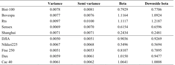
In Table 2 below, we present variance, semi-variance, beta and downside beta statistics of developed and emerging market stock index log-returns. Semi-variance measures the volatility of negative returns unlike traditional variance method. The variance statistics demonstrate that the results support our discrimination between the emerging and the developed markets. While there is a clustering among the emerging markets such as India, Brazil, China, Turkey and Russia, the developed markets of England, France, USA, Germany, Japan, are seen in a second group. Semi-variance results are also consistent with the orders of variance, that is, the discrimination between the emerging and the developed markets is very clear in terms of variance and semi-variance statistics of log-returns. This situation can be seen as a risk difference of two groups of economies. Findings indicate that the riskiest stock markets are the Turkish and Russian stock markets, whereas the lowest risks are seen in the USA and UK.
The second comparison is made for the beta and the downside beta statistics in all stock index returns. Beta is a systematic risk measure and it quantifies the changing level of systematic risk of a well-diversified portfolio after adding a new asset to the portfolio. Technically, beta gives the slope coefficient of the regressing market returns and a specific stock returns. Hence, beta is an efficient measure for examining the sensitivity of stock returns to the changing market returns. As for the downside beta, it measures the same sensitivity of the negative returns. Higher values of beta are considered as an indication of higher levels of systematic risk. For instance, two stocks with two different beta values, 0.5 and 2, indicate two different situations. The first one only moves half as much as the market linearly, whereas the second one does the same movement twofold. For the calculation of beta and downside beta, we use The MSCI World Index as market portfolio. Findings indicated that the clustering and the order of the developed and emerging market stock index log-returns changed significantly for the beta and the downside beta statistics. While the beta and downside beta of USA, Germany and France stock indexes are close to market beta 1, China stock market has the lowest rate of interaction with the global stock market. According to both beta and downside beta values (0.2434 and 0.2481 respectively), China stock market changes at the rate of 25% of global stock market in its fluctuations. The Russian and Brazilian stock markets, on the other hand, are more sensitive to global stock market movements. The highest value of downside beta (1.2187) belongs to the Russian stock market implying that a unit change in the negative returns of global stock market causes a variation of 1.22 in the negative returns of Russian stock index RTS.
Table 2. Traditional risk measures (a)
Variance Semi variance Beta Downside beta
Bist-100 0.0078 0.0081 0.7929 0.7706 Bovespa 0.0077 0.0076 1.1164 1.0924 Rts 0.0097 0.0100 1.1117 1.2187 Sensex 0.0069 0.0070 0.6154 0.6596 Shanghai 0.0071 0.0071 0.2434 0.2481 DJIA 0.0050 0.0051 0.9036 0.9269 Nikkei225 0.0067 0.0068 0.5496 0.5694 Ftse 250 0.0051 0.0053 0.8107 0.7895 Dax 0.0059 0.0061 1.0150 0.9477 Cac 40 0.0061 0.0062 1.0641 1.0008
Table 3 below exhibits the results of Gaussian VaR, Historical VaR and Cornish-Fisher VaR models at 95% confidence level for one day. Gaussian VaR assumes the normality of probability distribution of returns. Historical VaR assumes that the probability distribution of existing data is valid in the current situation. Cornish-Fisher method considers the factors that normal distribution does not take into account such as skewness and kurtosis. As known, probability distribution of financial asset returns displays fat tails and asymmetry properties. Cornish-Fisher VaR model can yield more efficient estimates considering these facts.
Table 3. Traditional risk measures (b)
Gaussian VaR Historical VaR Cornish-Fisher VaR
Bist-100 -0.0125 -0.0126 -0.0126 Bovespa -0.0125 -0.0124 -0.0113 Rts -0.0158 -0.0145 -0.0118 Sensex -0.0111 -0.0104 -0.0100 Shanghai -0.0116 -0.0115 -0.0111 DJIA -0.0081 -0.0072 -0.0071 Nikkei225 -0.0111 -0.0101 -0.0096 Ftse 250 -0.0082 -0.0085 -0.0079 Dax -0.0096 -0.0089 -0.0087 Cac 40 -0.0101 -0.0094 -0.0091
As seen in Table 3, the results of all three models are consistent internally and with the findings of variance and semi-variance models.
Bist 100 Bovespa
Rts Sensex
Shanghai DJIA
Nikkei 225 Ftse 350
Dax Cac 40
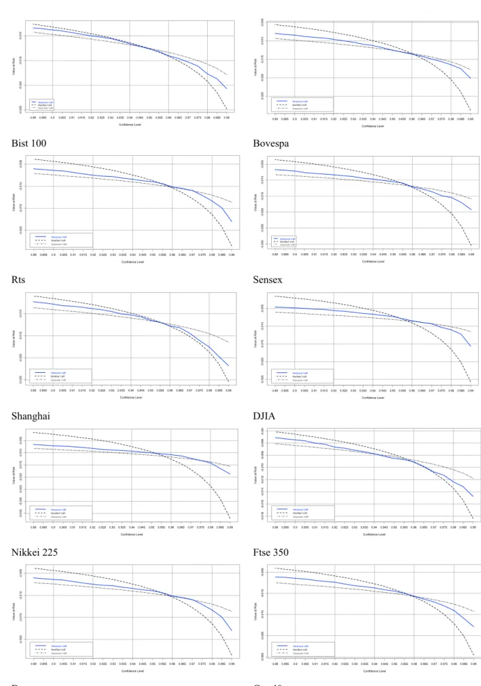
Figure 1. Risk confidence sensitivity of VaR methods
0.890.895 0.9 0.905 0.910.9150.920.9250.93 0.9350.940.9450.950.955 0.960.9650.970.9750.98 0.9850.99 Confidence Level -0 .025 -0 .020 -0 .0 15 -0 .010 Historical VaR Modified VaR Gaussian VaR V a lu e at R is k 0.890.895 0.90.905 0.91 0.9150.920.9250.93 0.9350.940.9450.950.955 0.960.965 0.970.9750.980.9850.99 Confidence Level -0 .025 -0 .020 -0 .015 -0 .010 -0 .005 Historical VaR Modified VaR Gaussian VaR Val u e a t R is k 0.89 0.8950.9 0.905 0.91 0.9150.920.9250.93 0.9350.940.9450.950.955 0.960.9650.970.9750.98 0.9850.99 Confidence Level -0 .0 20 -0 .0 1 5 -0 .0 1 0 -0 .0 05 Historical VaR Modified VaR Gaussian VaR Va lu e a t R is k 0.890.895 0.9 0.905 0.910.9150.920.925 0.93 0.9350.940.9450.950.955 0.960.9650.97 0.9750.98 0.9850.99 Confidence Level -0 .030 -0 .025 -0 .0 20 -0 .0 1 5 -0 .0 1 0 -0 .005 Historical VaR Modified VaR Gaussian VaR V al ue at R is k 0.890.8950.9 0.905 0.910.9150.920.925 0.93 0.9350.940.9450.950.955 0.960.9650.970.9750.98 0.9850.99 Confidence Level -0 .025 -0 .020 -0 .0 15 -0 .010 Historical VaR Modified VaR Gaussian VaR V a lue at R is k 0.890.895 0.9 0.905 0.910.9150.920.9250.93 0.9350.940.9450.950.955 0.960.9650.970.9750.98 0.9850.99 Confidence Level -0 .0 2 5 -0 .020 -0 .015 -0 .0 1 0 -0 .005 Historical VaR Modified VaR Gaussian VaR Val u e a t R is k 0.890.895 0.9 0.905 0.910.9150.920.925 0.93 0.9350.940.9450.950.9550.960.9650.970.9750.98 0.9850.99 Confidence Level -0 .0 3 5 -0 .030 -0 .025 -0 .020 -0 .015 -0 .010 -0 .005 Historical VaR Modified VaR Gaussian VaR V al ue at R is k 0.89 0.8950.9 0.905 0.91 0.9150.920.9250.930.9350.940.9450.950.955 0.960.9650.970.9750.98 0.9850.99 Confidence Level -0 .0 18 -0 .0 1 6 -0 .0 1 4 -0 .0 12 -0 .0 10 -0 .0 08 -0 .0 0 6 -0 .0 0 4 Historical VaR Modified VaR Gaussian VaR Va lu e a t R is k 0.89 0.8950.9 0.905 0.91 0.9150.920.9250.93 0.9350.940.9450.950.955 0.960.9650.970.9750.98 0.9850.99 Confidence Level -0 .0 20 -0 .0 1 5 -0 .0 1 0 -0 .0 05 Historical VaR Modified VaR Gaussian VaR Va lu e a t R is k 0.890.895 0.90.905 0.910.9150.92 0.9250.930.9350.94 0.9450.950.955 0.960.9650.970.9750.980.9850.99 Confidence Level -0 .0 2 5 -0 .0 20 -0 .0 1 5 -0 .0 10 -0 .0 0 5 Historical VaR Modified VaR Gaussian VaR Val ue a t R isk
Reconsidering these results, the risk differences between emerging and developed markets are seen clearly in the market risk measure VaR models. Besides, the emerging markets have higher level of market risk than the developed markets, for instance Turkey, Russia and Brazil catch attention in terms of the level of market risk. Another interesting finding is the changing risk order depending on the skewness and kurtosis of the probability distribution. While the riskiest stock market is RTS in the Gaussian VaR and Historical VaR model, we see that the risk order changes and the Turkish stock market shifts to first in the order, considering the third and fourth moments of the distribution.
The plots in Figure 1 demonstrate the risk confidence sensitivity concerning all three methods for each country. The horizontal axis presents the confidence level, and the vertical axis indicates VaR value against the change in confidence level. Note that in conjunction with the increments in the confidence level, the largest falls occur in the Gaussian VaR model. Pursuant to our statistical expectations for the lower confidence levels, we obtained higher VaR values in all models.
3.2 Alternative Methods
3.2.1 Two Parameters of Alpha-stable Distributions: Alpha and Beta
The second section of the empirical analysis presents the alpha and beta parameter values of the alpha-stable distributions of all stock index returns. It is known that normal distribution displays thinner tails than the actual case in financial markets and reduces the probabilities of extreme events to insignificant levels.
As stated by Mandelbrot (1963), Fama (1970) and Peters (1994), alpha-stable distributions can fit the data
without any need for corrections. The first parameter of the distribution α (0 2) demonstrates the tail
thickness of the distribution, that is, the risk of the returns. is the symmetry parameter of the distribution and
it defines the skewness. The distribution is symmetric for 0, skewed to the right for 0, and skewed
to the left for 0 (Han et al., 2010). As the tail thickness parameter is related to the probability of extreme
events, it is a highly significant risk measure. Taleb (2007) dedicated his entire book The Black Swan: The Impact of the Highly Improbable to this fact.
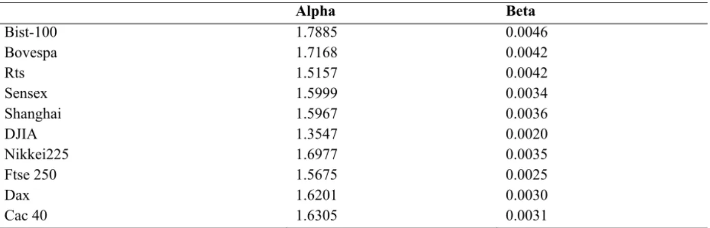
Table 4. Alternative risk measures (a)
Alpha Beta Bist-100 1.7885 0.0046 Bovespa 1.7168 0.0042 Rts 1.5157 0.0042 Sensex 1.5999 0.0034 Shanghai 1.5967 0.0036 DJIA 1.3547 0.0020 Nikkei225 1.6977 0.0035 Ftse 250 1.5675 0.0025 Dax 1.6201 0.0030 Cac 40 1.6305 0.0031
According to the alpha results in Table 4, the thickest and the thinnest tails belong to the stock index of Turkey and the USA, respectively, implying that the most extreme events are seen in Turkish stock market among the markets examined. Distinct from the previous results, there is an interesting order for the remaining indexes. Regarding the tail thickness parameter alpha, risk concentration in the markets of Russia, China and India appears smaller than those of Germany, France and Japan. More clearly, frequency rate of the extreme events in Germany, France and Japan is higher than Russia, China and India stock markets. Risk concentration in Brazil’s stock market, meanwhile, is the closest value to the Turkish stock market. Findings concerning the beta statistic exhibited the same order results as alpha. According to beta values, all countries’ return distributions are skewed towards to the right, meaning, prone to low returns. This finding is commonly accepted for the stock market returns and in accordance with our expectations the highest beta (skewness) values are seen in the returns of Brazil, Russia and Turkey, and the lowest beta value belongs to the USA stock market. These results are consistent with the findings of the previous tests; variance, semi-variance, VaR, alpha and beta parameters of alpha-stable distribution.
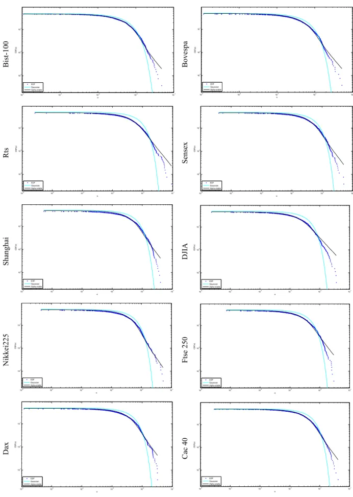
Bist-100 B oves pa Rts Sense x Sha nghai DJI A N ikk ei22 5 Ftse 250 Dax Cac 40
Figure 2. Stable, gaussian, and empirical left tails 10-5 10-4 10-3 10-2 10-1 10-3 10-2 10-1 -x CDF (x ) EDF Gaussian Alpha-stable 10-5 10-4 10-3 10-2 10-1 10-3 10-2 10-1 -x CDF (x ) EDF Gaussian Alpha-stable 10-6 10-5 10-4 10-3 10-2 10-1 10-3 10-2 10-1 -x CD F (x ) EDF Gaussian Alpha-stable 10-6 10-5 10-4 10-3 10-2 10-1 10-3 10-2 10-1 -x CDF (x ) EDF Gaussian Alpha-stable 10-6 10-5 10-4 10-3 10-2 10-1 10-3 10-2 10-1 -x CDF (x ) EDF Gaussian Alpha-stable 10-6 10-5 10-4 10-3 10-2 10-1 10-3 10-2 10-1 -x CD F (x ) EDF Gaussian Alpha-stable 10-6 10-5 10-4 10-3 10-2 10-1 10-3 10-2 10-1 -x CD F (x ) EDF Gaussian Alpha-stable 10-6 10-5 10-4 10-3 10-2 10-1 10-3 10-2 10-1 -x CD F (x ) EDF Gaussian Alpha-stable 10-6 10-5 10-4 10-3 10-2 10-1 10-3 10-2 10-1 -x CDF (x ) EDF Gaussian Alpha-stable 10-6 10-5 10-4 10-3 10-2 10-1 10-3 10-2 10-1 -x CD F (x ) EDF Gaussian Alpha-stable
The plots index retur alpha-stab validity of 3.2.2 Exce The excess provides v In this sen in Figure bull and be Co Co Figure 3 p the excess (negative) exhibits gr concave e When the 2008). As can be behavior in of recessio bear phase and transit behavior. A period in C opposite b in Figure 2 de rns and represe le distribution f the previous o ess Statistic s statistic intro valuable inform nse, excess stat 3 exhibits the ear markets. onvex Expansi onvex Recessi Figure 3 presents signif s statistic. Con excess statist radual change xpansion and excess statisti seen from the n bear periods on periods in T es. Conversely t to bull phase All of the inde China stock ind behavior.
emonstrate the ent a magnific ns fit the empi observations re oduced by Hard mation regardin tistic gives inf
possible mov ion (Excess>0 ion (Excess>0) 3. Stable, gauss ficant informat nvex (concave tic. Despite th s in the beginn convex recess ic is equal to z e excess statist s, whereas all o Turkey, stock i y, bear periods s. The most st exes have posi dex starts to in
e right tail of e cation of the rig
irical data bett egarding the al ding and Paga ng the steepne formation abou vements of the
0)
)
sian, and empi tion about the e) actual paths
he fact that th ning of the ph sion, the actua zero, the move tics in Table 5 other countrie ndex returns f s of other inde triking results itive excess sta ncrease rapidly
empirical, norm ght tail fit on a ter than the no lpha-stable dis an (2002) to de ss of the move ut the risk stru e time series in
irical left tails relationship b are character he actual path hase, these mo al path starts w ement of the s below, stock s exhibit conc fall sharply and
x returns disp are seen in the atistic, wherea y and over slow
mal and alpha-a double logalpha-ari ormal distribut stribution. efine the charac ements of a tim ucture of the ti n accordance w Concave Expa Concave Rece (Source: Cama between the sh rized by positi h in convex ex ovements exten with steep cha series in both p
index returns ave movemen d the movemen
lay slow falls e China stock as China has ne wly while the o
-stable distribu ithmic scale. A tion. This resu
cteristics of bu me series follow
imes series’ be with the exces
ansion (Excess ession (Excess acho et al., 200 hape of the cy ive (negative) xpansion and nd at the end. anges and grad
phases is linea of Turkey dem nts implying th nts are more gr at the start an index regardin egative value. other countries
utions for all o As seen in Figu ult also verifie
ull and bear pe wing turning p ehaviors. The ss statistic valu s<0) <0) 08)
cle and the sig slope and pos concave rece Conversely, in dually flattens ar (Camacho e monstrate a co hat in the begin radual at the en nd end quite sl
ng the bull per It implies that s’ indexes show of the ure 2, es the riods points. plots ue in gn of sitive ssion n the s out. et al., onvex nning nd of owly riod’s t bull w the
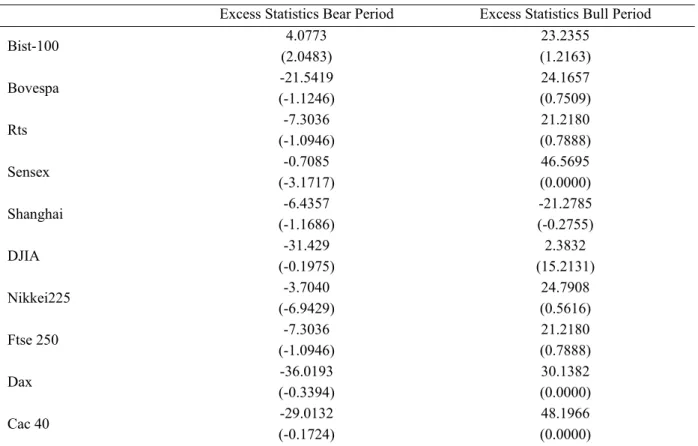
Table 5. Alternative risk measures (b)
Excess Statistics Bear Period Excess Statistics Bull Period
Bist-100 4.0773 (2.0483) 23.2355 (1.2163) Bovespa -21.5419 (-1.1246) 24.1657 (0.7509) Rts -7.3036 (-1.0946) 21.2180 (0.7888) Sensex -0.7085 (-3.1717) 46.5695 (0.0000) Shanghai -6.4357 (-1.1686) -21.2785 (-0.2755) DJIA -31.429 (-0.1975) 2.3832 (15.2131) Nikkei225 -3.7040 (-6.9429) 24.7908 (0.5616) Ftse 250 -7.3036 (-1.0946) 21.2180 (0.7888) Dax -36.0193 (-0.3394) 30.1382 (0.0000) Cac 40 -29.0132 (-0.1724) 48.1966 (0.0000)
Analyzing the findings of bull and bear periods jointly we see that there are two stock indexes deviating from the general trend: those of Turkey and China. After all, if we consider the bear periods in terms of the downside risk, we can say that the sharpest falls are observed in the Turkish stock index BIST, and the riskiest stock market regarding the excess statistic is the Turkish stock market among the emerging and developed markets.
4. Conclusion
Risk is an inseparable part of financial modeling and financial markets. Although there is extant literature regarding the risk measurement under different approaches, there is no consensus about the performance of these risk measurement methods. In this study, without broaching the subject of method performance, we analyzed the financial risk levels of the markets in emerging and developed countries using stock indexes data. In this context, we examined the stock index’s risk levels of five emerging (Turkey, Brazil, Russia, India and China) and five developed countries (USA, UK, Germany, France and Japan) using traditional and alternative methods. The results of traditional (variance, semi-variance, beta, downside beta, Gaussian VaR, Historical VaR, Corinish-Fisher VaR) and alternative models (Excess statistic of Harding and Pagan (2002), alpha and beta parameters of alpha-stable distributions) both confirmed that all these countries nearly consist of two different groups of financial risk similar to the classification of the MSCI. After all, we observed that beta, semi-beta and excess statistic generated different risk level orders which did not allow us to discriminate emerging and developed markets in terms of risk of stock index returns.
References
Aktaş, Ö., & Sjöstrand, M. (2011). Cornish-Fisher Expansion and Value-at-Risk method in application to risk management of large portfolios. Technical report, IDE1112, 1-94.
Ang, A., Chen, J., & Xing, Y. (2006). Downside Risk. Review of Financial Studies, 19(4), 1191-1239. http://dx.doi.org/10.1093/rfs/hhj035
Barndorff-Nielsen, O. E., Kinnebrock, S., & Shephard, N. (2009). Measuring downside risk: Realized semivariance. In T. Bollerslev, J. Russell, & M. Watson (Eds.), Volatility and Time Series Econometrics: Essays in Honor of Robert F. Engle (pp. 117-136). Oxford University Press.
Bawa, V., & Lindenberg, E. (1977). Capital market equilibrium in a mean lower partial moment framework. Journal of Financial Economics, 5, 189-200. http://dx.doi.org/10.1016/0304-405X(77)90017-4
Bertsimas, D., Lauprete, G. R. J., & Samarov, A. (2004). Shortfall as a risk measure: Properties, optimization and applications. Journal of Economic Dynamics & Control, 28, 1353-1381. http://dx.doi.org/10.1016/S0165- 1889(03)00109-X
Camacho, M., Perez-Quiros, G., & Saiz, L. (2008). Do European business cycles look like one? Journal of Economic Dynamics and Control, 32(7), 2165-2190. http://dx.doi.org/10.1016/j.jedc.2007.09.018
Carl, P., & Peterson, B. G. (2014). Package ‘Performance Analytics’. Retrieved from http://r-forge.r-project. org/projects/returnanalytics/
Dobrynskaya, V. (2014). Downside Market Risk of Carry Trades. Review of Finance, 18(5), 1885-1913. http://dx.doi.org/10.1093/rof/rfu004
Engel, J. (2005). James Engel's Business Cycle Dating Matlab Programs. National Centre for Econometric Research. Retrieved from http://www.ncer.edu.au/data/data.jsp
Estrada, J. (2002). Systematic risk in emerging markets: The D-CAPM. Emerging Markets Review, 365-379. http://dx.doi.org/10.1016/S1566-0141(02)00042-0
Fama, E. F. (1970). Efficient Capital Markets: A Review of Empirical Work. Journal of Finance, 25(2), 383-417. http://dx.doi.org/10.2307/2325486
Ghahfarokhi, M. A. B., & Ghahfarokhi, P. B. (2009). Applications of Stable Distributions in Time series analysis, Computer sciences and financial markets. World Academy of Science, Engineering and Technology, 3, 862-864.
Han, D., Tsung, F., Li, Y., & Xian, J. (2010). Detection of changes in a random financial sequence with a stable distribution. Journal of Applied Statistics, 37(7), 1089-1111. http://dx.doi.org/10.1080/02664760902914433 Harding, D., & Pagan, A. (2002). Dissecting the cycle: A methodological investigation. Journal of Monetary
Economics, 49, 365-381. http://dx.doi.org/10.1016/S0304-3932(01)00108-8
Harlow, W. V., & Rao, R. K. S. (1989). Asset pricing in a generalized mean-lower partial moment framework: Theory and evidence. Journal of Financial and Quantitative Analysis, 24(3), 285-311. http://dx.doi.org/10. 2307/2330813
Hogan, W. W., & Warren, J. M. (1972). Computation of the Efficient Boundary in the E-S Portfolio Selection Model. Journal of Financial and Quantitative Analysis, 7(4), 1881-1896. http://dx.doi.org/10.2307/2329623 Hwang, S., & Satchell, S. (2000). Market risk and the concept of fundamental volatility: Measuring volatility
across asset and derivative markets and testing for the impacts of derivatives markets on financial markets. Journal of Banking and Finance, 24, 759-785. http://dx.doi.org/10.1016/S0378-4266(99)00065-5
Ingram, S. R. (2014). Commodity Price Changes are Concentrated at the End of the Cycle. Retrieved from http://www.business.uwa.edu.au/__data/assets/pdf_file/0005/2585201/14-20-Commodity-Price-Changes-ar e-Concentrated-at-the-End-of-the-Cycle.pdf
Jaschke, S., & Jiang, Y. (2002). Approximating Value at Risk in Conditional Gaussian Models. Applied quantitative finance, 3-33. http://dx.doi.org/10.1007/978-3-662-05021-7_1
Klemkosky, R. C. (1973). The Bias in Composite Performance Measures. Journal of Financial and Quantitative Analysis, 8(3), 505-514. http://dx.doi.org/10.2307/2329649
Liu, Y., Gopikrishnan, P., Cizeau, P., Meyer, M., Peng, C. K., & Stanley, H. E. (1999). Statistical properties of the volatility of price fluctuations. Physical Review E, 60(2), 1390-1400. http://dx.doi.org/10.1103/PhysRevE. 60.1390
Lobato, J. M. H., Lobato, D. H., & Suarez, A. (2007). Time Series Models for Measuring Market Risk. Universidad Autonoma de Madrid, Technical Report, 1-57.
Mandelbrot, B. B. (1963). The variation of certain speculative prices. Journal of Business, 36, 392-417. http://dx.doi.org/10.1086/294632
Mandelbrot, B. B., & Hudson, R. L. (2004). The (Mis)behaviour of Markets: A Fractal View of Risk, Ruin, and Reward. London: Profile Books.
Mao, J. C. T. (1970). Models Of Capital Budgeting, E-V Vs. E-S. Journal of Financial and Quantitative Analysis, 5(5), 657-676. http://dx.doi.org/10.2307/2330119
Nolan, J. P. (1997). Numerical calculation of stable densities and distribution functions. Stochastic Models, 13(4), 759-774. http://dx.doi.org/10.1080/15326349708807450
Pagan, A. R., & Sossounov, K. A. (2003). A simple framework for analysing bull and bear markets. Journal of Applied Econometrics, 18(1), 23-46. http://dx.doi.org/10.1002/jae.664
Peters, E. E. (1994). Fractal Market Analysis: Applying Chaos Theory to Investment and Economics. USA: John Wiley & Sons.
Pichler, S., & Selitsch, K., (1999). A comparison of analytical VaR methodologies for portfolios that include options. Retrieved from http://www.tuwien.ac.at/E330/Research/paper_var.pdf.WorkingPaperTUWien Plerou, V., Gopikrishnan, P., Amaral, L. A. N., Meyer, M., & Stanley, H. E. (1999). Scaling of the distribution of
price fluctuations of individual companies. Physical Review E, 60(6), 6519-6529. http://dx.doi.org/10. r1103/PhysRevE.60.6519
Smith, P. A., & Summers, P. M. (2002). Regime Switches in GDP Growth and Volatility: Some International Evidence and Implications for Modelling Business Cycles. Melbourne Institute Working Paper, No. 21/02. Taleb, N. (2007). The Black Swan: The Impact of the Highly Improbable. USA: Random House.
Tse, K. S. M., Uppal, J. Y., & White, M. A. (1993). Downside Risk and Investment Choice. The Financial Review, 28(4), 585-605. http://dx.doi.org/10.1111/j.1540-6288.1993.tb01363.x
Turvey, C. G., & Nayak, G. (2003). The Semivariance-Minimizing Hedge Ratio. Journal of Agricultural and Resource Economics, 28(1), 100-115.
Wang, K., Xu, Z. J., Wu, Y., & Hua, J. Y. (2012). A robust and simple piecewise approximation to SαS distribution with bi-region model. Information Technology Journal, 11(8), 1121-1126. http://dx.doi.org/10. 3923/itj.2012.1121.1126
Weron, R. (2006). Modeling and Forecasting Electricity Loads and Prices: A Statistical Approach. Chichester: John Wiley and Sons. http://dx.doi.org/10.1002/9781118673362
Note
Note1. Mean cumulative movements in lnP in each phases is C.
Copyrights
Copyright for this article is retained by the author(s), with first publication rights granted to the journal.
This is an open-access article distributed under the terms and conditions of the Creative Commons Attribution license (http://creativecommons.org/licenses/by/3.0/).