USAGE OF VARIANCE IN DETERMINATION OF SINUOSITY INTERVALS FOR ROAD MATCHING
1Müslüm HACAR, 2Türkay GÖKGÖZ
1,2Yildiz Technical University, Faculty of Civil Engineering, Department of Geomatic Engineering, 34220 İstanbul, Turkey
1[email protected], 2[email protected]
(Geliş/Received: 08.11.2018; Kabul/Accepted in Revised Form: 21.12.2018)
ABSTRACT: Geo-object matching is a process that identifies, classifies and matches the object pairs with regards to their maximum similarity in whole datasets. The matching process is used to handle updating, aligning, optimizing, integrating and/or quality measuring of road networks. There are several metrics used in matching algorithms such as Hausdorff distance, orientation, valence, sinuosity etc. Sinuosity is a ratio of actual length of a road to the straight length among start and end points of the same road. Sinuosity defines how curve a road is. In a matching process, it is necessary to determine the sinuosity thresholds or intervals firstly. Sinuosity intervals can be determined by several data classification methods such as equal interval, quantile, natural breaks and geometrical interval. Furthermore, the intervals determined by Ireland Transportation Agency can be used in parallel with this purpose. In this study, it was aimed to find out if the variance can be used in determination of sinuosity intervals as well. An experiment was conducted to compare all of the methods mentioned above. According to the results in road matching, the efficiency of the sinuosity intervals determined by the methods differs from 37.4% to 49.4%, and it seems that the intervals determined by the variance are the most efficient ones.
Key Words: Data integration, Intervals, Road matching, Sinuosity, Variance
Yol Eşlemesi İçin Kıvrımlılık Aralıklarının Belirlenmesinde Varyansın Kullanımı
ÖZ: Coğrafi obje eşleşmesi, obje veri kümelerini, obje veri kümelerindeki maksimum benzerliklerine göre tanımlayan, sınıflandıran ve eşleştiren bir süreçtir. Eşleme işlemi, yol ağlarının güncellenmesini, hizalanmasını, optimize edilmesini, entegre edilmesini ve / veya kalitesinin ölçülmesini sağlamak için kullanılır. Eşleme algoritmalarında; Hausdorff mesafesi, doğrultu, bağlanma derecesi, kıvrımlılık vb. gibi kullanılan çeşitli metrikler vardır. Kıvrımlılık, aynı yolun başlangıç ve bitiş noktaları arasında bir yolun gerçek uzunluğunun düz uzunluğa oranıdır. Kıvrımlılık, bir yolun ne kadar eğri olduğunu tanımlar. Bir eşleme işleminde, öncelikle kıvrımlılık eşiklerini veya aralıklarını belirlemek gerekir. Kıvrımlılık aralıkları; eşit aralık, kuantil, doğal kırılma ve geometrik aralık gibi çeşitli veri sınıflandırma yöntemleri ile belirlenebilir. Ayrıca, İrlanda Ulaştırma Ajansı tarafından belirlenen aralıklar bu amaca paralel olarak kullanılabilir. Bu çalışmada, varyansın, kıvrımlılık aralıklarının belirlenmesi için kullanımı araştırılmıştır. Yukarıda belirtilen tüm yöntemleri karşılaştırmak için bir deney yapıldı. Yol eşlemesinde elde edilen sonuçlara göre, yöntemlerle belirlenen kıvrımlılık aralıklarının verimi %37.4'ten %49.4'e kadar değişmekte olup, varyansın belirlediği aralıkların en verimli olduğu görülmektedir.
INTRODUCTION
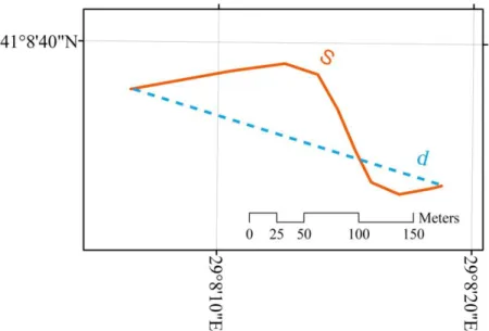
Spatial data has been used and produced rapidly in information age. This kind of production-consumption cycle brings several economic deficiencies because of duplicate versions of the same data. Geometric data integration relies on the combination of multi-source datasets to obtain up-to-date dataset without producing new data. This kind of integration is the subject of map conflation. Lynch and Saalfeld (1985) defined the purpose of map conflation that the objects in different datasets, representing the same entities, are combined to get a better map. Most of the conflation studies have been conducted on road networks because of the extensive usage such as navigation, transportation, etc. Main problem in conflation is matching road objects in different sources that represent the same road. Geo-object matching is a challenging study since there are several geometric, attribute and topological differences among source datasets. This is because of that the production of source datasets can be very different from each other in several ways such as coordinate system, date, data collection (on stereo image or surveying in field), and so on. It is a process that identifies, classifies and matches the object pairs, representing the same entity, with regards to their maximum similarity in whole datasets. The matching process is used to handle updating, aligning, optimizing, integrating, conflating and/or quality measuring of road networks. A matching algorithm is generally conducted by using similarity equations (Zhang and Meng, 2007; Li and Goodchild, 2011). The bigger similarity values the more possibility for matching candidates to be certain matched pairs. In similarity equations, there are several metrics (network alignment, distance threshold, orientation, direction, road length, valence, sinuosity, etc.) make the matching algorithm more efficient (Hacar and Gökgöz, 2016). While distance metric limits the number of matching candidates, orientation and valence (degree of connectivity) can be used to find the certain matches (Olteanu-Raimond et al., 2015; Mustière and Devogele, 2008). Sinuosity is also used to eliminate the incorrect candidates. It is a ratio of actual length of a road to the straight length among start and end points of the same road and defines how curve the road is (Mueller, 1968; Haynes et al., 2007) (Figure 1).
Figure 1. Actual (orange) and straight lengths (dashed blue) of a road
In this study, sinuosity intervals determined by commonly used classification methods and a proposed classification method called ‘sinuosity variance’ were compared with standard sinuosity intervals from Ireland Transportation Agency (ITA) under the framework of matching process. The study area and road datasets are described in Section 2. Besides, classification methods and proposed Sinuosity variance method are summarily introduced. In section 3, determination of sinuosity intervals were conducted and the results of matching process are presented with regards to the classification methods. Finally, some inferences from these results are given in section 4.
STUDY AREA AND DATASETS
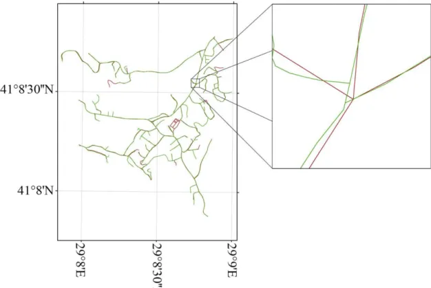
This study was conducted using datasets representing roads in Beykoz district, Istanbul, Turkey. It covers the area 1.6km x 1.7km. The road networks, representing the same entities, are one from Istanbul Metropolitan Municipality (IMM) road dataset and the other from Basarsoft navigation road dataset. Their pattern is tree-based. Figure 2 shows the study area, road networks and the differences among networks.
Figure 2. Study area and road datasets: IMM (green) and Basarsoft (red) Classification Methods
Roads are classified into predefined sinuosity intervals generally to analyze traffic components such as travel demand, road safety, etc. In the literature, there have been some calculations of sinuosity (Table 1).
Table 1. Some of the sinuosity measures (Haynes et al., 2007)
Method Definition
Bend density The number of bends per kilometer Sinuosity/detour
ratio
The ratio of actual length of a road to the straight length among start and end points of the same road
Straightness index The proportion of road segments that are straight
Mean angle The mean angle turned per bend In this study, the sinuosity/detour ratio is used as a sinuosity equation.
(1)
Sinuosity is commonly divided into three classes; Low → for straight and/or low curved roads Middle → for relatively curved roads
High → for highly curved roads.
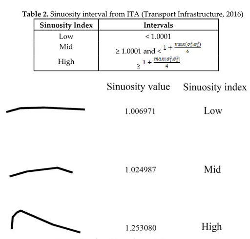
Sinuosity intervals (classes) can be determined by several commonly used data classification methods such as equal interval, quantile, natural breaks and geometrical interval. Furthermore, the intervals determined by ITA can be used in parallel with this purpose. ITA conducted an evaluation and defined three standardized sinuosity intervals for Ireland (Transport Infrastructure, 2016) (Table 2) (Figure 3).
Table 2. Sinuosity interval from ITA (Transport Infrastructure, 2016) Sinuosity Index Intervals
Low < 1.0001
Mid
≥ 1.0001 and < High
≥
Figure 3. Examples of road lines for each ITA sinuosity index.
In a matching process, the sinuosity index of an object is assumed to be the same sinuosity index of the matched object. For example, if Line A in dataset 1 has Low sinuosity index, then it is expected to search Low sinuosity indexed line/lines in dataset 2 during matching.
The proposed method sinuosity variance was also used to determine the intervals. In this method, sinuosity intervals were determined with regards to the variations of sinuosity values of the roads in datasets. Firstly, the sinuosity variance values in both road datasets are calculated. Then, the dataset has the maximum variance value is set to be a reference in order to calculate the sinuosity intervals (Table 3).
Table 3. Sinuosity interval calculations in sinuosity variance Sinuosity Index Intervals
Low < 1.0001 Mid
≥ 1.0001 and < High
≥
RESULTS AND DISCUSSION
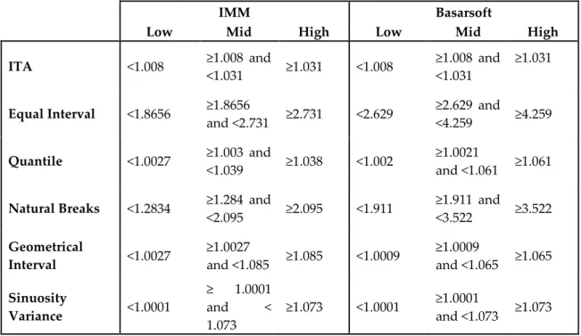
In this study, the sinuosity intervals were determined by using the proposed sinuosity variance approach, equal interval, quantile, natural breaks and geometrical interval. They were compared with standard intervals from ITA (Table 4 and 5).
Table 4. The sinuosity interval values retrieved from each classification method
IMM Basarsoft
Low Mid High Low Mid High
ITA <1.008 ≥1.008 and <1.031 ≥1.031 <1.008 ≥1.008 and <1.031 ≥1.031 Equal Interval <1.8656 ≥1.8656 and <2.731 ≥2.731 <2.629 ≥2.629 and <4.259 ≥4.259 Quantile <1.0027 ≥1.003 and <1.039 ≥1.038 <1.002 ≥1.0021 and <1.061 ≥1.061 Natural Breaks <1.2834 ≥1.284 and
<2.095 ≥2.095 <1.911 ≥1.911 and <3.522 ≥3.522 Geometrical Interval <1.0027 ≥1.0027 and <1.085 ≥1.085 <1.0009 ≥1.0009 and <1.065 ≥1.065 Sinuosity Variance <1.0001 ≥ 1.0001 and < 1.073 ≥1.073 <1.0001 ≥1.0001 and <1.073 ≥1.073
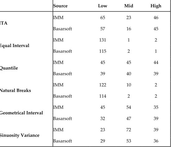
Table 5. Number of the objects in each sinuosity index with regards to the classification methods and sources
Source Low Mid High
ITA IMM 65 23 46 Basarsoft 57 16 45 Equal Interval IMM 131 1 2 Basarsoft 115 2 1 Quantile IMM 45 45 44 Basarsoft 39 40 39 Natural Breaks IMM 122 10 2 Basarsoft 114 2 2 Geometrical Interval IMM 45 54 35 Basarsoft 32 47 39 Sinuosity Variance IMM 23 72 39 Basarsoft 29 53 36
A pre-matching process was conducted by using Hausdorff distance with the threshold 85m. The threshold value should be determined as high as to catch all the possible candidate roads. The roads close to the others less than 85m were assigned to be matching candidates.
Line k and l are matched if the following conditions are met:
If Line k has ‘Low’ sinuosity index then Line l with ‘Low’ sinuosity index in all candidates of Line k is matched.
If Line k has ‘Mid’ sinuosity index then Line l with ‘Mid’ sinuosity index in all candidates of Line k is matched.
If Line k has ‘High’ sinuosity index then Line l with ‘High’ sinuosity index in all candidates of Line k is matched.
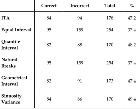
Matching processes were conducted after each classification. For the evaluation, the matching results were compared with manually matching results (Table 6).
Table 6. Matching statistics with regards to the classification methods. Correct Incorrect Total %
ITA 84 94 178 47.2 Equal Interval 95 159 254 37.4 Quantile Interval 82 88 170 48.2 Natural Breaks 95 159 254 37.4 Geometrical Interval 82 91 173 47.4 Sinuosity Variance 84 86 170 49.4 CONCLUSIONS
In this study, a new method determining sinuosity intervals and classifying sinuosity index for road matching process was proposed. Sinuosity intervals were determined with regards to the variations of sinuosity values of the roads in datasets. It is compared with the sinuosity intervals from ITA and mostly used classification methods. Equal Interval and Natural Breaks methods are insufficient for matching process since hardly any roads were classified into ‘Mid’ or ‘High’ sinuosity indices. Quantile method gave the second best result. In this method, the intervals are determined to make each sinuosity class has the same number of objects. Since both datasets in this study have different number of objects, Quantile should be tested better with datasets that have the same number of objects. Sinuosity variance, a promising classification method for matching process, gave the best matching result in all classification methods.
ACKNOWLEDGEMENT
Authors would like to thank Istanbul Metropolitan Municipality Directorate of Geographical Information Systems, and Basarsoft Information Technologies Inc. for supplying road data.
REFERENCES
Hacar, M., Gökgöz, T., 2016, “An Experiment on Distance Metrics used for Road Matching in Data Integration”, Sigma Journal of Engineering and Natural Sciences, Vol. 34(4), pp. 527-542.
Haynes, R., Jones, A., Kennedy, V., Harvey, I., Jewell, T., 2007, “District Variations in Road Curvature in England and Wales and Their Association with Road-Traffic Crashes” Environment and Planning A, Vol. 39(5), pp. 1222-1237.
Li, L., Goodchild, M.F., 2011, “An Optimisation Model for Linear Feature Matching in Geographical Data Conflation”, International Journal of Image and Data Fusion, Vol. 2(4), pp. 309-328.
Lynch, M. P., Saalfeld, A. J., 1985, “Conflation: Automated Map Compilation—A Video Game Approach”, In Proceedings Auto-Carto, Vol. 7, pp. 343-352.
Mueller, J. E., 1968, “An Introduction to the Hydraulic and Topographic Sinuosity Indexes” 1. Annals of the Association of American Geographers, Vol. 58(2), pp. 371-385.
Mustière, S., Devogele, T., 2008, “Matching Networks With Different Levels of Detail”, GeoInformatica, Vol. 12(4), pp. 435-453.
Olteanu-Raimond, A. M., Mustiere, S., Ruas, A., 2015, “Knowledge Formalization for Vector Data Matching Using Belief Theory”, Journal of Spatial Information Science, Vol. 2015(10), pp. 21-46. Transport Infrastructure, 2016, National Road Network Sinuosity Index: Ireland,
https://data.gov.ie/dataset/national-road-network-sinuosity-index (Accessed on 1 September 2018). Zhang, M., Meng, L., 2007, “An Iterative Road-Matching Approach for the Integration of Postal Data”,